WindPRO Tips & Tricks

WindPRO Tips & Tricks
Elevation Grid Data as alternative to Line Object Data.
The elevation grid object as a new object in V2.8 offers a number of benefits – and perhaps
also some “slightly hidden” features, which you might not have discovered yet. Below we have
highlighted some of the advantages of this new object:
• Ideal for importing gridded data (SRTM, xyz files etc.) - Data remain in the
“original format”.
• Handles more layers - Data in calculations are always taken from upper layer first (if
data exist). Thus, large areas can be covered with a high resolution in the most
important areas and less at distance. This means that the user can work with a high
accuracy without the risk of running out of memory!
• Import huge data amounts - Data from e.g. a laser scanning survey (which might be
irregular gridded) can be imported with data reduction and converted to regular gridded
data. This means that the often huge data amount can be handled very efficiently.
• Create an editable layer – Data from a specified subarea are simply exported to a
line object, (contour data) with all the “normal” edit features, and after editing it is
automatically feed back into the elevation grid object. This way the important areas
e.g. near a measurement mast are handled very precise in the WAsP calculations.
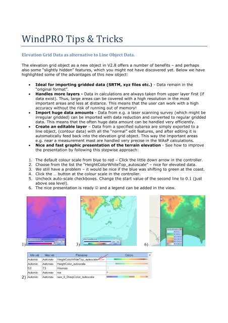
• Nice and fast graphic presentation of the terrain elevation - See how to improve
the presentation by following this stepwise approach:
1. The default colour scale from blue to red – Click the little down arrow in the controller.
2. Choose from the list the “HeightColorWhiteTop_autoscale” – nice for elevated data.
3. We still have a problem – it would be nice if the blue was shifting to green at the coast.
4. Click the … button at the colour scale in the controller.
5. Uncheck auto-scale checkboxes. Change the start value of the second line to 0.1 (just
above sea level).
6. The nice presentation is ready ☺ and a legend can be added in the view.
1) 3) 6)
2)

4)
5)
Use Google Earth to place Noise Sensitive Areas(Points) (NSA’s).
With the Google Earth synchronization it is very easy to place Noise Sensitive Points (NSA’s)
precisely on the map (or other objects, e.g. control points for photo calibration).
Open the embedded Google map window and insert an NSA on the approximate position
of the dwelling on the map. You will now see the object appear on the Google Earth window.
Drag the object on the map until it is located on the most exposed point of the dwelling.
HINT: You can fine adjust position by selecting the object (single left mouse click), then hold
down and use arrows.
Some noise codes require the NSA to be located a certain distance from the dwelling. In e.g.
Denmark two sets of NSA’s are required, one for “normal noise”, at nearest outdoor occupation
area at the property, max. 15 m from the dwelling in direction of the turbines, and one for Low
Frequency(LF) noise, located at the dwelling. To establish such two sets:
Create two object layers, one for most exposed points of the dwellings (for LF noise), and
another for NSA’s at a fixed distance from the dwelling (for normal noise).
For the layer with LF objects, show distance circle at radius 15 m (right click menu on
layer):

Now create NSA for LF in this layer.
Then create the NSA for “normal noise” in the other layer –place it on the distance circle in
direction of the turbines.
You can immediately see on the Google Earth window if the “normal noise” NSA point is
correctly placed within the property of the dwelling.