The Canonical Distribution of Commonness and Rarity: Part I F. W ...

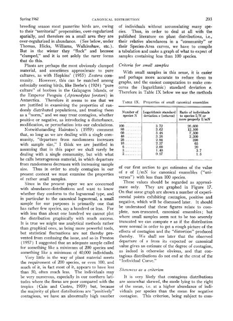
Spring 1962
CANONICAL DISTRIBUTION
breeding season most passerine birds are, o~vi~lg of individuals without accumulating many speto
their "territorial" propensities, over-regularized
spatially, and therefore on a small area they are
over-rqgularized in abundance. (See below, under
Thomas, Hicks, Williams, I'dalkinshaw, etc.) .
cies. Thus, in order to deal at all with the
But in the winter they "flock" and become
"clumped," and it is not solely the rarer forms
that do this.
Plants are perhaps the most obviously clumped
material, and sometimes approximate to pure
cultures, as with Hopkins' (1955) Zostera community.
However, this can be matched among
colonially nesting birds, like Beebe's ( 1924) "pure
culture" of boobies in the Galapagos Islands. or
the Emperor Penguin (Apfertodytes forsteri) in
Antarctica. Therefore it seems to me that we
are justified in examining the properties of randomly
distributed populations, and treating them
as a "norm," and we nlay treat contagion, whether
positive or negative, as introducing a disturbance,
modification, or perturbation into our calculations.
Notwithstanding Hairston's ( 1959) comment
that, so long as vie are dealing with a single community,
"departure from randomness increases
with sample size," I thillk we are justified in
assuming that in this paper we shall rarely be
dealing .n-it11 a single community, but with what
he calls heterogenous material, in which departure
fro111 randomness decreases with increasing saniple
size. Thus in order to study contagion in our
present context we must examine the properties
of rather small samples.
Since in the present paper we are concerned
with abundance-distributions and want to know
whether they conforn~ to the lognormal type, and
in particular to the canonical lognormal, a small
sample for our purposes is primarily one that
has rather few species, say a hundred or less. For
with less than about one hundred we cannot plot
the distribution graphically with much success.
It is true we might use analytical methods rather
than graphical ones, as being more powerful tools,
but statistical fluctuations are not thereby prevented
from confusing the issue, and so in Preston
(1957) I suggested that an adequate sample called
for something like a minimum of 200 species and
something like a mitlimum of 30,000 individuals.
Very little in the way of plant material meets
the requirement of 200 species. or eveti 100. and
much of it, in fact most of it, appears to have less
than 50, often much less. The individuals may
be very numerous, especially in our northern latitudes
where the floras are poor compared with the
tropics (Cain and Castro, 1959) but, because
the majority of plant distributions are "positively"
contagious, we have an abnormally high ntltnber
203
published literature on plant distributions, i.e.,
their relative abundances in a "community" or
their Species-Area curves, we have to compile
a tabulation and make a graph of what to expect of
samples containing less than 100 species.
Criteria for s~~lall sar?tples
With small samples in this sense, it is easier
and perhaps more accurate to reduce them to
graphs, and the easiest computation to make concerns
the (logarithmicj standard deviation o.
Therefore in Table I9 below we use the methods
TABLEIX. Properties of small canonical ensembles
I
I
Number of Logarithmic standard Ratio of individuals
species S deviation a (octaves) to species I/N or
more properly I/mN
of our first section to get estimates of the value
of 5 of 1,'mK ior canonical ensembles ("universes")
with less than 100 species.
These values shorrld be regarded as approximate
only. They are graphed in Figure 17.
On that same graph are shown a number of experimental
points exhibiting contagion, positive and
negative, which will he discussed later. It should
be understood that these figures relate to cornplete,
non-truncated, canonical ensembles; but
where small samples seem not to be too severely
truncated we can compute o as if the distribution
were normal in order to get a rough picture of the
effects of coritagion and the "distortion" produced
thereby. 11-e shall see later that the observed
departure of s from its expected or canonical
value gives an estimate of the degree of contagion,
as indeed is otherwise obvious, and that contagious
distributions do not end at the crest of the
"Individual Curve."
Skcrcwess us n criterion
It is very likely that contagious distributions
are soniewhat skewed, the mode lying to the right
of the mean, i.e. at a higher abundance of individuals
per species than the mean for negative
contagion. This criterion, being subject to com-