The Canonical Distribution of Commonness and Rarity: Part I F. W ...
The Canonical Distribution of Commonness and Rarity: Part I F. W ...
The Canonical Distribution of Commonness and Rarity: Part I F. W ...

Create successful ePaper yourself
Turn your PDF publications into a flip-book with our unique Google optimized e-Paper software.
Spring 1962<br />
CANONICAL DISTRIBUTION<br />
211<br />
FIG.25. A family <strong>of</strong> generalized parabolas, <strong>and</strong> the<br />
locus <strong>of</strong> points <strong>of</strong> maximum curIrature.<br />
point <strong>of</strong> sharpest curvature. In this sense there<br />
is a theoretical "break" in the curve, though it<br />
is not a discontinuity <strong>of</strong> any sort.<br />
<strong>The</strong> curvature <strong>of</strong> any curve at any point is<br />
given by<br />
<strong>and</strong> if we differentiate this once more <strong>and</strong> set<br />
<strong>and</strong> solve for x, we can define the point <strong>of</strong> maximum<br />
curvature in terms <strong>of</strong> the abscissa, or by<br />
solving for y we can define it in terms <strong>of</strong> the<br />
ordinate. which is usually (in our problem) more<br />
satisfactory.<br />
In this case, we find that the point is given by<br />
On Fig. 25 I have plotted the locus <strong>of</strong> the maximum<br />
curvature. It is probably the break-point<br />
that Cain was seeking. In practice, however, it<br />
is not easy to determine such a point by graphical<br />
methods. It is much easier, even with a curve<br />
perfectly free from experimental or statistical<br />
errors, to find the point by equation (32), <strong>and</strong> for<br />
that purpose we have first to find the value <strong>of</strong> n.<br />
Clearly, if the curve really is a parabola, this is<br />
most easily done by taking logarithms <strong>of</strong> both<br />
ordinate <strong>and</strong> abscissa, whereon the equation becomes<br />
11 log y = log a + log x (33)<br />
which is a linear relation between log (Species)<br />
<strong>and</strong> log (Area) : i.e. the curve ought to be a<br />
straight line. This log-log plotting I have elsewhere<br />
(' Preston 1960) called an Arrhenius plot-<br />
' I am indebted to Dr. R. E. mould <strong>of</strong> Preston Laboratories,<br />
Inc., no\v Xtnerican Glass Research, Itlc., for this<br />
result,<br />
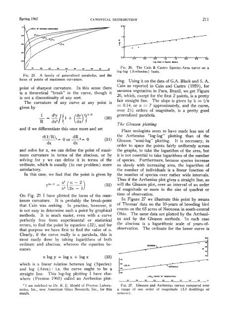
FIG.26. <strong>The</strong> Cain & Castro Species-Area curve on a<br />
log-log (Arrhenius) basis.<br />
ting. Using it on the data <strong>of</strong> G.A. Black <strong>and</strong> S. A.<br />
Cain as reported in Cain <strong>and</strong> Castro (1959)) for<br />
savanna vegetation in Para, Brazil, we get Figure<br />
26, which, except for the first 2 points, is a pretty<br />
fair straight line. <strong>The</strong> slope is given by k = l/n<br />
= 0.14, or n = 7 approximately, <strong>and</strong> the curve,<br />
over 225 orders <strong>of</strong> magnitude, is a pretty good<br />
generalized parabola.<br />
<strong>The</strong> Gleas<strong>of</strong>i plotting<br />
Plant ecologists seem to have made less use <strong>of</strong><br />
the Arrhenius "log-log" plotting than <strong>of</strong> the<br />
Gleason "semi-log" plotting. It is necessary, in<br />
order to space the points fairly uniformly across<br />
the graphs, to take the logarithm <strong>of</strong> the area, but<br />
it is not essential to take logarithms <strong>of</strong> the number<br />
<strong>of</strong> species. Furthermore, because species increase<br />
so slowly with increasing area, the logarithm <strong>of</strong><br />
the number <strong>of</strong> individuals is a linear function <strong>of</strong><br />
the number <strong>of</strong> species over rather wide intervals.<br />
Thus if the Arrhenius plot gives a straight line, so<br />
will the Gleason plot, over an interval <strong>of</strong> an order<br />
<strong>of</strong> magnitude or more in the size <strong>of</strong> quadrat or<br />
time <strong>of</strong> observation.<br />
In Figure 27 we illustrate this point by means<br />
<strong>of</strong> Thomas' data on the 10-years <strong>of</strong> breeding bird<br />
counts on the 65 acres <strong>of</strong> Neotoma in south-central<br />
Ohio. <strong>The</strong> same data are plotted by the Arrhenius<br />
<strong>and</strong> by the Gleason methods. In each case<br />
the abscissa is a logarithmic scale <strong>of</strong> years-<strong>of</strong>observation.<br />
<strong>The</strong> ordinate for the lower curve is<br />
FIG.27. Gleason <strong>and</strong> Arrhenius curves compared over<br />
a range <strong>of</strong> one order <strong>of</strong> magnitude (3.3 doublings or<br />
octaves).