The Canonical Distribution of Commonness and Rarity: Part I F. W ...
The Canonical Distribution of Commonness and Rarity: Part I F. W ...
The Canonical Distribution of Commonness and Rarity: Part I F. W ...

Create successful ePaper yourself
Turn your PDF publications into a flip-book with our unique Google optimized e-Paper software.
<strong>The</strong> <strong>Canonical</strong> <strong>Distribution</strong> <strong>of</strong> <strong>Commonness</strong> <strong>and</strong> <strong>Rarity</strong>: <strong>Part</strong> I<br />
F. W. Preston<br />
Ecology, Vol. 43, No. 2. (Apr., 1962), pp. 185-215.<br />
Stable URL:<br />
http://links.jstor.org/sici?sici=0012-9658%28196204%2943%3A2%3C185%3ATCDOCA%3E2.0.CO%3B2-8<br />
Ecology is currently published by Ecological Society <strong>of</strong> America.<br />
Your use <strong>of</strong> the JSTOR archive indicates your acceptance <strong>of</strong> JSTOR's Terms <strong>and</strong> Conditions <strong>of</strong> Use, available at<br />
http://www.jstor.org/about/terms.html. JSTOR's Terms <strong>and</strong> Conditions <strong>of</strong> Use provides, in part, that unless you have obtained<br />
prior permission, you may not download an entire issue <strong>of</strong> a journal or multiple copies <strong>of</strong> articles, <strong>and</strong> you may use content in<br />
the JSTOR archive only for your personal, non-commercial use.<br />
Please contact the publisher regarding any further use <strong>of</strong> this work. Publisher contact information may be obtained at<br />
http://www.jstor.org/journals/esa.html.<br />
Each copy <strong>of</strong> any part <strong>of</strong> a JSTOR transmission must contain the same copyright notice that appears on the screen or printed<br />
page <strong>of</strong> such transmission.<br />
<strong>The</strong> JSTOR Archive is a trusted digital repository providing for long-term preservation <strong>and</strong> access to leading academic<br />
journals <strong>and</strong> scholarly literature from around the world. <strong>The</strong> Archive is supported by libraries, scholarly societies, publishers,<br />
<strong>and</strong> foundations. It is an initiative <strong>of</strong> JSTOR, a not-for-pr<strong>of</strong>it organization with a mission to help the scholarly community take<br />
advantage <strong>of</strong> advances in technology. For more information regarding JSTOR, please contact support@jstor.org.<br />
http://www.jstor.org<br />
Sat Dec 1 08:27:18 2007
ECOLOGY <br />
iro~. 43 SPRIKG 1962 No. 2<br />
THE CXNONICPlL DISTRIBUTION OF COMhiONNESS AND RARITY: PART I<br />
F. Ji. PRESTOS<br />
Prc sfoli Lal~oriifi~rlis, Blrtlrr. Prrirts~ l~~riiio<br />
In an earlier paper ( Preston 1948 ) we found<br />
that, in a sufficiently large aggregation <strong>of</strong> individuals<br />
<strong>of</strong> many species, the individuals <strong>of</strong>ten<br />
tended to be distributed among the 5pecies according<br />
to a lognormal law. We plotted as abscissa<br />
equal increments in the logarithms <strong>of</strong> the number<br />
<strong>of</strong> individuals representing a species, <strong>and</strong> as orclinate<br />
the number <strong>of</strong> species falling into each <strong>of</strong><br />
these increments. We found it collvenient to use<br />
as such increments the "octave," that is the interval<br />
in which representation donbled, so that<br />
our abscissae became simply a scale <strong>of</strong> "octaves,"<br />
but this choice <strong>of</strong> unit is arbitrary. IVhatever<br />
logarithmic unit is used, the graph tended to talie<br />
the form ot a iiornlal or Gaussian curve, so that<br />
the d~str~bution was "logi~orn~al." 11-e called this<br />
the "Sprcies Curve."<br />
In the present paper we take up a point nierely<br />
nientioiied in 194s that not only is the distribution<br />
log~~ormal. but the constants or parameters seein<br />
to he restricted in a peculiar way. <strong>The</strong>y are not<br />
fixed, but they are interlocked. <strong>The</strong> nature <strong>of</strong><br />
this restriction <strong>and</strong> iriterlocking 1s the main theme<br />
<strong>of</strong> the present paper.<br />
I11 the earlier paper we graduated the experimental<br />
results with curves <strong>of</strong> the form<br />
= e-':'~"<br />
0<br />
(1)<br />
where y is the number <strong>of</strong> species falling into the<br />
Rth "octave" to the right or left <strong>of</strong> the mode, yo<br />
is the number in the modal octave, <strong>and</strong> a was<br />
treated as an arbitrary constant, to be found from<br />
the experimental evidence. This constant is related<br />
to the logarithmic st<strong>and</strong>ard deviation a by<br />
the formula<br />
a2 = Ma2 (2)<br />
<strong>and</strong> we noted that it had a pronoutlced tendency<br />
to come out at a figure not far from 0.2, so that a<br />
would have a value <strong>of</strong> about 3.5 octaves, <strong>and</strong>, since<br />
there are 3.3 octaves to an "order <strong>of</strong> magnitude,"<br />
a would be a little more than an order <strong>of</strong> magnitude.<br />
If we now make a 2nd graph in which, using<br />
the same abscissae, we plot as ordinate not the<br />
number <strong>of</strong> species (y) that fall in each interval<br />
but the nunlber <strong>of</strong> individuals which those y species<br />
comprise, we get another lognormal cnrve<br />
with the same st<strong>and</strong>ard deviation as the first<br />
graph, but with its mode or peak displaced to the<br />
right. This we call the "Individuals Curve."<br />
Though we can use a Gaussian curve to "graduate"<br />
the observed points <strong>of</strong> the species curve, the<br />
curve extends infinitely far to left <strong>and</strong> right, while<br />
the number <strong>of</strong> observed points is necessarily finite.<br />
This is a common situation in statistical worlc <strong>and</strong><br />
usuallj causes no complications, hut in our problem<br />
there results an additional piece <strong>of</strong> information.<br />
<strong>The</strong> Individuals Curve ~iecessarily lacks at<br />
least part <strong>of</strong> the descending limb. It terminates<br />
over the last observed point <strong>of</strong> the Species Curve,<br />
<strong>and</strong> this is long before the Individuals Curve begins<br />
to l~ecorne asymptotic to the horizontal axis.<br />
111 the earlier paper we noted that, as a matter <strong>of</strong><br />
obser~.ation,it seenls to terminate at its crest, so<br />
that, in effect, only half <strong>of</strong> the curve is present.<br />
\Yhat I failed to observe in 1938 was that when<br />
the Individuals Curve terminates at its crest or<br />
very close to it, the value <strong>of</strong> "a" in equation (1)<br />
<strong>and</strong> <strong>of</strong> the st<strong>and</strong>ard deviation "a," is fixed within<br />
narrow limits, <strong>and</strong> this value is in fact the one<br />
actually observed. This does not mean that "a"<br />
is a true constant, but only that it is not iudependent<br />
<strong>of</strong> y, or <strong>of</strong> the total number <strong>of</strong> species, N.<br />
It may be said that "a" is a function <strong>of</strong> yo, so that<br />
given one, the other is settled. Thus we are reduced<br />
from 2 seemingly disposable parameters or<br />
constants to one. More generally, given any<br />
one piece <strong>of</strong> information about our collection, for<br />
instance given either the total number <strong>of</strong> species
186 FRANK W. PRESTON Ecology, Val. 43, No. 2<br />
or the total number <strong>of</strong> individuals, everything else<br />
is fixed.<br />
<strong>The</strong> zuord "<strong>Canonical</strong>"<br />
I have ventured to call such an equation<br />
"canonical." It appears likely that this term was<br />
introduced into mathematical physics by J. Willard<br />
Gibbs: I quote from the preface to I'olume<br />
2 <strong>of</strong> his Collected \I-orks 1 1931) : "11-e return to<br />
the consideration <strong>of</strong> statistical ecluilibriunl . . .<br />
we consider especially ensembles <strong>of</strong> systems in<br />
which the logarithm <strong>of</strong> probability <strong>of</strong> phase is a<br />
linear function <strong>of</strong> the energy. This distribution,<br />
on account <strong>of</strong> its unique importance in the theory<br />
<strong>of</strong> statistical equilibrium, I have ventured to call<br />
canonical" (italics his).<br />
L3y a sort <strong>of</strong> rough analogy, I have designated<br />
as "canoilical," for ecological purposes, that particular<br />
lognorn~al distribution <strong>of</strong> the abundatlces<br />
<strong>of</strong> the various species (or genera. families, etc.)<br />
whose "Individuals Curve" terminates at its crest.<br />
This way <strong>of</strong> describing it is probably imperfect,<br />
<strong>and</strong>, as shown later, it apparently corresponds to<br />
a situation in space or time where the individuals,<br />
or pairs, are distributed at r<strong>and</strong>om, not clumped<br />
on the one h<strong>and</strong> nor over-regularired on the<br />
other. Thus a better definition may be possible,<br />
<strong>and</strong> in that case preferable; but, however defined,<br />
it is a distribution that seems to ha\-e special importance<br />
in the general theory <strong>of</strong> ecological ensembles,<br />
<strong>and</strong> so I have ventured to call it "canonical."<br />
In the present paper we trace the consequeilces<br />
<strong>of</strong> assuming the distribution canonical. \Ve examine<br />
how nearly the experimental res~~lts fit the<br />
purely theoretical curves. <strong>The</strong>se experimeiltal results,<br />
though sonie <strong>of</strong> then1 involve "collections"<br />
having many millions <strong>of</strong> individuals, take us only<br />
as far as a few hundred species. \Ye attempt<br />
to estimate what would happen if we had<br />
thous<strong>and</strong>s or scores <strong>of</strong> thous<strong>and</strong>s <strong>of</strong> species, where<br />
we have no actual counts <strong>of</strong> individuals but may<br />
sometimes be able to estimate them roughly, <strong>and</strong><br />
we draw such other tentative conclusions as occur<br />
to us.<br />
As the scale <strong>of</strong> abscissae we may use octaves,<br />
which is equivalent to taking "logarithms to the<br />
base 2," as we did in 1948, or we may use "orders<br />
<strong>of</strong> magnitude" ~vhich is more conveilient when<br />
dealing with very large numbers. This is equivalent<br />
to taking logarithms to hase 10 as James<br />
Fisher ( 1952) did. For theoretical purposes a<br />
scale <strong>of</strong> natural logarithms (i.e to hase 2.718)<br />
would be most convenient. IYilliams (1953)<br />
iound it convenient to work with logarithms to<br />
base 3.<br />
Cotiseq~ietices <strong>of</strong> assuming that the individuals<br />
curve terminates at its crest<br />
This matter may be stated briefly, anticipating<br />
the more detailed statement <strong>of</strong> the next heading,<br />
as follours: As shown in Preston (1948) the<br />
distance between the crests <strong>of</strong> the Species <strong>and</strong><br />
Individuals Curves is In 2/(2a2) or (In 2)u2,<br />
where o is the logarithmic st<strong>and</strong>ard deviation in<br />
octaves.<br />
Though we describe our distribution as lognormal,<br />
it actually is finite, <strong>and</strong> species <strong>and</strong> individuals<br />
are not found infinitely distant from the<br />
mode either to the right or the left. In industrial<br />
"quality control" work it is customary to say that<br />
not more than one specimen out <strong>of</strong> a thous<strong>and</strong><br />
should be expected beyond the 3-sigma limit, but<br />
in none <strong>of</strong> the biological examples me have yet<br />
encountered do we have as many as a thous<strong>and</strong><br />
species to work with. \Ire should therefore expect<br />
the finite distribution to end short <strong>of</strong> the 3-sigma<br />
limit. In fact, wit11 the number <strong>of</strong> species in our<br />
examples to date we should expect it to terminate<br />
at about 2.5 to 2.8 sigma. If we take the latter<br />
zalue, the assumption that the distributions terminate<br />
where the Individuals Curve reaches its crest<br />
is erluivalent to setting<br />
(111 2)02 = 2.&, or 5 = 4.0 octaves approximately.<br />
But this is just about what we find in our observations;<br />
it correspoi~ds to an "a" value <strong>of</strong><br />
0.175.<br />
Thus by an appeal to observation, but not by<br />
pure theory, we can reach the conclusion that<br />
very <strong>of</strong>ten the finite distribution does in fact end<br />
just about where the Individuals Curve reaches<br />
its crest. This seems to make it advisable to<br />
restate the matter more formally, in order to cover<br />
the complete range <strong>of</strong> possible values <strong>of</strong> the<br />
number <strong>of</strong> species involved.<br />
Tll c I~tdividl(a1s Curve<br />
In the Specles Curve each octave contains a<br />
certain tiumber <strong>of</strong> species <strong>and</strong> each <strong>of</strong> these is<br />
represented hy roughly the same nun~ber <strong>of</strong><br />
individuals. hlultiplying the one figure by the<br />
other gives the total number <strong>of</strong> individuals that<br />
have, in effect, been assigned to that octave. By<br />
making this computation for each octave we can<br />
construct the "Individuals Curve." This can be<br />
done for the observed points, but here we are<br />
concerned with its theoretical form.<br />
For the Species Curve we haxe, as in equation<br />
(1) above<br />
= ?-a?~?<br />
0 0<br />
Let the number <strong>of</strong> individuals per species, the
Spring 1962<br />
CANONICAL<br />
"representation" <strong>of</strong> the species, be no at the modal<br />
octave. <strong>The</strong>n at the Rth octave from the mode it<br />
is n,ZR individuals per species, <strong>and</strong> the octave<br />
holds yn,2R individuals, or :<br />
Y = (noyo)[2Re-aeRS]= (noyo)[eRIn e-a2~2]<br />
- noyo (IL&) \-&2(RR~2) 2<br />
2a 2a2 (3)<br />
This is a lognormal curve with the mode dis-<br />
In 2<br />
placed by an amount - octaves : it has the same<br />
2a2<br />
dispersion constant as the Species Curve, <strong>and</strong> it<br />
has the modal height Yo= noyoe(s)2.<br />
(See Figure 1.)<br />
Equations like (3) become somewhat simpler<br />
in appearance if ive use "natural orders <strong>of</strong> magnitude"<br />
in place <strong>of</strong> "octaves," i.e. if we use intervals<br />
in which the frequency or abundance <strong>of</strong> a<br />
species increases in the ratio 2.718 instead <strong>of</strong> 2.0,<br />
<strong>and</strong> if we use F, the st<strong>and</strong>ard deviation in orders<br />
<strong>of</strong> magnitude, instead <strong>of</strong> the coefficient a.<br />
This method <strong>of</strong> working is convenient if we<br />
have available adequate tables <strong>of</strong> natural logarithms,<br />
for then the observed frequencies are easily<br />
DISTRIBUTION 187<br />
classified into their natural orders <strong>of</strong> magnitude.<br />
I think, however, that it will be more convenient<br />
if we continue, as we have begun, by using "octaves,"<br />
which do not depend on the availabilitv<br />
<strong>of</strong> such tables, or on thk alternative method df<br />
cotlverting ordinary logarithms to natural ones.<br />
<strong>The</strong> eflects <strong>of</strong> a finite number <strong>of</strong> species<br />
Referring to the Species Curve in Figure 1, we<br />
note that in theory this curve extends infinitely<br />
far both to left <strong>and</strong> to right, but the long "tails"<br />
are exceedingly close to the R axis as asymptote.<br />
<strong>The</strong> area under the cunre, or the integral <strong>of</strong> the<br />
curve, represents the number <strong>of</strong> species we have<br />
accumulated, as we go from minus infinity to any<br />
given point. This area is at first so small that<br />
not until we are within about 9 octaves <strong>of</strong> the<br />
mode (for this particular case, where we have<br />
a total <strong>of</strong> 178 species) have we accumulated<br />
enough area to correspond to a single species.<br />
This is the beginning <strong>of</strong> the real, finite, distribution.<br />
As we continue to the right we accumulate<br />
species rapidly; then we pass the mode <strong>and</strong><br />
accumulate them increasingly slowly. Finally<br />
we reach a point some 9 octaves to the right <strong>of</strong><br />
the mode where the remaining area is scarcely<br />
enough to hold one more species. In practice,<br />
/+-<br />
lntermodal Distance <br />
2)ILaz .-I<br />
1<br />
) SCALE OF OCTAVES<br />
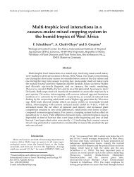
FIG.1. <strong>The</strong> canonical distribution ior an ensemble <strong>of</strong> 178 species. For this number oi species, the coefficient<br />
a = 0.200 <strong>and</strong> the st<strong>and</strong>ard deviation o is 3.53 octaves for both "Species" <strong>and</strong> "Individuals" curves. <strong>The</strong> modal<br />
height <strong>of</strong> the species curve is y, = X, species. <strong>The</strong> ordinate scale for the individuals curve is arbitrary: see text<br />
for explanation. <strong>The</strong> intermodal distance is 8.68 octaves. <strong>The</strong> real part <strong>of</strong> each curve is drawn solid : the first<br />
(rarest) <strong>and</strong> last (comtnonest) species ought to lie at about this distance (8.68 octaves or 2.45 a) from the<br />
mode <strong>of</strong> the species curve, or perhaps a little, but only a little, more.
188 FRANK W. PRESTON Ecology. Val. 43. Xo 2<br />
the finite distribution ends at, or near, this point.<br />
<strong>The</strong> nutnerical value <strong>of</strong> the integral between<br />
any specified limits can be found from published<br />
tables, but the integral itself cannot be expressed<br />
readily in analytical form, suitable for finding a<br />
general solution to our problems. Nor, if it<br />
could, would it define the end <strong>of</strong> the clistribution<br />
with real precision; at best it can only give an<br />
idea <strong>of</strong> the most probable position <strong>of</strong> the end <strong>of</strong><br />
the distribution. 1Ye have taken as the most<br />
prolxible position that pint lvhere the remaining<br />
area under the tail <strong>of</strong> the curve corresponds to<br />
half a species. This mean that there is a 1 :1<br />
chance that we have not quite reached the end or<br />
that we have just passed it.<br />
In Tahle I we have given, for various values <strong>of</strong><br />
TABLEI. <strong>The</strong> parameters <strong>of</strong> the canollical ensemble<br />
K r s a y o R~.. r 12 l/m<br />
100... 2.576 3 .i2 0.190 10.7 9.58 765 5.8XlOj ?.69X10"<br />
200.. 2.807 4.05 0.175 19.7 11.4 2,i20 7.40X10⁶ 3.i5X10'<br />
400.. . 3.024 4.36 0.16? 36.6 13.2 9,410 8.85X10' 4.82XlOS<br />
SO0... 3.227 4.66 0.152 68.5 15.0 32,iiO 1.0iX10~6.23XlOQ<br />
1,000 .. 3.291 4.i5 0.149 84.0 15.6 49,6iO?.4iX109 l.4iX10lL'<br />
3,000 . . 3.481 5.02 0.141 158.9 li.5 lS5,iOO 3.44XlOlo ?.16XlOl1<br />
4,000.. . 3.662 5.28'0 134 302 19.3 645.500 4.liXlOll ?..i5X101?<br />
8,000,. 3.836 5.5110:12S 57621.2 2,409,000 5.8OXl0~2I.r)%XlO'"<br />
?l.8 3,631,00011.33~10~~<br />
10,000 .. 3.891 5.61 0.126 ill 0.93~10"<br />
100,000 . 4.418 5.38 0.111 6,130 28.2 L68XlOs 8.29~10'66.61XlO1;<br />
1,000,000 .. 4.892 7.060.100 56,500 31.5 ,2.43~10~o5.90~10~o 5.21X10²¹<br />
(Note.<br />
In 2 = 0.89315 <strong>and</strong> thereciprocal<strong>of</strong> thisis 1.143'1cis to beascertained<br />
by multiplying x by 1.443.<br />
<strong>The</strong>n a is to be ascertained by dividing O.iO7 by a.<br />
<strong>The</strong>n yo is to be ascertained from the formula yo = 0.3989 N/a.<br />
RmSlI! to be ascertained by multiplying x by 5.<br />
the total number, K, <strong>of</strong> species involvedj that<br />
value <strong>of</strong> x, or R,,,,/'cr,' which makes<br />
That is to say, we have left one species out <strong>of</strong> K<br />
to be divided between the two tails, to left <strong>of</strong> -s<br />
<strong>and</strong> to right <strong>of</strong> +x, or half a species per tail. <strong>The</strong><br />
values are taken from Lowan (1912).<br />
It can be shown that this point is very nearly<br />
the same as would be obtained by setting y = 0.4<br />
(species per octave ) in equation ( 1j , which would<br />
give<br />
JVe now have to trace the consecluences <strong>of</strong><br />
assuming that the crest <strong>of</strong> the Individuals Curve<br />
coincides with the finite end <strong>of</strong> the Species Curve.<br />
Estivzating the cano,zical co~lstaltts<br />
TVe have seen that the distance between the<br />
' Note that this defines x as the half-range in terms <strong>of</strong><br />
the logarithmic st<strong>and</strong>ard deviation, T, as the unit.<br />
n~odes <strong>of</strong> the species <strong>and</strong> individuals curves is<br />
ln2)/2a2 = a2 11-12, <strong>and</strong> from Table I we have<br />
the values <strong>of</strong> Rmar/u or "x." Equating the two<br />
we have<br />
whence<br />
Since n7e already have the values <strong>of</strong> x for various<br />
values <strong>of</strong> N?the total number <strong>of</strong> species, we are<br />
now i11 a position to add to Table I the values <strong>of</strong><br />
3 <strong>and</strong> <strong>of</strong> R,,,: <strong>and</strong> this has been done. Further,<br />
since a% 1/25' or a = O.49/x, we can also add<br />
the value <strong>of</strong> a. Again, the number <strong>of</strong> species<br />
(yd in the ~noclal octave <strong>of</strong> the Species Curve can<br />
also be computed, for<br />
-<br />
r\; = s., ~ t ' 2 ~<br />
so that<br />
yo = 0.399 K o = 0.277 iY 'x. ' 8)<br />
This value, also, is therefore added to Table I<br />
<strong>and</strong> this completes all the unknowns. Given the<br />
total numlxr <strong>of</strong> species, the first column <strong>of</strong> Table<br />
I, we can ascertain all the coiista~lts <strong>of</strong> equation<br />
(1 I. <strong>The</strong> basic equation <strong>of</strong> the distribution has<br />
therefore become canonical, in the sense that<br />
nothing is left to chance: once X is specified,<br />
everj.thing is determined.<br />
Tlle relatiotj brtu'een total i~zdizidilals <strong>and</strong><br />
total sp~cies<br />
<strong>The</strong> canonical equation implies that there is a<br />
definite relationship between these 2 quantities,<br />
<strong>and</strong> if "In," as defined below, is known, it is easily<br />
calculated. 11-hen we permit ourselves the liberty<br />
ot' making this theoretical estimate, me can expect<br />
onl>- rough agreement wit11 it in practice in any<br />
~nrticular instance. <strong>The</strong> actual termination <strong>of</strong><br />
the Species C'urle may he some distance from<br />
~rhere our estinlates place its "most prol)ahle"<br />
position <strong>and</strong>, as shown later, the crest <strong>of</strong> the Indivlduals<br />
Curve is not precisely at its terinillation<br />
if "contagion" is present. <strong>The</strong> coniputation howex<br />
cr ls ivorth illaking; it nlay lead to some underst<strong>and</strong>ing<br />
<strong>of</strong> the problem.<br />
JYe have denoted by no the number <strong>of</strong> individuals<br />
in the modal octave representing a single<br />
bpecies. Let us denote by R , the "range," in<br />
octaves 01 er which the finite distribution <strong>of</strong> species<br />
extends to left or right <strong>of</strong> the mode <strong>of</strong> the<br />
species Curve. 111a complete "~~il~verse" or logrlorn~al<br />
curl-e. the range should be the same to<br />
left or right, though samples usually show a<br />
truncation at the left end.
Spring 1962 CANONICAL DISTRIBUTION 189<br />
<strong>The</strong> commonest species, located at +R,,,, ought plotted at the lower end <strong>of</strong> the curve, which<br />
to have n, 2R,,, individuals. Similarly, the rarest, seems to lie reasonably well among them.<br />
located at -R,,,, ought to have n,/2R ,. If we Note that the line we have drawn is a purely<br />
denote the number 2R,,, by r, the commonest spe- theoretical one. It is not drawn to fit the observed<br />
cies has hr individuals, <strong>and</strong> the rarest n,/r. <strong>The</strong><br />
points which were added after the curve had<br />
ratio <strong>of</strong> the nunibers <strong>of</strong> individuals <strong>of</strong> the commonest<br />
ken drawn. Unless the theory bore some relaknow<br />
to those <strong>of</strong> the rarest is then r2. Since we tion to the facts we might very well find all the<br />
R, approximately, we can add to Table I poi~lts to one side <strong>of</strong> the curve <strong>and</strong> not indicating<br />
the values <strong>of</strong> r <strong>and</strong> <strong>of</strong> r2.<br />
much the same slope as that <strong>of</strong> the theoretical<br />
Now the rarest species must include one indi- line. <strong>The</strong> fact that in position <strong>and</strong> in slope the<br />
vidual or one pair, <strong>and</strong> if we suppose the species<br />
to be viable, we probably must assume that it is<br />
somewhat more than this. \Ve can call its number<br />
<strong>of</strong> iildi~iduals lor pairs), "m," for minimum,<br />
theoretical line, at its lower end, lies close to<br />
where vie should place an empirical line drawn<br />
among the points, is encouraging.<br />
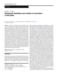
In Figure 3 we plot the logarithmic st<strong>and</strong>ard<br />
where m is probably a rather small number, deviation B <strong>and</strong> the coefficient "a," against N,<br />
without committing ourselves immediately to an using semi-logarithmic plotting. In Figure 4 we<br />
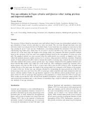
estimate <strong>of</strong> m. '<strong>The</strong>n the modal species will have plot the value <strong>of</strong> R, or half-ranges against N.<br />
nir individuals per species, ant1 the coinmonest It appears that R , is nearly a rectilinear funcwill<br />
have about mr'. In equatloll 13 ) we have tion <strong>of</strong> log N. In Figure 5 we plot r, r2, <strong>and</strong> I/m<br />
denoted mr2 by the symbol Yo.<br />
<strong>The</strong> total nutnber <strong>of</strong> Individuals in the whole<br />
ensemble is<br />
as functions <strong>of</strong> S, log-log ploting.<br />
are nearly straight.<br />
All 3 lines<br />
I = $it'; Yo/%= Xv'G Pos<br />
whence I/m = %v/Gr3 5 = 1.25 r2 0 (9)<br />
This value <strong>of</strong> Ijnl, as a function <strong>of</strong> the total number<br />
<strong>of</strong> species N, is given in the last column <strong>of</strong><br />
Table I.<br />
N I. No. <strong>of</strong> Swri.<br />
in Enunbk)<br />
FIG. 3. <strong>The</strong> relation between the coefficient "a" in<br />
equation 7, or the st<strong>and</strong>ard deviation a, <strong>and</strong> the total<br />
number <strong>of</strong> species iS) in the ensemble. (Computed relationchip)<br />
FIG.2. <strong>The</strong> relation between the number <strong>of</strong> species<br />
(Y,) in the modal octave <strong>and</strong> the total number <strong>of</strong> species<br />
(Nj in the ensemble. <strong>The</strong> solid line is the computed<br />
relationship from equation 18, <strong>and</strong> is pure theory. <strong>The</strong><br />
obser~ed points are taken from Tahle 11.<br />
In Figure 2 we have plotted yo as a function <strong>of</strong><br />
N, using "log-log" plotting. <strong>The</strong> curve is substantiall?<br />
a straight line. Observed points froin<br />
earlier work, <strong>and</strong> from computations made on<br />
the estimates <strong>of</strong> Fisher <strong>and</strong> <strong>of</strong> hferikallio, are<br />
N L. NI<br />
d Spwie~In th. EnIembhsl<br />
FIG.4. Half-range (2R,,,) as a function <strong>of</strong> N, the<br />
total number <strong>of</strong> species. <strong>The</strong> "Range" is the number <strong>of</strong><br />
octaves n-hich the finite distribution may be expected to<br />
cover.
1% FRANK W. PRESTON Ecology, Val. 43, No. 2<br />
FIG.5. <strong>The</strong> relation <strong>of</strong> r, r" <strong>and</strong> I/m to N. Here r<br />
is the value <strong>of</strong> 2 R,,,, Iim is the total number <strong>of</strong> individuals<br />
divided by that minimum number <strong>of</strong> individuals<br />
(m) that may be assumed necessary to keep a species in<br />
existence, <strong>and</strong> N is the total number <strong>of</strong> species in the<br />
ensemble.<br />
<strong>The</strong> equations <strong>of</strong> these straight lines, as determined<br />
by a least-squares fitting to the data<br />
<strong>of</strong> Table I are<br />
log r = 1.872 log N - 0.875 (10)<br />
log r2 = 3.745 log N - 1.751 (11)<br />
log I/m = 3.821 log N - 1.21 (12).<br />
<strong>The</strong>se equations are, as we have seen, all intimately<br />
connected, <strong>and</strong> if one has to be modified,<br />
all must.<br />
Note that these equations are only approximations,<br />
because the lines are not quite straight.<br />
Equations (10) <strong>and</strong> i11) are probably close<br />
enough for any purposes that I can foresee ; equation<br />
(121, particularly in its inverted form where<br />
it relates log N with log (I/rn), may usefully be<br />
modified slightly for different ranges <strong>of</strong> the value<br />
<strong>of</strong> ?S (See below, under "<strong>The</strong> Species-Area<br />
Curve.").<br />
<strong>The</strong> relation betzeleen I altd N in a<br />
cowtplete ensewtble<br />
We have, in equation (12) a relation between<br />
I <strong>and</strong> N if we can make a reasonable estimate <strong>of</strong><br />
the value <strong>of</strong> m. We have tentatively identified tn<br />
as the number <strong>of</strong> individuals or pairs in the rarest<br />
species <strong>and</strong>, since species are all the time being<br />
exterminated, we may expect that 111 will be a<br />
number not far from unity. In practice we <strong>of</strong>ten<br />
find it so as shown below. Eut a full discussion <strong>of</strong><br />
this would involve many biological considerations.<br />
For instance we find in practice that m is frequently<br />
less, even appreciably less, than unity, <strong>and</strong><br />
the temporary interpretation we have given then<br />
has no meaning. Another, related, meaning can<br />
be given to m but the simplest interpretation for<br />
the present is a purely mathematical one. Any 2<br />
<strong>of</strong> the 3 quantities N, p,, <strong>and</strong> u (or "a"), define<br />
the size <strong>and</strong> shape <strong>of</strong> the Species-Curve, but they<br />
do not define its position along the axis <strong>of</strong> x, i.e.<br />
<strong>of</strong> R. <strong>The</strong> quantity "mu specifies this position.<br />
It thus determines not merely the number <strong>of</strong> individuals<br />
theoretically representing the rarest<br />
species, but also the number <strong>of</strong> individuals representing<br />
any <strong>of</strong> the other species, including the<br />
commonest. In consequence, the relation is really<br />
between (I/m) <strong>and</strong> N, not between I <strong>and</strong> N<br />
directly, but if we know. or can estimate, I <strong>and</strong><br />
N, we can get an estimate <strong>of</strong> m.<br />
<strong>The</strong> Species-Area eqzratiotz<br />
<strong>The</strong>re is one other formula that may be useful<br />
to us. In some cases we may regard individuals<br />
(or pairs <strong>of</strong> birds), as being distributed uniformly,<br />
statistically speaking, over wide areas. Let the<br />
density <strong>of</strong> individuals (or pairs) be p per acre.<br />
<strong>The</strong>n the formula<br />
gives the number <strong>of</strong> individuals or pairs to be ex-<br />
pected on an area <strong>of</strong> A acres. <br />
IVe can substitute this in equation (12) <strong>and</strong> ob- <br />
tain <br />
log N = 0.262 log (p A/m) + 0.316 (14)<br />
AT = 2.07 (p,!m) ,0262<br />
.0?62<br />
(15)<br />
This is the Species-Area Equation under<br />
"ideal" conditions such that the area we consider<br />
is populated with a complete, not a truncated,<br />
lognorn~al ensemble, <strong>and</strong> that the density <strong>of</strong> the<br />
population (p) does not change substantially over<br />
the range oi areas we are considering. <strong>The</strong> first<br />
stipulatioil is important because in contiguous<br />
areas, for which Species-Area Curves are <strong>of</strong>ten<br />
propounded (,<strong>and</strong> this includes nly OWTI con~panion<br />
paper on "Time <strong>and</strong> Space <strong>and</strong> the Variation <strong>of</strong><br />
Species" j, the smaller areas act much like<br />
"samples" <strong>of</strong> larger ones.<br />
If we are dealing with isolates that take the<br />
form <strong>of</strong> complete canonical ensembles, <strong>and</strong> if p<br />
<strong>and</strong> in are substantially unchanged from isolate to<br />
isolate, then equation (15j may be written.
Spring 1962<br />
700<br />
CANONICAL<br />
<strong>and</strong> since, 0.262 is not far from 1/4, this may<br />
be written<br />
E
'<br />
synlmetrical distribution, <strong>of</strong> which we showed<br />
examples in Preston ( 1948).<br />
17'e have shown above the mathelnatical consequences<br />
<strong>of</strong> 2 assumptions; viz, that abundance is<br />
typically distributed lognormally among species,<br />
<strong>and</strong> that this distribtuion is <strong>Canonical</strong> in the sense<br />
that not all lognormals meet the requirement. but<br />
only those in which a definite relation exists<br />
between the nunlber <strong>of</strong> species, (N), the number<br />
<strong>of</strong> species in the modal octave (yo), <strong>and</strong> the logarithnlic<br />
st<strong>and</strong>ard deviation (3). 71re now consider<br />
what degree <strong>of</strong> confirmation or refutation is available<br />
from observation.<br />
Thc relatiztt? corzstancy <strong>of</strong> o <strong>and</strong> "a"<br />
In any Gaussian distribution or. in our case,<br />
any lognormal distribution, we have from equation<br />
(S),<br />
That is, the total number <strong>of</strong> species in the "universe"<br />
is proportional to the product <strong>of</strong> the number<br />
<strong>of</strong> species in the 111odal octave <strong>and</strong> the logarithmic<br />
st<strong>and</strong>ard deviation. .As the number oi<br />
species increases, yo or o, or both, must increase.<br />
\\-hen the distribution is canonical both increase,<br />
but 3 increases only slowly while yo increases<br />
rapidly. In fact if we double N,J, increases by<br />
about 857c, but o by only 870 in the range <strong>of</strong> most<br />
interest to us.<br />
Similar-1~-, since "a," the "modulus <strong>of</strong> precision,"<br />
is related to 3 by the formula u' =<br />
1/(2a2), "a" also is relatively constant. This is<br />
what we found in Preston ( 1915).<br />
Tlli,tllt~iri~rical eullc~s <strong>of</strong> "a" aftd o<br />
Kot only are these values relatively constant<br />
over the accessible range <strong>of</strong> 7 alues <strong>of</strong> N,but Table<br />
111 shows that, in this range, where S averages<br />
perhaps two or three hundred species, "a" is about<br />
0.175 <strong>and</strong> 3 is about 3 octaves, or something like<br />
one <strong>and</strong> a fifth orders <strong>of</strong> magnitude.<br />
Xoxv, referring to Table I. vie see that for 311<br />
species we should theoretically ha1.e an average<br />
value <strong>of</strong> "a" <strong>of</strong> about 0 169. This agreement is<br />
close, perhaps fortuitously so (see below on contagious<br />
distributions). but it warrants a few com-<br />
~tlents.<br />
<strong>The</strong> only attempts to get a picture or' the cornplete<br />
ensemble by direct observation are those <strong>of</strong><br />
Fisher (1952) <strong>and</strong> Xerikallio ( 1958 ). <strong>The</strong>re<br />
are considerable difficulties with the experimental<br />
work <strong>and</strong> soine uncertainties, sotne <strong>of</strong> which the<br />
authors have indicated. <strong>The</strong> other results come<br />
PRESTOS Ecology, Vol. 43, No, 2<br />
TABLE111. (Ohserved Relationships). N is the number<br />
<strong>of</strong> species estimated, on the basis <strong>of</strong> the sample, to be<br />
present in the total "universe" or "population": yo is the<br />
number <strong>of</strong> species in the modal octave, <strong>and</strong> "a" is the<br />
"n~odulus<strong>of</strong> precision" <strong>of</strong> the lognormal distribution<br />
I<br />
Reference<br />
Eaunders (birds) 91 10 Preston 1948<br />
Diri.:m<strong>of</strong>hs~~ . . 410 48 Preston 1948<br />
Dirks (female moths'] . .. 383 42 Preston 1948<br />
WiUiam (nioths! . . . . 273 35 Preston 1948<br />
King (moths! . . . . . . . . , 277 33 Preston 194s<br />
Seamans !moths; . . . 332 3U Preston 194.8<br />
Maryl<strong>and</strong> birds . . . . . . . 233 28 Preston 1957<br />
Kation-aide bud count.. . 530 ; 38 Preston 1959<br />
Nearctic estimate . ... . . . , 600 Praton 1948<br />
L<strong>and</strong> Birds <strong>of</strong> Engl<strong>and</strong><br />
Flsher 1952<br />
!vIerikalllo 1958<br />
from estimates <strong>of</strong> what the "universe" is like as<br />
a result <strong>of</strong> studying a sample. Indeed neither<br />
Fisher nor hlerikallio was studying a perfect<br />
"isolate," though they approximated it. <strong>The</strong><br />
sample theoretically has the same modal height<br />
<strong>and</strong> the same dispersion as the universe, <strong>and</strong> it<br />
has also a 3rd variable, the position <strong>of</strong> the "I'eilline,"<br />
or what is the same thing in the end, the<br />
abscissa <strong>of</strong> the mode. This 3rd disposal~le variable<br />
makes our estimates <strong>of</strong> the other 2 tnore<br />
uncertain than they would otherwise be, <strong>and</strong><br />
therefore agreement in our estimate <strong>of</strong> "a" or s<br />
\vithin abut 67% seems in part fortuitous. For<br />
a discussion <strong>of</strong> the fitting <strong>of</strong> truncated Gaussian<br />
distributions see Hald (1952,). Furthemore, u+en<br />
we are dealing with truncated ensembles, we do not<br />
directly observe the value <strong>of</strong> K, the total nunlber<br />
<strong>of</strong> species, but have to estinlate it from the sample.<br />
This throws a further strain npon the interpretation<br />
<strong>of</strong> our observations.<br />
Thi,rclatio~l l~etnvi.~~ !I, <strong>and</strong><br />
To the extent that ~ve find the correct relationship<br />
bet\\-een o <strong>and</strong> N \x7e must necessarily find a<br />
correspondingly correct relationship between yo<br />
<strong>and</strong> N but, since 3 is SO nearly constant over the<br />
observable range <strong>of</strong> N while yo varies rather rapidly,<br />
yo may throw some further light on the<br />
matter. Table I11 gives the observed values <strong>of</strong> yo<br />
for various T alues <strong>of</strong> K,most <strong>of</strong> which are estimated<br />
from inconlplete or truncated distributions :<br />
Figure 7 shows the data in graphical for~n. It<br />
should be once more emphasized that the line is<br />
purel? theoretical. <strong>The</strong> s~l~all circles represent<br />
observed points from Tal~le 111. <strong>The</strong> line is not<br />
"fitted" to the points <strong>and</strong> then extrapolated; the<br />
line is from theory, the points fronl observation.<br />
But it will be observed that the line passes neatly<br />
among the observed points wl~icli lie in a narrow
Spring 1962<br />
CANONICAL DISTRIBUTION<br />
b<strong>and</strong> straddling the line so that if u7e did "fit"<br />
a line to the observations it would not be very<br />
different from the theoretical one. <strong>The</strong> observed<br />
points not only lie reasonably near the line, but<br />
they parallel its course. This gives us an additional<br />
point <strong>of</strong> agreement between theory <strong>and</strong> observation,<br />
bejond what we get from considering<br />
the relationship <strong>of</strong> o <strong>and</strong> N.<br />
Tlze relation bctween N <strong>and</strong> I in a complete<br />
elzsprnblc<br />
Here we exclude discussion <strong>of</strong> tlte relation between<br />
N arid I in "san~ples." <strong>The</strong> best way to<br />
get complete enseml~les is probably to deal with<br />
"isolates" such as the fauna <strong>and</strong> flora <strong>of</strong> isl<strong>and</strong>s<br />
\vhich are in internal equilibrium, but not necessarily<br />
in equilibrium with, or even appreciably<br />
affected by. the populations <strong>of</strong> other l<strong>and</strong> masses.<br />
However, so far as 1 know, we have no counts<br />
<strong>of</strong> indi~iduals for such isl<strong>and</strong>s, nor even good<br />
estimates <strong>of</strong> the numbers <strong>of</strong> individuals. Fortunately<br />
when our areas beconle reasonably large,<br />
<strong>of</strong> the order perhaps <strong>of</strong> 50,000 to 100,000 square<br />
miles, the distribution begins to approximate<br />
closely to that <strong>of</strong> a complete ensemble (in the case<br />
<strong>of</strong> birds) even though the area is in intimate<br />
contact with neighboring l<strong>and</strong> areas. \Ve have<br />
at least 2 fairly good estimates <strong>of</strong> the number<br />
<strong>of</strong> species <strong>and</strong> <strong>of</strong> individuals on such areas : James<br />
Fisher's (1952') estimate <strong>of</strong> the lam' birds <strong>of</strong><br />
Engl<strong>and</strong> <strong>and</strong> 11-ales, <strong>and</strong> Alerikallio's (19581<br />
estimate <strong>of</strong> the breeding birds <strong>of</strong> Finl<strong>and</strong>.<br />
TI~Elnnd birds <strong>of</strong> Engl<strong>and</strong> <strong>and</strong> Walcs<br />
Fisher lists some 142 l<strong>and</strong> birds as regular<br />
1)reeding specles, <strong>and</strong> the distribution 1001~sreasonably<br />
complete <strong>and</strong> symmetrical (see h~s Figure<br />
I). From our equation (12), vie compute that<br />
I/m = 10,000,000 very closely. Fisher estimates<br />
that I 1s 63,000,030~)rdizini~rcrls,hence n~ should<br />
be al~proxin~ately 6 indi\iduals or 3 pairs. This<br />
15, I think, a reasonal~le estimate <strong>of</strong> the nutnher <strong>of</strong><br />
pairs <strong>of</strong> the rarest regularly-breeding species.<br />
<strong>The</strong> xalue <strong>of</strong> r' maj be computed fro111 iorrnula<br />
( 11) <strong>and</strong> comes out very close to 2,000,000 Tl~en<br />
mr3 = 6.3 X 2 X lo0 = 12.6 million indlx ]duals<br />
Fisher gixes a value <strong>of</strong> 10 million approsin~ately,<br />
io again the agreenlent is good <strong>The</strong> I alue <strong>of</strong> r<br />
inay he computed from formula (10) or taken as<br />
the square root <strong>of</strong> 2 ~nillioil. <strong>The</strong>n we get mr =<br />
8.90 individuals per species in the modal octave.<br />
Our computation from his data (which are not<br />
given in great detail) is 8,500. <strong>The</strong> agreement is<br />
almost too good.<br />
Tllc breeding birds <strong>of</strong> Finl<strong>and</strong><br />
193<br />
Merikallio (1958) lists about 204 species. On<br />
this basis we should expect I/m to be about 41<br />
million. blerikallio gives a value <strong>of</strong> I <strong>of</strong> 31 million<br />
pairs, hence our con~putation suggests in this<br />
case that m is about one pair (0.76 pairs). We<br />
can also compute that r = 2,810, whence mr =<br />
2.1 X 10³ for the modal species <strong>and</strong> mr2 = 6.0 X<br />
10Vor the con~monest. <strong>The</strong> figure Alerikallio<br />
gives for his commonest species is 5.7 X lo6pairs,<br />
where once more the agreement is accidentally<br />
too good, <strong>and</strong> our computation from his figure<br />
gives the modal representation as 4.26 X lo3,<br />
which is fair.<br />
<strong>The</strong> relation between N <strong>and</strong> A: the Species-Area<br />
Czi~vefor conlplete Catlonical e~zse~llblcs<br />
In general there can be no complete count <strong>of</strong><br />
indix iduals on areas large enough to approximate<br />
complete ensembles. Both Fisher <strong>and</strong> Merikallio<br />
use methods <strong>of</strong> estimating, not counting, individuals<br />
except for the rarest species. <strong>The</strong>ir<br />
nlethods could <strong>of</strong> course be extended to other<br />
areas <strong>and</strong> other taxonomic groups <strong>and</strong> it might<br />
then be seen how nearly the theory fits the obaervations.<br />
1Ve can however assume that in certain parts<br />
<strong>of</strong> the world we have isolates, or near-isolates, <strong>of</strong><br />
some taxononlic groups on isl<strong>and</strong>s <strong>of</strong> different<br />
sizes between ~vhich there is very Iitnited floral<br />
or faunal interchange, <strong>and</strong> that on each <strong>of</strong> these<br />
isl<strong>and</strong>s there may be a fair approximation to a<br />
canonical distribution. <strong>The</strong>se isl<strong>and</strong>s ought to be<br />
titimerous enough for us to strike a reasonably<br />
good statistical correlation; they should be siinilar<br />
cliinatically <strong>and</strong> not too dissimilar in legetation<br />
cover <strong>and</strong> soil. <strong>The</strong>re are 2 obvious groups<br />
<strong>of</strong> such isl<strong>and</strong>s, the East Indies <strong>and</strong> the ]irest, <strong>and</strong><br />
there are taxonomic groups such as l<strong>and</strong> mammals,<br />
l<strong>and</strong> reptiles, <strong>and</strong> amphibia that do not readily<br />
cross stretches <strong>of</strong> sea. Birtls qualify partially,<br />
<strong>and</strong> are usually better knoxvn. Unfortunately,<br />
the number <strong>of</strong> species on the siilaller islalids is<br />
~rsuallj- far below what we like for statistical<br />
work. Elsewhere (Preston 1957) I have suggested<br />
that we ought to have something like 200<br />
species, <strong>and</strong> this is out <strong>of</strong> the question for the<br />
groups mentioned. llTe must according15 do the<br />
best ne can with smaller numbers.<br />
Thr 111a11~wlulsthe <strong>of</strong> East Iudics<br />
Darlington (1957, p. 480) discusses the mammals<br />
<strong>of</strong> Sumatra, Borneo <strong>and</strong> Java. <strong>The</strong>se isl<strong>and</strong>s<br />
are comparable in latitude <strong>and</strong> climate (a matter<br />
that cannot l~e neglected) <strong>and</strong> their areas are
given as 167,000: 290,000; <strong>and</strong> 49,000 square<br />
miles respectively, while their "units" <strong>of</strong> mammals<br />
are 55, 47, <strong>and</strong> 33. "Units" in this case are<br />
a mixture <strong>of</strong> species <strong>and</strong> genera. Striking an<br />
average <strong>of</strong> the 2 larger isl<strong>and</strong>s gives us an<br />
imaginary isl<strong>and</strong> 228,000 mi2 <strong>and</strong> 51 species.<br />
Comparing this with the smaller isl<strong>and</strong> <strong>of</strong> Java by<br />
means <strong>of</strong> the formula<br />
z = log (NJNz) /log (A1/A2) (from eq. (18) ) (20)<br />
where the suffix 1 applies to the one isl<strong>and</strong> <strong>and</strong><br />
the suffix 2 to the other, we find that<br />
z = 0.28<br />
which is very close to what is called for by the<br />
theory <strong>of</strong> Equation (20).<br />
Awpllibia <strong>and</strong> reptiles <strong>of</strong> the West Indies<br />
Darlington (1957, p. 383) in discussing the<br />
Atlura <strong>and</strong> the lizards <strong>and</strong> snakes <strong>of</strong> Cuba, Hispaniola,<br />
Jamaica <strong>and</strong> Puerto Rico, with some<br />
support from the small isl<strong>and</strong>s <strong>of</strong> Montserrat <strong>and</strong><br />
Saha in the Lesser Antilles, concludes that "diisi<br />
ion <strong>of</strong> area by ten divides the fauna by two."<br />
(<strong>The</strong> "herps" on 40,000 mi2 total about 80, <strong>and</strong><br />
on 4,000 mi2 about 40.) Darlington's statement<br />
implies that<br />
z = log 2/log 10 = log 2 = 0.301<br />
which is quite close to the theoretical value <strong>of</strong><br />
0.28. <strong>The</strong> smaller isl<strong>and</strong>s support Darlington's<br />
views, but since the number <strong>of</strong> species is very<br />
small, neither agreement nor disagreement would<br />
carry much weight.<br />
It may be noted that if we take frogs <strong>and</strong> toads<br />
alone, since the legitimacy <strong>of</strong> lumping these with<br />
lizards <strong>and</strong> snakes may be questioned, we have<br />
an average <strong>of</strong> 25% species on the 2 larger isl<strong>and</strong>s,<br />
with an average <strong>of</strong> 35,000 mi2, <strong>and</strong> an average <strong>of</strong><br />
14% species on the two smaller isl<strong>and</strong>s, with an<br />
average <strong>of</strong> 4000 mi" <strong>The</strong> computation then gives<br />
z =0.26, which is also the theoretical value. <strong>The</strong><br />
reptiles (snakes <strong>and</strong> lizards combined) give a<br />
value <strong>of</strong> 0.318; the lizards alone give a value <strong>of</strong><br />
0.294. <strong>The</strong> snakes are too few to be used safely<br />
for a caculation.<br />
PRESTOS Ecology, vol. 43. No. 2<br />
to canonical lognorinals <strong>and</strong> the exponent z may<br />
be expected to approach 0.26-0.28, the theoretical<br />
value, or to be a little lower.<br />
Bond (1936 <strong>and</strong> 1956, with supplements) has<br />
given detailed accounts <strong>of</strong> these birds, from which<br />
Ī attempted to compile a list <strong>of</strong> the breeding<br />
species <strong>of</strong> all the major isl<strong>and</strong>s <strong>and</strong> a number <strong>of</strong><br />
the smaller ones. <strong>The</strong> areas I took from the<br />
Encyclopedia Britannica, edition <strong>of</strong> 1949. In the<br />
case <strong>of</strong> a few species, while Bond leaves no doubt<br />
that they breed within the West Indies, there may<br />
be some uncertainty whether they breed regularly<br />
on some <strong>of</strong> the isl<strong>and</strong>s. This is probably unimportant<br />
in the case <strong>of</strong> the major isl<strong>and</strong>s, where<br />
the birds are probably better known, but I may<br />
be in error in connection with some <strong>of</strong> the smaller<br />
ones. In order to permit others to correct me, I<br />
give in Table IV a list <strong>of</strong> the isl<strong>and</strong>s I have used,<br />
their areas <strong>and</strong> my estimates <strong>of</strong> the numbers <strong>of</strong><br />
breeding species <strong>of</strong> birds, <strong>and</strong> in Figure 7 I have<br />
graphed the results. Note that I have excluded<br />
introduced species. Note also that the Isle <strong>of</strong><br />
Pines has an abnormally rich fauna for its size.<br />
This probably comes about from its not being an<br />
"isolate," but rather a "sampleJ' <strong>of</strong> Cuba, probably<br />
a truncated distribution.<br />
<strong>The</strong> line is not a calculated regression line, but<br />
TABLEI\'.<br />
Birds oi the West Indies<br />
I<br />
I<br />
Breeding Species<br />
Isl<strong>and</strong> Area in Square Miles <strong>of</strong> Birds<br />
Cuba ...........<br />
(Isle <strong>of</strong> Pines). ...<br />
Hispaniola. ......<br />
Jamaica. . .......<br />
Puerto Rim. ....<br />
Bahamas. .......<br />
Virgin Isl<strong>and</strong>s. ...<br />
Guadalupe.......<br />
Dominica. .......<br />
St. Luoia.. ......<br />
St. Vincent. . ....<br />
Grenada. ........<br />
Bivds oj the W-est Indies<br />
<strong>The</strong> populations <strong>of</strong> birds, particularly seafowl,<br />
on the various isl<strong>and</strong>s <strong>of</strong> the West Indies are<br />
probably somewhat less isolated from one another<br />
than the frogs <strong>and</strong> lizards. On the other h<strong>and</strong><br />
there is quite likely not much gene-flow among a<br />
large proportion <strong>of</strong> the l<strong>and</strong>-birds. <strong>The</strong> populations<br />
<strong>of</strong> each isl<strong>and</strong> may therefore approximate<br />
LOG (Area in sqwra miles)<br />
FIG.7. Birds <strong>of</strong> the West Indies: Species-Area Curve.<br />
<strong>The</strong> abscissa gives the areas <strong>of</strong> the various isl<strong>and</strong>s; the<br />
ordinate is the total nutnber <strong>of</strong> hird species breeding on<br />
each isl<strong>and</strong>.
Spring 1962<br />
CANONICAL Dl[STRIBUTION<br />
is drawn "by eye" <strong>and</strong> seems reasonable; it is<br />
scarcely worth more refinement in view <strong>of</strong> the<br />
errors I may have made in my estimates or the<br />
general question <strong>of</strong> how legitimate it may be to<br />
include seafowl in a study <strong>of</strong> "isolates." Its slope<br />
corresponds to z = 0.24, which seems to agree<br />
well with expectations.<br />
Bird.\. <strong>of</strong> the East Indies<br />
<strong>The</strong> "East Indies" here includes 2 or 3 isl<strong>and</strong>s<br />
<strong>of</strong> the Sunda Shelf, <strong>and</strong> several other isl<strong>and</strong>s not<br />
strictly on the shelf or even part <strong>of</strong> the same<br />
zoogeographical province, <strong>and</strong> one isl<strong>and</strong>, Ceylon,<br />
far removed to the west. Howeyer, the isl<strong>and</strong>s<br />
are a11 essentially tropical <strong>and</strong> climatically not too<br />
dissimilar. I have depended heavily on information<br />
supplied by Dr. Kenneth Parkes who has<br />
used, besides his own knowledge, the findings <strong>of</strong><br />
Delacour <strong>and</strong> Mayr. <strong>The</strong> 1949 Edition <strong>of</strong> the<br />
Encyclopedia Britannica gives somewhat different<br />
counts <strong>of</strong> species.<br />
A list <strong>of</strong> the isl<strong>and</strong>s with their areas <strong>and</strong> breeding<br />
species as given in Table V, <strong>and</strong> the results are<br />
graphed in Figure 8. <strong>The</strong> slope <strong>of</strong> the curve<br />
is z = 0.288, close to the theoretical value which<br />
in this case should be about 0.27. <strong>The</strong> curve<br />
is drawn "by eye," but seems likely to be as close<br />
TABIZV.<br />
Isl<strong>and</strong><br />
Breeding birds <strong>of</strong> some East<br />
1<br />
Indian isl<strong>and</strong>s<br />
I<br />
13reecl~gi:gcies<br />
Area in Square Miles<br />
-<br />
Sew Guinea. ..... 312,000 540<br />
Borneo. .......... 290,000 430<br />
Phillipines (excluding<br />
Palawan) 144,000 368 <br />
Celebes. ......... 70,000 220 <br />
Java. ............ 48,000 337 <br />
Ceylon. .......... 25,000 232 <br />
Palawan. ........ 4,500 111 <br />
Flores. ........... 8,870 143 <br />
Timor.. .......... 300 X 60 = 18,000 137 <br />
Sumba. .......... 4,600 108 (or 103) <br />
1 I I I I I I<br />
30 4.0 50 60<br />
LOG (Area In Square Mllea I<br />
FIG.8. Birds <strong>of</strong> the East Indies: Species-Area Curve.<br />
<strong>The</strong> abscissa gives the areas <strong>of</strong> the various isl<strong>and</strong>s; the<br />
ordinate is the total number <strong>of</strong> bird species breeding on<br />
each isl<strong>and</strong>.<br />
195<br />
as the observational evidence warrants. Good<br />
counts on some smaller isl<strong>and</strong>s might help but, in<br />
view <strong>of</strong> differences <strong>of</strong> opinion among taxonomists<br />
as to what constitutes a valid species, <strong>and</strong> in view<br />
also <strong>of</strong> the fact that with small isl<strong>and</strong>s statistical<br />
fluctuations or "errors" are likely to be important,<br />
I am not sure that much would be gained.<br />
It may be noted that Java is rich for its size,<br />
while Celebes is poor. Ceylon is relatively<br />
"rich," but it may be acting to some extent as a<br />
sample <strong>of</strong> India <strong>and</strong> thus be somewhat enriched.<br />
New Guinea is famous for its wealth <strong>of</strong> species<br />
but some fraction <strong>of</strong> these may be an enrichment<br />
from the Australian mainl<strong>and</strong>. Mayr 11934)<br />
comments that Timor is poor in birds, being both<br />
peripheral <strong>and</strong> arid.<br />
<strong>The</strong> birds <strong>of</strong> Mada.gascar <strong>and</strong> the Comoro Isl<strong>and</strong>s<br />
Madagascar is one <strong>of</strong> the large isl<strong>and</strong>s <strong>of</strong> the<br />
world, with an area <strong>of</strong> 229,000 mi" <strong>The</strong> Cotnoro<br />
Isl<strong>and</strong>s lie <strong>of</strong>f its northeast coast, in the Mozambique<br />
Channel, in Latitude 12"s. <strong>The</strong>y are 4 small<br />
isl<strong>and</strong>s, averaging about 200 mihpiece, <strong>and</strong><br />
have received their bird fauna predominantly from<br />
llladagascar (Benson 1960). hladagascar has apparently<br />
been an isolated isl<strong>and</strong> since early<br />
hlesozoic (Triassic) times while the Comoros<br />
date back to the mid-Tertiary (Miocene) times.<br />
<strong>The</strong> 1949 edition <strong>of</strong> the Encylopeclia Britannica<br />
gives about 260 species <strong>of</strong> birds for Madagascar.<br />
R<strong>and</strong> (1936) gives his estimate as 237 breeding<br />
species. I have comprised on 250. Benson ( 1960,<br />
p. 18) gives the breeding bird tally as follows: on<br />
Gr<strong>and</strong> Comoro (366 square miles), 35 species;<br />
on PvIoheli (83 square miles), 34 species; on<br />
Anjouan (178 square miles), 35 species; on Mayotte<br />
( 170 square miles), 27 species.<br />
lladagascar is roughly a thous<strong>and</strong> times as<br />
large as the average Comoro Isl<strong>and</strong> <strong>and</strong> there are<br />
no isl<strong>and</strong>s <strong>of</strong> intermediate size in the immediate<br />
neighborhood. We can, however, make the assumption<br />
that over the ages, many species <strong>of</strong> birds<br />
from Madagascar, Africa, <strong>and</strong> occasionally elsewhere<br />
have made l<strong>and</strong>falls on the Comoros, <strong>and</strong><br />
that the isl<strong>and</strong>s have as large a number <strong>of</strong> species<br />
as they can support. On that basis we can plot<br />
them on a graph along with the avifauna <strong>of</strong><br />
Plladagascar, arid this has been done in Figure 9.<br />
<strong>The</strong> line has been dram711 by eye, <strong>and</strong> its equation<br />
1s<br />
?J = 7.93 AO?Y<br />
<strong>The</strong> exponent. 0.28, is very slightly above the<br />
theoretical value. <strong>and</strong> the coefficient, 7.95, only a<br />
little below the theoretical value <strong>of</strong> 10, appropriate
190 FRANK W.<br />
I<br />
MADAGASCM 8 THE COUORO ISLANDS<br />
I ,<br />
21 2.0 30 3, .o 1.5 3 0 5'<br />
LOG A I 8n square mllrr l<br />
FIL.9. Birds <strong>of</strong> Madagascar <strong>and</strong> the Conioro Isl<strong>and</strong>s :<br />
Species-.4rea Curve. <strong>The</strong> abscissa gives the areas oi the<br />
various isl<strong>and</strong>s; the ordinate is the total number <strong>of</strong><br />
hird species breeding on each isl<strong>and</strong>.<br />
whet1 A is it1 square niiles <strong>and</strong> p/m is assumed to<br />
be unity.<br />
Tllr l<strong>and</strong> zfrrtebrates <strong>of</strong> islalzds in Lake Michigan<br />
Hatt et al. ( 1935. p. 119j list 12 isl<strong>and</strong>s in Lake<br />
Michigan ranging in area fro111 2.5 acres to 37.400<br />
acres, <strong>and</strong> in species-count <strong>of</strong> l<strong>and</strong> vertebrates from<br />
4 to 120. <strong>The</strong> 2 smallest isl<strong>and</strong>s wit11 8 <strong>and</strong> 4<br />
species respectively are <strong>of</strong> dubious value for our<br />
~~urposes, but the remaining 10 isl<strong>and</strong>s, 11-ith a<br />
minimum <strong>of</strong> 19 ipecies, seem satisfactory. L<strong>and</strong><br />
1-ertehrates are defined as amphibians, reptiles,<br />
birds <strong>and</strong> niatnn~als Tahle 1'1 gives the information.<br />
Figure 10 presents the data in graphical form<br />
for the 10 larger isl<strong>and</strong>s <strong>and</strong> a log-log plot yields<br />
a fair approsimation to a straight line. <strong>The</strong> curve<br />
as tlrann has the equation r\: = 10 Ao2' (where<br />
,Z is it1 acres). This inlplies a high den,ity <strong>of</strong><br />
individual "vertebrate anirnals" compared with<br />
n-hat we encounter among birds. <strong>The</strong> slope, or<br />
PRESTON<br />
Ect:!ogy, \-01.43, NO.2<br />
esponent 0.24, is not far belolv the theoretical<br />
0.27. If we include the 2 lowest points, a very<br />
rluestionable procedure, <strong>and</strong> give them equal<br />
weight with the other points, the slope <strong>of</strong> the<br />
curve increases to about 0.30. Giving them even<br />
a little weight brings the exponent close to the<br />
theoretical value. I am inclined to suspect that<br />
most isl<strong>and</strong>s have achieved a rough approsimation<br />
to internal ecluilibrium, i.e. to a canonical<br />
distribution, but that there is a modest exchange<br />
<strong>of</strong> individuals among the isl<strong>and</strong>s or with the maitll<strong>and</strong>,<br />
perhaps by water in summer or ice it1 winter.<br />
This tends to depress the index slightly below the<br />
value for strict isolates, <strong>and</strong> nlakes the isl<strong>and</strong>s to<br />
some extent "samples" <strong>of</strong> the mai~ll<strong>and</strong>.<br />
Tllc laud pla~tts <strong>of</strong> the Galapagos Isl<strong>and</strong>s<br />
So far \ye hare been consitlering faunas, <strong>and</strong><br />
~t Inaj be well to consider a flora. Iiroeber (1916)<br />
has made a detailed study <strong>of</strong> 18 <strong>of</strong> the Galapagos<br />
Isl<strong>and</strong>s He does not give the areas <strong>of</strong> any <strong>of</strong> the<br />
isl<strong>and</strong>s, <strong>and</strong> I have obtained these fro111 other<br />
sources, which are not always In \ ery exact agreement.<br />
or by estimates fro111 the U S HJ drographic<br />
Sur~ey maps. One small isl<strong>and</strong>, \~,111ch he calls<br />
Brattle. I hare not been able to identify with<br />
assurance, <strong>and</strong> this has therefore been omitted,<br />
reducing our count to 17 isl<strong>and</strong>s. Since we shall<br />
hare occasion to analyse Iiroeber's results further,<br />
I have here included an outline map <strong>of</strong> the isl<strong>and</strong>s<br />
as Fig. 11.<br />
TABLEVI. L<strong>and</strong> vertebrates uf isl<strong>and</strong>s in Lake Michigan<br />
I I I<br />
Area in<br />
Acres Species Area Species Area Species =Ires Species<br />
CULPEPPER 0 50<br />
IM)<br />
J l . . l l , i , , i<br />
SCALE<br />
LAN0 MILES<br />
j WENMAN<br />
I'N<br />
911'W<br />
90.W 89.W<br />
1 1<br />
38lNOLOE TOWER<br />
I<br />
EQUATOR<br />
1<br />
I<br />
1 <br />
I5 1.0 r.5 3.0 15 4 0 4 L w <br />
LOG \ken in ocres)<br />
FIG.10. L<strong>and</strong> Vertebrates <strong>of</strong> Isl<strong>and</strong>s in Lake Michigan:<br />
Species-Area Curve. <strong>The</strong> abscissa gives the areas<br />
<strong>of</strong> the various isl<strong>and</strong>s; the ordinate is the total number oi<br />
bird species breeding on each isl<strong>and</strong>.<br />
FIG.11. Outline map <strong>of</strong> the Galapagos Isl<strong>and</strong>s.<br />
\Ye shall work principally with Kroeber's Table<br />
VI, from which our Table VII has been prepared,
Spring 1962<br />
1 1<br />
11.............. Barrington I .a 48 <br />
12.............. Gardner 0.2 18 <br />
13.............. Bindloe 45 <br />
14.............. Jervis 1.87 47 42 <br />
15.............. TOR-er 4.4 22 <br />
(16).............. (Brattle)<br />
-<br />
(16)<br />
17.............. Wenman 1.8 14 <br />
18.............. Culpepper 0.9 7 <br />
CANONICAL UISTRIBUTIOX<br />
TABLEVII. <strong>The</strong> l<strong>and</strong> plants <strong>of</strong> the Galapagos Isl<strong>and</strong>s tudes. \Ire have floras <strong>and</strong> faunas, <strong>and</strong> anlong<br />
the faunas we have mammals, birds, reptiles, am-<br />
No. Name<br />
Area<br />
phibians, <strong>and</strong> "l<strong>and</strong> vertebrates."<br />
(Sq. mi.) Species<br />
--<br />
Table VIII summarizes our results. It is clear<br />
-<br />
1.............. Albemarle 2249 325 that the average <strong>of</strong> the 7 z-values comes very<br />
2.............. Charles 64 319 close to the theoretical figure. <strong>The</strong> individual de-<br />
3.............. Chatham 195 <br />
4.............. James 203 306 224 partures from this average figure are in general<br />
5.............. Indefatigable 389 193 modest, <strong>and</strong> the agreement map he regarded as<br />
6.............. Abingdon 20 119 <br />
7.............. Duncan 7.1<br />
103 satisfactory. Departures may be expected because<br />
8.............. Narborough 245 80 <strong>of</strong> several factors. For instance, large isl<strong>and</strong>s are<br />
9.. ............ Hood 18 79 more likely to have high mountains, <strong>and</strong> there-<br />
10.............. Seymour<br />
-<br />
1<br />
-<br />
52 <br />
fore special habitats, than small ones, arid then<br />
area alone would not adequately describe the<br />
opportunities for faunas.<br />
cussed below.<br />
197<br />
Other factors are dis-<br />
TABLEVIII. <strong>The</strong> Species-.Area curve ior isolates (<strong>The</strong><br />
coefficient "z" <strong>of</strong> the Species Area Curve-Summary<br />
with an identifying number added for convenience,<br />
<strong>and</strong> with my estimate <strong>of</strong> the area <strong>of</strong> each isl<strong>and</strong><br />
also added. <strong>The</strong>re is a good deal <strong>of</strong> scatter, because<br />
area is not the only factor that decides the<br />
richness <strong>of</strong> faunas <strong>and</strong> floras, <strong>and</strong> accordingly we<br />
have conlputed 2 regression lines, one for the 12<br />
larger isl<strong>and</strong>s <strong>and</strong> one for all 17. <strong>The</strong> two are<br />
scarcely distinguishable but this is a coincidence ;<br />
too much attention should not be paid, as a rule,<br />
to very small populations. <strong>The</strong> regression line<br />
drawn in Figure 12 is the one for the 12 larger<br />
isl<strong>and</strong>s. but the "points" for the others are indicated.<br />
<strong>The</strong> slope <strong>of</strong> this line is z = 0.325, a little<br />
higher than the theoretical value <strong>of</strong> 0.27 or thereabouts.<br />
Szt+~znwry<strong>of</strong> the c-zlal~tes for isolates<br />
We now have 7 independent estimates <strong>of</strong> the<br />
index z <strong>of</strong> Species-Area curves for "isolates." all<br />
<strong>of</strong> them relating to isl<strong>and</strong>s. Some <strong>of</strong> these are<br />
oceanic isl<strong>and</strong>s, some are isl<strong>and</strong>s in a fresh-water<br />
lake, some are in tropical, some in temperate lati-<br />
',,I<br />
11.1111,"<br />
I.UL""IU10" I,. YI,es<br />
FIG.12. Plants <strong>of</strong> the Galapagos Isl<strong>and</strong>s. Species-Area<br />
Curve. <strong>The</strong> abscissa gives the areas <strong>of</strong> the various<br />
isl<strong>and</strong>s; the ordinate is the total number <strong>of</strong> bird species<br />
hreeding on each isl<strong>and</strong>.<br />
Fauna or Flora 1 Locality / z-value Fig. No.<br />
Mammals. ... 1 East lndies 0 280 none<br />
Amphibian <strong>and</strong><br />
Reptiles. ..... West Indles 0.301 none<br />
Birds. .......... West Indies 0.240 7<br />
Birds. ....... East Ind~es 0 333 S<br />
Birds ..........<br />
JIadngascar <strong>and</strong><br />
Comoros 0 280 9<br />
L<strong>and</strong> Vertebrates Isl<strong>and</strong>s in Lahe<br />
LIich~gnn 0 239 10<br />
L<strong>and</strong> Plants / Galapagos Isl<strong>and</strong>s 0.326 12<br />
I Average (<strong>of</strong> i I----0<br />
285<br />
L<strong>and</strong> Plants. ...... Many areas 10,222 13<br />
<strong>The</strong> j4ocr1ering plants <strong>of</strong> the wot*ld<br />
\iVilliams ( 1943131 has plotted on a log-log basis<br />
all the data available to him for flowering plants <strong>of</strong><br />
adequately defined areas, <strong>and</strong> these areas range<br />
from a few square centimeters to the l<strong>and</strong> area<br />
<strong>of</strong> the globe. He has divided tlze information<br />
into 6 categories. the flora <strong>of</strong> arctic, temperate,<br />
subtropical, tropical, <strong>and</strong> desert regions <strong>and</strong> <strong>of</strong><br />
oceanic isl<strong>and</strong>s, <strong>and</strong> he comments that over the<br />
linear portion <strong>of</strong> the graph, which extends from<br />
about 0.1 km2to lo2kn?, '"to double the number <strong>of</strong><br />
species, the area must be increased by thirty-two<br />
times." This may be compared wit11 Darlington's<br />
statement that the area must be increased about<br />
ten-fold. 11-illiams' statement a~noullts to saying<br />
that our exponent z = 0.20 approximately. Williams<br />
is working with the upper boundary <strong>of</strong> his<br />
scatter plot, the boundary between the area where<br />
there are observed points <strong>and</strong> the area where<br />
there are none. It happens that this boundary is<br />
quite well defined <strong>and</strong> Williams marks it with a<br />
broken line. <strong>The</strong> lower boundary on the other
198 FRANK W.<br />
h<strong>and</strong> is nebulous. Williams treats the upper<br />
boundary as a statement <strong>of</strong> optimum conditions,<br />
i.e. as indicating the maximum number <strong>of</strong> species<br />
that can be accommodated on various sizes <strong>of</strong><br />
"quadrat."<br />
<strong>The</strong> slope is actually a little steeper than<br />
17-illiams' estimate ; I make it 0.222. In Figure<br />
13 I ha1.e reproduced all <strong>of</strong> Il'illian~s' points for<br />
LOG (Area in square km.)<br />
FIG. 13. Re-plotting <strong>of</strong> Williams' plants oi many<br />
isl<strong>and</strong>s <strong>and</strong> other areas. Species-Area relationship. <strong>The</strong><br />
upper curve is Williams' upper limit <strong>of</strong> maximum richness.<br />
<strong>The</strong> lower is the regression line for all plotted<br />
points. N is the number <strong>of</strong> species reported from the<br />
various areas.<br />
areas between 0.1 <strong>and</strong> 10Qm" Below this range<br />
many or most <strong>of</strong> the points must refer to<br />
"samples," i.e. to truncated distributions; it is<br />
virtually certain that a large proportion <strong>of</strong> the<br />
remainder do likewise. This gives us 135 points<br />
with which to work. I have drawn 2 lines on<br />
the graph, one marking the boundary as estimated<br />
by eye, <strong>and</strong> the other the regression line <strong>of</strong> "y on<br />
x" (log N on log A) computed by orthodox<br />
methods. <strong>The</strong> 2 lines turn out to have identical<br />
slopes, z = 0.222. <strong>The</strong> equation <strong>of</strong> the regression<br />
line is in fact<br />
&- = ll$ A"2! (21)<br />
log x = 2.0; + 0.222 log -4. (22)<br />
By separating the categories into which Williams<br />
divides his data, it is possible to compute or<br />
estimate values <strong>of</strong> z for the tropical, temperate,<br />
<strong>and</strong> desert floras. I have merely estimated the<br />
slopes <strong>of</strong> the upper boundary lines. For tropical<br />
<strong>and</strong> desert regions, the slope seems to be about<br />
0.25, for temperate regions, 0.22. <strong>The</strong> regression<br />
lines may be a little flatter. In any case they<br />
PRESTON<br />
Ecology, VO~. 43, NO.2<br />
are all roughly similar, <strong>and</strong> all a little below the<br />
theoretical value, which over this range, which<br />
extends to more than 10,000 species, is about<br />
0.265. We may speculate that though, on unit<br />
area we have approximately complete canonical<br />
distributions. yet some samples are truncated,<br />
thus depressing the index below its theoretical<br />
value, from 0.26 down to 0.22. It may be worth<br />
noticing that the depression is by no means so<br />
great as wre found in Preston (1960) for the<br />
bird faunas <strong>of</strong> the Neotropical region (0.16+,1 or<br />
Nearctic (0.12+) where the truncation is presumably<br />
more pronounced.<br />
We may also note that while the statements <strong>of</strong><br />
Darlington <strong>and</strong> Williams, that it takes 10 times,<br />
or 32 times, the area to double the number <strong>of</strong><br />
species, sound considerably at variance, yet when<br />
expressed as an index the difference is only<br />
between 0.22 <strong>and</strong> 0.30. It will not escape notice<br />
that the average <strong>of</strong> these two is 0.26, almost<br />
esactly the theoretical value, but I think this is<br />
accidental.<br />
Our justification for ignoring those areas in<br />
\T'illiams' graph below 0.1 kmvics less in the<br />
fact that Williams himself did so than in the fact<br />
that we here have many counts involving less than<br />
50 species, <strong>and</strong> scarcely any with more than a<br />
hundred, <strong>and</strong> this brings us to about the limit for<br />
satisfactory statistical work. (This restriction<br />
makes it difficult to work with the extensive tabulations<br />
<strong>of</strong> I'estal 1949. However see below.)<br />
<strong>The</strong>re is another calculation we can make, <strong>of</strong> <br />
a solnewhat more risky kind, since the index 0.222 <br />
differs appreciably from the theoretical one <strong>of</strong> <br />
0.262. 1Ve can compute the theoretical number <strong>of</strong> <br />
individuals per square meter <strong>and</strong> see how it agrees <br />
with what Williams has to say on the subject. <br />
<strong>The</strong> regression line not far frotn the middle<br />
<strong>of</strong> the range we have studied gives 1000 species<br />
at about log A = 4.2 or A = 1.0 x 10"m2.<br />
From Table I we should have I/m = 1.47 x 10¹⁰<br />
individuals when S = 1000 species <strong>The</strong>n if we<br />
assume tentatively that m = 1 or thereabouts, this<br />
involves approximately one flov, ering plant to the<br />
square meter, averaged o>er tropical, temperate,<br />
<strong>and</strong> arctic areas. <strong>The</strong> boundary line ~vould give<br />
as ;In<br />
"optimun~" or n~asimum concentration<br />
something like 30 cm2 to a flowering plant.<br />
Williams says, on p. 260, "Available information<br />
indicates that there is about one plant per<br />
square centimeter in temperate grassl<strong>and</strong>, about<br />
one per square meter in woodl<strong>and</strong>, <strong>and</strong> about one<br />
per hundred square meters upwards in semidesert<br />
areas." Thus our estimates fall \$ ell within<br />
the range <strong>of</strong> concentrations given by J~'illiams,<br />
<strong>and</strong> since ne haye evidence that nl can Tary at
Spring 1962<br />
CAI~ONICALDISTRIBUTIOS<br />
least over the range from 10 to 1/10 or rather<br />
more, the agreement can only l~e regarded as<br />
satisfactory.<br />
Summarizin,g this section, we might say that<br />
there are a number <strong>of</strong> cases where the theory <strong>of</strong><br />
isolated canonical ensembles seems to be confirmed<br />
by the exprimental, or observational, evidence;<br />
or at least the observations seem to accord<br />
with the theory.<br />
Introduction<br />
In the previous two sections we examined first<br />
the theory <strong>of</strong> complete canonical ensembles <strong>and</strong><br />
then the available observations on ensembles that<br />
seemed likely to be substantially complete. Under<br />
ideal conditions we think <strong>of</strong> these as "isolates."<br />
Information <strong>of</strong> this sort is rare, <strong>and</strong> in<br />
general we have to content ourselves with<br />
"samples" drawn from a presumably complete<br />
canonical universe. <strong>The</strong> relationship between<br />
sample <strong>and</strong> universe was discussed briefly in<br />
Preston (19483. IVhat we get, if the sample is<br />
a r<strong>and</strong>om one, is a truncated lognorn~al distribution.<br />
To a close approximation the sample has<br />
the same modal height (yo) as the universe, <strong>and</strong><br />
it indicates correctly the logarithmic st<strong>and</strong>ard<br />
deviation (Q). From these figures the total number<br />
<strong>of</strong> species (N) in the unknown universe may<br />
be computed, though we may have observed or<br />
collected, in the sample, only 70 or 80% <strong>of</strong> them.<br />
A large part <strong>of</strong> the field work <strong>of</strong> an ecologist<br />
consists <strong>of</strong> taking samples, so the properties <strong>of</strong><br />
samples have great practical importance. <strong>The</strong><br />
purpose <strong>of</strong> tlie sampling is in nearly all cases to<br />
deduce sonlething about the "population," "universe,"<br />
or "st<strong>and</strong>" or "community" that is being<br />
sampled, so the relation between sample atld universe<br />
is a matter <strong>of</strong> prime concern. Some <strong>of</strong> the<br />
problems that arise are <strong>of</strong> broad scientific interest.<br />
In large samples, which typically should contain<br />
at least a couple <strong>of</strong> hundred species <strong>and</strong> at least<br />
forty or fifty thous<strong>and</strong> individuals, the problems<br />
are largely analytical in nature; in sliiall or very<br />
small samplcs, biological peculiarities, especially<br />
"contagion," positive or negative (See Cole<br />
19461, become very important ; with larger<br />
samples the "contagion" tends to sn~ooth out <strong>and</strong><br />
disappear.<br />
A "sample" ma>- be obtained by catching nloths<br />
in a light trap. Obviously we do not catch all<br />
the moths that are on the wing, <strong>and</strong> it is clear<br />
that we are dealing with a sample, though it is<br />
far from clear what "universe" we are sampling.<br />
It is important not to assume that we know this<br />
199<br />
iron1 general considerations; in particular, in this<br />
instance. we must not assume that it is the population<br />
<strong>of</strong> a definite geographical area. Some <strong>of</strong> the<br />
noctuid <strong>and</strong> hawk moths we catch may be very<br />
strong fliers <strong>and</strong> may have crossed the English<br />
Channel or some larger body <strong>of</strong> water from foreign<br />
parts; some <strong>of</strong> the geonietrids may be very weak<br />
fliers <strong>and</strong> originate entirely close at h<strong>and</strong>. Similar<br />
considerations apply to birds <strong>and</strong> even to plants,<br />
<strong>and</strong> eve11 illore obviously to wind-blown pollen.<br />
<strong>The</strong> universe being sampled is simply what the<br />
sample says it is; it mu5t be ascertained from the<br />
internal evidence, not from assumptions. This<br />
applies to "quadrats" <strong>of</strong> plants. ant1 hence to the<br />
Specie>-Xrea curves there<strong>of</strong>, just as it applies to<br />
moths in a light trap.<br />
Fzmda~nental differences between sample <strong>and</strong> ztniverse<br />
<strong>The</strong>re are 2 very obvious differences between<br />
a sample <strong>and</strong> a universe: first, the ratio <strong>of</strong> species<br />
to individuals is vastly higher in the sample than<br />
in the universe, <strong>and</strong> second, there are vastly more<br />
species represented by a single specimen ("single-<br />
tons" ), or by a fe~v specimens, in the saniple if it<br />
is a "r<strong>and</strong>om" one.<br />
Let us suppose that we have a "fixed" universe<br />
which will not exp<strong>and</strong> as we collect our r<strong>and</strong>om<br />
sample, <strong>and</strong> let us examine our collection as we<br />
collect it.<br />
<strong>The</strong> first moth into a light trap may be one <strong>of</strong><br />
the commonest species, but it is more likely to<br />
be one <strong>of</strong> some other, since the commonest species<br />
is not as plentiful as all the other species<br />
put together; hence it may very well be that at<br />
first we collect half a dozen moths all <strong>of</strong> different<br />
species. Thus Tve accumulate species, at first, as<br />
ralxdly a, \\ e accumulate individuals. -43 we continue<br />
collecting this situation ceases to obtain, <strong>and</strong><br />
after a time the addition <strong>of</strong> new individuals piles<br />
up indefinitely, while the addition <strong>of</strong> a new species<br />
is a rare event. We have reached the point <strong>of</strong><br />
diminishing returns.<br />
In Preston (1948) we showed that doubling the<br />
catch <strong>of</strong> individuals was approximately equivalent<br />
to n-ithdra~ving a graph oi the lognormal distribution<br />
from under a ITeil-line to a distance <strong>of</strong> one<br />
more octave. This is a very close approxin~ation<br />
ior most <strong>of</strong> the cases <strong>of</strong> practical importance, or at<br />
any rate those cases we were considering in 1948.<br />
But actually nithdrawing the graph by one octave<br />
rather more than doubles the count <strong>of</strong> individuals.<br />
Tt doubles the count for all those octaves that<br />
were previously withdrawn <strong>and</strong> it adds in addition<br />
one individual for each species in the new
200 FRANK U'. PRESTON Ecology, Vol. 43, No. 2<br />
octave now unveiled. This modification <strong>of</strong> our<br />
1948 statement is <strong>of</strong> significance only at the beginning<br />
<strong>of</strong> coIlecting.<br />
<strong>The</strong> indc.~. ","' in the ilrrhenizts Eyliafioil. when<br />
collecting at r<strong>and</strong>ol~l jrou1 a jirc-ed zi,ziverse<br />
<strong>The</strong> Arrhenius equation, in ecological work, is<br />
the statement that the number <strong>of</strong> species (N) is<br />
connected with the area (A) by the equation<br />
I<br />
NEOTROPKAL B!RDS<br />
where I< <strong>and</strong> z are constants. This equation is<br />
not given by Arrhenius but is implied 11y his<br />
work. (See Preston 1960). This is <strong>of</strong> the same<br />
form as our equation (16). Note that we are not<br />
referring to that other Arrhenius equation that<br />
concerns the rate <strong>of</strong> chemical reactions <strong>and</strong> their<br />
variation with temperature.<br />
Suppose in our collecting we have begun at the<br />
octave R,,,,, <strong>and</strong> have reached octave R, going<br />
fro111 right to left across our Species-Curve.<br />
<strong>The</strong> number <strong>of</strong> species we have collected is<br />
<strong>The</strong> numl~er <strong>of</strong> i~ldividuals collected is<br />
Let us now collect till the next octave is fully<br />
exposed. <strong>The</strong> additional number <strong>of</strong> species collected<br />
is<br />
<strong>The</strong> additional number <strong>of</strong> individuals collected is<br />
For a given number <strong>of</strong> species (N) in the fixed<br />
universe, we can, provided it is canonical, obtain<br />
the value <strong>of</strong> y a: any octave, <strong>and</strong> also the value <strong>of</strong><br />
I/m.<br />
Assuming that m does not change as we collect,<br />
<strong>and</strong> there is no reason why in a fixed universe it<br />
should, we can compute the index z in the Arrhenius<br />
equation as<br />
1; = (hlog N,/h log I) (See Preston 1960) (27)<br />
This has been done for the case where N =200<br />
species in the universe, <strong>and</strong> where in consequence<br />
rs = 4.07 octaves if the universe is canonical. <strong>The</strong><br />
tabulation is not reproduced here, but in Figure<br />
14 we give a graph <strong>of</strong> the Index z as ordinate<br />
against the percenta,ge <strong>of</strong> species collected. It<br />
PER CENT COWLETIW OF ZW SPECIES UNIVERSE<br />
FIG.14. <strong>The</strong> index "z" <strong>of</strong> the Arrhenius equation ior<br />
a truncated distribution.<br />
will be seen that at first we collect species<br />
as fast as we collect individuals (z = l), but by<br />
the time we have collected 15 or 16 species (7 or<br />
8% <strong>of</strong> the total <strong>of</strong> 200 species available), z has<br />
fallen to 0.6, <strong>and</strong> from this point on it continues<br />
to fall steadily till it reaches z = 0.0 as the last<br />
species is collected.<br />
<strong>The</strong> inconstaucy <strong>of</strong> z<br />
It follows that "z" in the Arrhenius equation<br />
is not by any means a constant under the conditions<br />
we have stipulated, <strong>and</strong> since the argument<br />
applies to increasing sizes <strong>of</strong> quadrat, i.e, to a<br />
species-area curve, as well as to a sample <strong>of</strong><br />
moths in a light trap, it follow-s that a log-log plot<br />
<strong>of</strong> a species-area curve will not give a straight<br />
line, at least not under the stipulated conditions.<br />
<strong>The</strong> reason we sometimes find a fair approximation<br />
to a straight line in the log-log plot is<br />
that, after we reach a certain degree <strong>of</strong> completeness,<br />
the universe begins to exp<strong>and</strong> as fast as the<br />
sample. This seems to happen typically when we<br />
have collected some 75 or 85% <strong>of</strong> the initiallyavailable<br />
species. <strong>The</strong> remaining species are very<br />
rare, <strong>and</strong> it requires a prodigious effort <strong>and</strong> the<br />
capturing <strong>of</strong> innumerable individuals to get these<br />
rarities by strictly r<strong>and</strong>om collecting. We are<br />
likely to obtain a lot <strong>of</strong> "strays," "casuals," <strong>and</strong><br />
"accidentals" before we succeed in netting all the<br />
rare species that are legitimately present.<br />
In Figure 14. IVilliatns index <strong>of</strong> 0.22 would be<br />
reached at 64% completion, but his data probably<br />
relate to a mixture <strong>of</strong> plant-isolates (with a z index<br />
<strong>of</strong> 0.27) <strong>and</strong> <strong>of</strong> "samples" with an index well<br />
below 0.22. <strong>The</strong> index we found (Preston 1%0)<br />
for the neotropical avifauna, z = 0.16, is reached<br />
at 7370 con~pletion, <strong>and</strong> the figure <strong>of</strong> z = 0.12<br />
( nearctic avifauna) is reached at 83% completion.<br />
This last point is at just about one st<strong>and</strong>ard deviation<br />
beyoild the mode. Collecting by r<strong>and</strong>om<br />
methods beyond this point is a rather unpr<strong>of</strong>itable
Spring 1962<br />
procedure; deliberate searching now pays dividends.<br />
Even when the sample-area seems to be well defined<br />
<strong>and</strong> our e net hods systematic rather than<br />
r<strong>and</strong>om, as in determining the breeding birds<br />
<strong>of</strong> a county or some such area, if we succeed in<br />
locating every pair <strong>and</strong> in counting them, we shall,<br />
in general, have a sample rather than a universe.<br />
Usually it will approximate to being a sample<br />
<strong>of</strong> a much larger area, perhaps <strong>of</strong> an area as large<br />
as a state.<br />
From the same data as before we can construct<br />
a Species-Area curve for suct~ samples. Let us<br />
hide the canonical curve completely behind the<br />
veil line, <strong>and</strong> then withdraw it octave by octave.<br />
At each step <strong>of</strong> the withdrawal we add a nunlber<br />
<strong>of</strong> indit-iduals, slightly more than doubling, in<br />
fact, the number we have already counted, as given<br />
by equation (26). A number <strong>of</strong> individuals may<br />
be taken as proportional to an area. At the same<br />
time we add a tlunlber <strong>of</strong> species given by equation<br />
(25). We plot the accumulated area logarithmically<br />
as abscissa, <strong>and</strong> the accumulated<br />
species either arithmetically (Gleason) or Iogarithmically<br />
(Arrhenius) as ordinate. In Figure<br />
15 we have used the latter method <strong>of</strong> plotting.<br />
CAKONICAL DISTRIBUTIOS<br />
201<br />
At the right-h<strong>and</strong> end <strong>of</strong> the curve, we have 3<br />
lines. <strong>The</strong> loviest is the theoretical behavior <strong>of</strong> an<br />
isolate or fixed universe. <strong>The</strong>re are only 200<br />
species all told, so the curve flattens to horizontal<br />
at this level. In practice, however, before we<br />
reach this point the effort to collect the few remaining<br />
rare species by r<strong>and</strong>om methods results,<br />
as aye ha\ e seen, in causing the universe itself to<br />
exp<strong>and</strong>. <strong>The</strong> middle line, therefore, is drawn as<br />
a straight line, tangent to the cunre at about 8070<br />
completion (i.e. when we have collected 160 species)<br />
<strong>and</strong> haying a shape corresponding to z =<br />
0.12. This resembles the situation we encountered<br />
in our study <strong>of</strong> the Species-Area Curve <strong>of</strong> Nearctic<br />
breeding birds (Preston 1960). In that case it<br />
seemed as though initially our universe consisted<br />
<strong>of</strong> soi~~eivherearound 75 or 100 species<br />
<strong>and</strong> I)y the time we had collected 80% <strong>of</strong> them<br />
the universe was exp<strong>and</strong>ing as fast as the sample.<br />
<strong>The</strong> upper line is the corresponding tangent<br />
for the neotropical fauna, with a slope <strong>of</strong> 0.16. As<br />
we go farther to the right (we are not now limited<br />
to the right h<strong>and</strong> end <strong>of</strong> the graph at 200 species)<br />
both <strong>of</strong> these tangents will ultimately curl upwards<br />
in practice, as discussed in Preston (1960).<br />
<strong>The</strong> general appearance <strong>of</strong> the curxes, with the<br />
double-logarithmic or Arrhenius type <strong>of</strong> plotting,<br />
is that <strong>of</strong> a pair <strong>of</strong> more-or-less straight lines<br />
meeting at an obtuse angle, but rounded <strong>of</strong>f one<br />
into the other, the steeper <strong>of</strong> the lines king toward<br />
the left. <strong>The</strong> graph resenlbles fairly well the 2<br />
curves found it1 practice in the previous paper.<br />
5CN.E 02 OCTAVES 0" WUKWS OF M k<br />
Flc. 15. <strong>The</strong>oretical Species-Area curve for samples.<br />
In this figure, as in the previous one, we assume<br />
that the universe initially sampled consists <strong>of</strong> 200<br />
species. <strong>The</strong> left-h<strong>and</strong> end <strong>of</strong> the curve is shown<br />
as a broken line, till we have captured or observed<br />
20 species; below this level we must in practice<br />
expect all sorts <strong>of</strong> erratic results, <strong>and</strong> indeed for<br />
some little distance beyond it. <strong>The</strong> initial part<br />
<strong>of</strong> the curve is fairly straight <strong>and</strong> quite steep, but<br />
not so steep as the limiting tangent, except at the<br />
very origin. This tangent is indicated; it represents<br />
the start where every new specimen is likely<br />
to be <strong>of</strong> a new species. See Preston (1960) for a<br />
discussion <strong>of</strong> such tangents.<br />
Tlrr sizr oi tlzc ~ltzizrerst~ i)l trr112s<strong>of</strong> the pr<strong>of</strong>ierties<br />
<strong>of</strong> the snmple<br />
Hidden heyond the Veil-line <strong>of</strong> our truncated<br />
distribution, which is our sample, are a number<br />
<strong>of</strong> octaves which are needed to complete our universe.<br />
50 far as species are concertled, this<br />
may amount to only a modest addition, hut for<br />
individuals each octave represents a doubling <strong>of</strong><br />
the population. <strong>The</strong> complete universe is therefore<br />
usually many times as large as the sample.<br />
In Table I the quantity x is the half-range in<br />
terms <strong>of</strong> the st<strong>and</strong>ard deviation as unit, i.e. x =<br />
R,,,,/D. To a first approximation, for the cases<br />
we have encountered <strong>and</strong> are likely to encounter<br />
in practice, with N between 200 <strong>and</strong> 800, x is close<br />
to 3.0.<br />
\\-hen we have collected as far as one st<strong>and</strong>ard<br />
deviation beyond the mode, we have accumulated<br />
84% <strong>of</strong> the species in that universe, but we still<br />
lack 2 0 or thereabouts <strong>of</strong> having the complete<br />
curve. Since G is usually around 1 or 5 octaves,<br />
we still lack some 8 or 9 octaves. <strong>The</strong> size <strong>of</strong> the
202 FRANK W. PRESTON Ecology, Val. 43, No. 2<br />
universe is therefore Z8 or Z9 times the size <strong>of</strong> the<br />
sample, or 250 to 500 times as large.<br />
This statement is better put in this form: we<br />
should have to collect 250 to 500 times as many<br />
specitnens before we had a reasonable chance <strong>of</strong><br />
cbllecting one specimen (or pair) <strong>of</strong> the rarest<br />
species. Better yet, the statement is true in its<br />
original form if m = 1, <strong>and</strong> it frequently seems<br />
to be near this.<br />
This would permit us, for instance, to estimate<br />
the overwintering population <strong>of</strong> the birds <strong>of</strong> the<br />
nearctic, using the Audubon Christmas Bird<br />
Counts (Preston 1958). if we consider only those<br />
species that were found by r<strong>and</strong>om methods.<br />
Suppose for the sake <strong>of</strong> illustration, that in a<br />
typical single year about 10' individuals were seen<br />
<strong>and</strong> that these represented 84% <strong>of</strong> the complete<br />
distribution <strong>and</strong> about 500 species. <strong>The</strong>n 0 should<br />
be about -4.5 octaves <strong>and</strong> x about 3.1. <strong>The</strong> end <strong>of</strong><br />
the distribution would be about 9 octaves away,<br />
<strong>and</strong> the total number <strong>of</strong> overwintering individuals<br />
would be about 500 times the size <strong>of</strong> the sample,<br />
or 5 x lo9 birds. (Again we are assuming that<br />
m = 1.) This is roughly equivalent to saying<br />
that, since the nearctic is roughly 4 or 5 X lo9<br />
acres, we have one bird per acre wintering in the<br />
nearctic. <strong>The</strong>y will <strong>of</strong> course be far from uniformly<br />
distributed, most <strong>of</strong> them being along the seacoasts<br />
or the more southern parts <strong>of</strong> the country,<br />
where some acres will be black with redwings <strong>and</strong><br />
starlings. Whether the estimate is fairly close<br />
or sonlewhat high may depend on whether different<br />
parties <strong>of</strong> observers saw the same large flocks<br />
at different places, <strong>and</strong> on various other prob-<br />
lematical matters. <strong>The</strong> computation merely illustrates<br />
the possibility that we may be able, by<br />
more refined methods <strong>and</strong> especially. perhaps, with<br />
a surer kno~vledge <strong>of</strong> the value <strong>of</strong> "m." to estimate<br />
-<br />
the total wintering population.<br />
We can also compute what fraction <strong>of</strong> a population<br />
must be observed or collected in order to<br />
reach the mode, i.e. to collect 50% <strong>of</strong> the species<br />
<strong>and</strong> get at least a rough idea <strong>of</strong> the height <strong>of</strong> the<br />
niode. \\'ith m = 1, this fraction is simply l/r,<br />
which tnay be ascertained from Table I. So,<br />
~vithn po1x1lation oi 200 speciea, we reach the<br />
mode when we have captured or observed 1/2720<br />
<strong>of</strong> the individuals. With 600 species we need to<br />
observe or capture only 1/17,000 <strong>of</strong> the total.<br />
Graphirnl construction<br />
Suppose we have collected beyond the mode<br />
<strong>and</strong> the truncated distributioll appears as shown<br />
in l'ipure 16. From the point A where the curve<br />
intersccts the 1-eil-line, draw a horizontal line to<br />
intersect the curve again at B. From B draw the<br />
LOG, IINDIVIDUALS PER SPECIES)<br />
FIG.16. Maryl<strong>and</strong> State-wide Bird Count: graphical<br />
estimate <strong>of</strong> degree <strong>of</strong> completeness.<br />
~ertical line BB, intersecting the R axis in B1.<br />
Let C1 be the end <strong>of</strong> the finite distribution actually<br />
observed. BICl is the number (R) <strong>of</strong> octaves<br />
theoretically missing to the left <strong>of</strong> A, the curve<br />
being assumed quite symmetrical. <strong>The</strong>n ZR is the<br />
ratio <strong>of</strong> size <strong>of</strong> universe to size <strong>of</strong> sample.<br />
This particular plot is taken from Preston<br />
( 1957 ) <strong>and</strong> represents the State-wide bird counts<br />
<strong>of</strong> llaryl<strong>and</strong>.<br />
Small samples<br />
For our purposes most samples are to be regarded<br />
as small if the number <strong>of</strong> species involved<br />
is less than about a hundred. <strong>The</strong> number <strong>of</strong><br />
individuals may be extraordinarily diverse. If our<br />
ensembles were canonical, the number <strong>of</strong> individuals<br />
for any given number <strong>of</strong> species would<br />
be ascertainable from Table I. But small biological<br />
"u~liverses," are greatly distorted by "con-<br />
tagion." This is stated succinctly by Cain <strong>and</strong><br />
Castro (1959) : Most plants "are more or less<br />
clumped or contagiously distributed" <strong>and</strong> by Hopkins<br />
(1955 ) : "Results support the view that most<br />
plant individuals are aggregated." A recent paper<br />
by Hairston (1959) may almost be regarded as a<br />
warning that contagion or clumping is so general<br />
<strong>and</strong> widespread that it is scarcely worth while<br />
constructing theories about noncontagious distri-<br />
butions. <strong>The</strong> warning is sound, <strong>and</strong> was given<br />
earlier by Cole (1946), who emphasizes the fact<br />
that biological material, m-hetlier animal or vegetable,<br />
is rarely distributed at r<strong>and</strong>om, but is nearly<br />
always more or less "contagiously distributed,"<br />
<strong>and</strong> he examines the possibility <strong>of</strong> h<strong>and</strong>ling such<br />
distributions adequately by mathematical methods.<br />
But whereas Hairston's emphasis is on the<br />
"clumped" distribution, which he believes is characteristic<br />
more particularly <strong>of</strong> the rarer species,<br />
Cole emphasizes that "contagion" can be "positive"<br />
(clumped J or "~legati~e"( over-regularized)<br />
.<br />
-4 great deal cfepends on the nature <strong>of</strong> the bi-<br />
ological material with which one is working, <strong>and</strong><br />
even upon the season <strong>of</strong> the year. Thus in the
Spring 1962<br />
CANONICAL DISTRIBUTION<br />
breeding season most passerine birds are, o~vi~lg <strong>of</strong> individuals without accumulating many speto<br />
their "territorial" propensities, over-regularized<br />
spatially, <strong>and</strong> therefore on a small area they are<br />
over-rqgularized in abundance. (See below, under<br />
Thomas, Hicks, Williams, I'dalkinshaw, etc.) .<br />
cies. Thus, in order to deal at all with the<br />
But in the winter they "flock" <strong>and</strong> become<br />
"clumped," <strong>and</strong> it is not solely the rarer forms<br />
that do this.<br />
Plants are perhaps the most obviously clumped<br />
material, <strong>and</strong> sometimes approximate to pure<br />
cultures, as with Hopkins' (1955) Zostera community.<br />
However, this can be matched among<br />
colonially nesting birds, like Beebe's ( 1924) "pure<br />
culture" <strong>of</strong> boobies in the Galapagos Isl<strong>and</strong>s. or<br />
the Emperor Penguin (Apfertodytes forsteri) in<br />
Antarctica. <strong>The</strong>refore it seems to me that we<br />
are justified in examining the properties <strong>of</strong> r<strong>and</strong>omly<br />
distributed populations, <strong>and</strong> treating them<br />
as a "norm," <strong>and</strong> we nlay treat contagion, whether<br />
positive or negative, as introducing a disturbance,<br />
modification, or perturbation into our calculations.<br />
Notwithst<strong>and</strong>ing Hairston's ( 1959) comment<br />
that, so long as vie are dealing with a single community,<br />
"departure from r<strong>and</strong>omness increases<br />
with sample size," I thillk we are justified in<br />
assuming that in this paper we shall rarely be<br />
dealing .n-it11 a single community, but with what<br />
he calls heterogenous material, in which departure<br />
fro111 r<strong>and</strong>omness decreases with increasing saniple<br />
size. Thus in order to study contagion in our<br />
present context we must examine the properties<br />
<strong>of</strong> rather small samples.<br />
Since in the present paper we are concerned<br />
with abundance-distributions <strong>and</strong> want to know<br />
whether they conforn~ to the lognormal type, <strong>and</strong><br />
in particular to the canonical lognormal, a small<br />
sample for our purposes is primarily one that<br />
has rather few species, say a hundred or less. For<br />
with less than about one hundred we cannot plot<br />
the distribution graphically with much success.<br />
It is true we might use analytical methods rather<br />
than graphical ones, as being more powerful tools,<br />
but statistical fluctuations are not thereby prevented<br />
from confusing the issue, <strong>and</strong> so in Preston<br />
(1957) I suggested that an adequate sample called<br />
for something like a minimum <strong>of</strong> 200 species <strong>and</strong><br />
something like a mitlimum <strong>of</strong> 30,000 individuals.<br />
Very little in the way <strong>of</strong> plant material meets<br />
the requirement <strong>of</strong> 200 species. or eveti 100. <strong>and</strong><br />
much <strong>of</strong> it, in fact most <strong>of</strong> it, appears to have less<br />
than 50, <strong>of</strong>ten much less. <strong>The</strong> individuals may<br />
be very numerous, especially in our northern latitudes<br />
where the floras are poor compared with the<br />
tropics (Cain <strong>and</strong> Castro, 1959) but, because<br />
the majority <strong>of</strong> plant distributions are "positively"<br />
contagious, we have an abnormally high ntltnber<br />
203<br />
published literature on plant distributions, i.e.,<br />
their relative abundances in a "community" or<br />
their Species-Area curves, we have to compile<br />
a tabulation <strong>and</strong> make a graph <strong>of</strong> what to expect <strong>of</strong><br />
samples containing less than 100 species.<br />
Criteria for s~~lall sar?tples<br />
With small samples in this sense, it is easier<br />
<strong>and</strong> perhaps more accurate to reduce them to<br />
graphs, <strong>and</strong> the easiest computation to make concerns<br />
the (logarithmicj st<strong>and</strong>ard deviation o.<br />
<strong>The</strong>refore in Table I9 below we use the methods<br />
TABLEIX. Properties <strong>of</strong> small canonical ensembles<br />
I<br />
I<br />
Number <strong>of</strong> Logarithmic st<strong>and</strong>ard Ratio <strong>of</strong> individuals<br />
species S deviation a (octaves) to species I/N or<br />
more properly I/mN<br />
<strong>of</strong> our first section to get estimates <strong>of</strong> the value<br />
<strong>of</strong> 5 <strong>of</strong> 1,'mK ior canonical ensembles ("universes")<br />
with less than 100 species.<br />
<strong>The</strong>se values shorrld be regarded as approximate<br />
only. <strong>The</strong>y are graphed in Figure 17.<br />
On that same graph are shown a number <strong>of</strong> experimental<br />
points exhibiting contagion, positive <strong>and</strong><br />
negative, which will he discussed later. It should<br />
be understood that these figures relate to cornplete,<br />
non-truncated, canonical ensembles; but<br />
where small samples seem not to be too severely<br />
truncated we can compute o as if the distribution<br />
were normal in order to get a rough picture <strong>of</strong> the<br />
effects <strong>of</strong> coritagion <strong>and</strong> the "distortion" produced<br />
thereby. 11-e shall see later that the observed<br />
departure <strong>of</strong> s from its expected or canonical<br />
value gives an estimate <strong>of</strong> the degree <strong>of</strong> contagion,<br />
as indeed is otherwise obvious, <strong>and</strong> that contagious<br />
distributions do not end at the crest <strong>of</strong> the<br />
"Individual Curve."<br />
Skcrcwess us n criterion<br />
It is very likely that contagious distributions<br />
are soniewhat skewed, the mode lying to the right<br />
<strong>of</strong> the mean, i.e. at a higher abundance <strong>of</strong> individuals<br />
per species than the mean for negative<br />
contagion. This criterion, being subject to com-
-<br />
- 4.0 HENDERSON0 <br />
FRANK W. PRESTON Ecology, Vol. 43, No. 2<br />
-3.1 OOOSTING<br />
OBELKPIAP<br />
BELKNAP 0<br />
-3,O<br />
-<br />
-2.5<br />
d<br />
- [@ (Siomo)]<br />
0 MAYFIELD<br />
- 2.0 WALKINSHAW 0 WILLIAMS HICKS 0<br />
o m s , ,<br />
__/---<br />
1.5<br />
- MAYFIELD0<br />
- 1.0<br />
0.t 0.4 0.6 0.8 1.O 1.2 1.4 1.6 1.8 2 .O<br />
, 1 I I I I I I<br />
L<br />
LOG 10 N<br />
FIG. 17. <strong>The</strong> logarithtllic st<strong>and</strong>ard deviation for small samples <strong>and</strong> universes, as a function <strong>of</strong> the number<br />
<strong>of</strong> species: N less than 100. <strong>The</strong> full line is the <strong>Canonical</strong> expectation, the broken line is the MacArthur<br />
"broken-stick" expectation. <strong>The</strong> <strong>Canonical</strong> line seems to divide positively contagious aggregates (above) from<br />
over-regularized aggregates (below).<br />
putation, might sometimes be useful, but it is<br />
subject to greater statistical uncertainty than the<br />
st<strong>and</strong>ard deviation, which for the present seems<br />
sufficient for our purpose.<br />
Examples <strong>of</strong> negative contagion<br />
<strong>The</strong>re are available a number <strong>of</strong> useful counts<br />
<strong>of</strong> breeding birds. which, being disposed to "defend<br />
a territory," tend to be distributed more<br />
unifornlly over the countryside than we should<br />
otherwise expect. <strong>The</strong>re is more resistance to<br />
the incoming <strong>of</strong> an additional pair <strong>of</strong> a species<br />
that is already common in the area than there is<br />
to the coming <strong>of</strong> a species not yet well represented.<br />
Thus on a given area, the species are<br />
more nearly <strong>of</strong> equal abundance than they would<br />
otherwise be. This amounts to saying that the<br />
st<strong>and</strong>ard deviation in practice falls below its<br />
canonical value, <strong>and</strong> the points should lie below<br />
the solid line <strong>of</strong> Fig. 17.<br />
Tho~nas. <strong>The</strong> breeding birds <strong>of</strong> Neotoma, southcent~alOhio<br />
This report, given in Preston (1960), is valuable<br />
because we have the counts for 10 separate<br />
years on the same 65 acres. If we take each<br />
year <strong>and</strong> list the numbers <strong>of</strong> singletons, doubletons,<br />
<strong>and</strong> so on, discarding the names <strong>of</strong> the species,<br />
<strong>and</strong> then strike an average for the 10 years,<br />
gather the results into "octaves" <strong>and</strong> graph the<br />
outcome, we obtain Figure 18. Such a curve is<br />
somewhat typical <strong>of</strong> one-year counts <strong>and</strong> other<br />
small samples (Preston 1948,1,but in this case<br />
it does not make use <strong>of</strong> all the available informa-<br />
ABUNDANCES ,PAIRS PER ANNUM<br />
FIG.18. A typical year's count <strong>of</strong> the breeding birds<br />
<strong>of</strong> "Neotoma," 'by E. S. Thomas. (Species Curve)
Spring 1962 CAKONICAL DISTRIBUTION 205<br />
tion. In particular, it does not discriminate be- octa~eor so, a necessary consequence <strong>of</strong> the low<br />
tween singletons (say) <strong>of</strong> species that occur as G value <strong>of</strong> the Species-Abundance curve.<br />
singletons every year <strong>and</strong> <strong>of</strong> species that occur<br />
only once in 10 years.<br />
Hicks (1935). Breeding birds near Wesferville,<br />
If we therefore retain the names <strong>of</strong> the birds Ohio<br />
<strong>and</strong> make this distinction, we can distinguish be-<br />
~~i~ also is a 10 year count, in the course <strong>of</strong><br />
tween 'pecies that 'lavea':' chance <strong>of</strong><br />
which 86 spKies were observed, though the averin<br />
any One year <strong>and</strong> that 'lave One age for a single year was 63 or less. In Figure<br />
chance in 4 or one in 8. This produces Figure<br />
21 we give the graph, on the same basis as ~ i ~ .<br />
19, where, so to speak, we get a peep behind the<br />
ABVIDUIGES.R\IRS PER W<br />
FIG.19. Birds <strong>of</strong> "Keotoma," a typical year reconstructed<br />
from a knowledge <strong>of</strong> what species were present<br />
in each <strong>of</strong> 10 years. I Species Curve)<br />
M<br />
LOG, (INDIVIDUALS PER SPECIES)<br />
veil. Although the curve as drawn lies reasonably<br />
well among the observed points, which generally<br />
alternate above <strong>and</strong> below it, there could be some<br />
argument that a better curve might be one skewed<br />
to the right, descending abruptly <strong>and</strong> terminating<br />
at abundance 16. JVe shall not debate the point,<br />
but merely note that the number <strong>of</strong> species involved<br />
(N) is 56 excluding the cowbird, that o is<br />
1.73octaves as against the canonical expectation <strong>of</strong><br />
3.37, <strong>and</strong> I/N is less than 3. <strong>The</strong> canonical<br />
expectation in a complete universe would give<br />
I/mN = 5000 or thereabouts. We may also note<br />
that the individuals curve Figure 20 continues<br />
past its own crest into its descending limb for an<br />
Ln 2/2ae<br />
MODE OF<br />
SPEUES CURVE 2.15 OCTAVES MOW ff MOIV- CURVE<br />
are A am 1.0 z a s P<br />
ABVHMHCES, PAIRS PER SPECIES PER YEAR<br />
FIG20. <strong>The</strong> "individuals" curve for an average year<br />
at "Neototna." <strong>The</strong> observed termination is well beyond<br />
the crest, as it should be for a negatively-contagious or<br />
over-regularized distribution.<br />
SCALE OF OCTAVES<br />
SCALE OF OCTAVES<br />
FIL.21. Top, Hicks. Breeding Birds near Westerville,<br />
Central Ohio. Ten year count. Center, Walkinshaw.<br />
Breeding Birds near Battle Creek, Michigan.<br />
Ten year count. Bottom, Williams. Breeding Birds near<br />
Clevel<strong>and</strong>, Ohio. Fifteen year count.<br />
19, except that I have used the accumulated totals<br />
for the 10 years <strong>and</strong> have not struck an average by<br />
dividing this result by 10. <strong>The</strong> value <strong>of</strong> 5 is<br />
almost exactly 2.0 octaves, the average value <strong>of</strong><br />
I/N is about 3.5 for a single year, <strong>and</strong> there is<br />
a suggestion <strong>of</strong> skewness, as expected.<br />
IValkins~zaw(1947). Breeding birds on 83 acres<br />
<strong>of</strong> brushy fields<br />
This is another 10 year count. Some 31 species<br />
were accumulated. <strong>The</strong> distribution is graphed
206 FRA~YKW. PRESTON<br />
in Fig. 21.<br />
exactly 2.0.<br />
<strong>The</strong> st<strong>and</strong>ard deviation is almost<br />
Williams (1947). Breeding birds <strong>of</strong> a beech-maple<br />
forest near Clevel<strong>and</strong>, Ohio<br />
hi^ is a 15 year count <strong>and</strong> 33 species, including<br />
the Cowbird, were accumulated on 65 acres. <strong>The</strong><br />
value <strong>of</strong> is 2.0, <strong>and</strong> j-/N is about<br />
4.2 pairs per species per annume ( ~ ~ i<br />
21.)<br />
Ecology, Vol. 43, NO.2<br />
which is the one that agrees most closely with<br />
the MacArthur distribution.<br />
For his Fig. 8A there are 4 species, <strong>and</strong> 136<br />
individuals, so that I/N (Kohn's m/n) is 34 individuals<br />
per species. This is more than we ex-<br />
pect it~ a canonical distribution. Yet the st<strong>and</strong>ard<br />
appears to be only l.11 octaves,<br />
far below the 1.67 octaves expected for a canon-<br />
~~ ical . distribution. ~ t For ~ his Fig. ~ 16 there are 9<br />
species <strong>and</strong> 182 individuals, giving I/N = 20.2.<br />
This is much less than the canonical expectation,<br />
~h~ counts <strong>of</strong> the individuals curves for ~ i ~ k ~ ,<br />
walkinshaw <strong>and</strong> williams all seem to lie about unless our "m" (not hisj is not unity but 2 or<br />
1% to 2 octaves to the left <strong>of</strong> the termination <strong>of</strong> 3, asit perhaps be. <strong>The</strong> st<strong>and</strong>ard deviation<br />
the curve, which again is what is expected. is about 1.38 octaves, far belo~v the canonical 2.3<br />
octaves.<br />
Kendeigh (1946). Breeding bird counts in Nm<br />
York State<br />
<strong>The</strong>se extended, in form us,<br />
over 3 Years in the early 1940's. <strong>The</strong><br />
~endei~h's tables 1, 11, <strong>and</strong> 111, be con-<br />
densed for our purposes into the form <strong>of</strong> Table<br />
X below, with Thomas' results for "Neotoma"<br />
added for comparison.<br />
TABLEX. Kendeigh's breeding bird counts in New York<br />
state<br />
Keodeigh'a Table Number. . I 11 I11 "Neotoma"<br />
Character <strong>of</strong> Woodl<strong>and</strong>.. . .<br />
Acreage involved. . . . . . .<br />
tiumber 01 species known<br />
AV.<br />
breeding . . . . . ... . .<br />
. airs uer - Swcies . uer .<br />
Annum (1/Ni . . .. . .<br />
St<strong>and</strong>ard Deviation (c)<br />
O~IVKI. . . . . . . . .<br />
St<strong>and</strong>ard Deviation for a<br />
canonical er~sernble wit11<br />
Beech Hemlock Beech Mixed<br />
hfaple Beech hfaple<br />
Hemlock<br />
Hemlock<br />
I <br />
1<br />
1 / 1 <br />
8 21 62 89<br />
24 17 18 56 in 10 years<br />
1.22 1 2.45 4.0 1 -<br />
2 0 1<br />
1 '1<br />
same number <strong>of</strong> species<br />
01 . . . . . . . . . . 1 3 . 0 2.75 2.80) 3.11 <br />
SO far we have dealt solely with birds, <strong>and</strong> have<br />
tentatively ascribed the departure from the canonical<br />
results to "~legative contagion," or, in biological<br />
language, to the territorial dem<strong>and</strong>s <strong>of</strong> the<br />
birds. Let us now turn to an entirely different<br />
fauna, marine gastropods.<br />
Kolzn (1959).<br />
Gastropods (Conzss) in Hme,aii<br />
Kohn examines the abundance-distribution <strong>of</strong><br />
cone-shell species from several collecting localities,<br />
<strong>and</strong> plots them in ternls <strong>of</strong> the M ~<br />
llvpothesis discussed below. I have cllosen to<br />
examine here two illstances, Kohn's Figure 8A,<br />
because it is the first he gives, <strong>and</strong> his Fig. 16,<br />
"ggest, but prove, that<br />
species <strong>of</strong> Conus may be over-regularized in distribution,<br />
so that the various species in a quadrat<br />
are <strong>of</strong> more uniform commonness than a r<strong>and</strong>om<br />
distribution would give. In correspondence Dr.<br />
Kohn says that Conzts is not known to "defend<br />
a territory," but not is known about it in<br />
this respect. wedo know however the genus<br />
is carnivorous, but the different species have<br />
different food-preferences, some eating marine<br />
worms, some fishes, <strong>and</strong> some other animals.<br />
Thus there is a possibility that food supply <strong>of</strong><br />
itself might induce a non-r<strong>and</strong>om distribution,<br />
either directly, or indirectly by causing quasiterritorial<br />
beha~ior. All these examples <strong>of</strong> presumed<br />
negative contagion (over-regularized distribution)<br />
are plotted on Fig. 17, <strong>and</strong> it will be<br />
noted that they all fall below the line, <strong>of</strong>ten a very<br />
long way below it.<br />
Exaw~ples <strong>of</strong> positive contagion<br />
0osti)lg (1942). Plunts <strong>of</strong> the Carolina piedwont<br />
From Oosting's Table #1, dealing with fields<br />
ab<strong>and</strong>oned for one year, I took Field #4, which<br />
has 15 species reported. <strong>The</strong> abundances are<br />
ill terms "densities," <strong>and</strong> the st<strong>and</strong>ard<br />
deviation works out at about = 3,j2 octaves, as<br />
agairlst the 2.65 for a callonical<br />
Oosfi,,g j.lpi'Zj, Shrlrbs a,ld 7Ji,tes in a 15<br />
old sfatid <strong>of</strong> tile Carolina piedmont<br />
<strong>The</strong>re are 10 species, <strong>and</strong> the st<strong>and</strong>ard deviation<br />
is u = 3.0 octaves, as against the canonical 2.37.<br />
I think these cxamples from Oosting are<br />
sufficiellt. ~<br />
He<br />
A<br />
provides<br />
~<br />
many<br />
~<br />
other tables,<br />
~<br />
<strong>and</strong><br />
~ ~<br />
it wen^" from a rather casual illspection, that<br />
most <strong>of</strong> the other tabulatio~ls might corroborate<br />
these 2.
Spring 1962<br />
<strong>The</strong> Ht3rons <strong>of</strong> West Sister Islat~d, in Lake Erie<br />
<strong>of</strong> Toledo<br />
This information comes from Mr. Harold hlayfield.<br />
American Egrets first nested, so far as is<br />
known, in 1946. In that year a count showed<br />
that the heronry consisted <strong>of</strong> about 1500 Black<br />
Crowned Night Herons, 200 Great Blue Herons,<br />
<strong>and</strong> 10 American Egrets. This gives a c-value <strong>of</strong><br />
2.95 octaves, far above the canotlical value (1.40)<br />
for 3 species. <strong>The</strong> next year the number <strong>of</strong> Egrets<br />
doubled, <strong>and</strong> if everything else remained constant,<br />
the 3-value would increase a little. In 1945 there<br />
were no Egrets, presumably, <strong>and</strong> so only two<br />
species nested. <strong>The</strong> G-value may presumably have<br />
been 1.44. which is still well above the casionical<br />
expectation <strong>of</strong> 0.97 for 2 species.<br />
CANONICAL DISTRIBUTION<br />
Belknap 11951). Breeding birds olz an Isl<strong>and</strong> i~$<br />
Lake Onfurio.<br />
Belknap censused a small isl<strong>and</strong> <strong>of</strong> one acre<br />
from 1948 to 1951. He gives his count for 1951<br />
<strong>and</strong> comments briefly on earlier years. This<br />
isl<strong>and</strong>, like West Sister Isl<strong>and</strong> above, presumably<br />
behaves as an isolate, <strong>and</strong> this feature may be<br />
valuable. <strong>The</strong>re were, in 1951, six species <strong>and</strong><br />
a comparatively large number <strong>of</strong> individuals or<br />
pairs (965 occupied nests), giving a value <strong>of</strong><br />
I/N = 160.8, far above the canonical expectation<br />
<strong>of</strong> 20 for N = 6. In Table XI hi-e gi\.e the tabu-<br />
TABLEXI. Belknap's breeding birds on an isl<strong>and</strong> in Lake<br />
Ontarlo in 1951<br />
1 1<br />
3IacArthur<br />
Species Observed Hypothesis<br />
Nests Prediction<br />
Ring-billed - Gull.. .........I 793 1 394<br />
Common Tern. ...........<br />
Herring Gull.. ............<br />
153<br />
Doubl&-crested Cormorant. .<br />
99<br />
Black Crowned Night Heron<br />
59<br />
Black Duck. .....r....... 1 1 37<br />
lation, with the figures predicted by the Mac-<br />
Arthur hypothesis for con~parison; the latter will<br />
be discussed later in this section.<br />
<strong>The</strong> st<strong>and</strong>ard deviation is a = 3.47 octaves,<br />
against the 2.0 <strong>of</strong> ca~iotlical expectation <strong>and</strong> a still<br />
lower figure for the McArthur distribution.<br />
Bellmap. <strong>The</strong> same isl<strong>and</strong> in 19.50<br />
Belknap does not give this count, but states that<br />
there were no Night Herons in 1950, that there<br />
v7ere less than half as many terns, that there were<br />
207<br />
twice as many Ring-billed Gulls, <strong>and</strong> that the<br />
Herring Gulls were "relatively stable." This<br />
leaves us with 5 species <strong>and</strong> a rough estimate <strong>of</strong><br />
the 1950 population, given in Table XII.<br />
TABLEXII. Belknap's Isl<strong>and</strong> in 1950<br />
Estimated MacArthur<br />
Species I Nests Prediction<br />
Ring-billed Gull. ..........I<br />
1600<br />
1 780<br />
Common Tern. ........... 55<br />
439<br />
Herring Gull.. ............ 34<br />
267<br />
Double-crested Cormorant. . 19 154<br />
Black Duck.. ............. 1 69<br />
I<br />
1709 1709<br />
<strong>The</strong> logarithmic St<strong>and</strong>ard Deviation for the<br />
first column is 3.4 octaves, compared with 1.85 for<br />
the canonical ensemble <strong>of</strong> 5 species. Belknap's<br />
description <strong>of</strong> the 1948 <strong>and</strong> 1949 situations would<br />
lead to a similar conclusion.<br />
Hcndrrsorl. A co~~~~~zzir~al ~oosf <strong>of</strong> passerines near<br />
Oberlia, Ohio<br />
Henderson describes this as a roost <strong>of</strong> "blackbirds,"<br />
though it itlcludes 500 Robins (T. migratoritts),<br />
<strong>and</strong> the Redwinged Blackbirds were not<br />
positively identified. <strong>The</strong> pattern appears to be<br />
approximately as shown in Table XIII.<br />
TABLEXIII.<br />
Henderson's blackbird roost<br />
1 <br />
Redwings. ............<br />
5 (not positively identified) <br />
Cowbirds ............. 50 <br />
Robins .............. 500 <br />
Grackles. ............. 5,000 to 10,000 <br />
Starlings. ............. 50,000 <br />
If we omit the Redwings which "were suspected<br />
but never surely identified," the logarithmic st<strong>and</strong>ard<br />
deviation comes out at about 1.1 orders <strong>of</strong><br />
magnitude or 3.65 octaves. If we include the<br />
Redwings, the st<strong>and</strong>ard deviation will be greater,<br />
hut it is almost <strong>of</strong>f the map (Fig. 17) anyway. In<br />
this connection we may note that. while by ordinary<br />
st<strong>and</strong>ards the roost is a communal one, there<br />
is <strong>of</strong>ten in such cases a partial segregation <strong>of</strong> the<br />
species, just as there may be a negro quarter in<br />
a town.<br />
<strong>The</strong>se half dozen values <strong>of</strong> "clumpedJ' or<br />
"coloilial" distributioris are plotted as points on<br />
Fig. 17. <strong>The</strong>y all lie far above the line. <strong>and</strong> this<br />
is presumably true <strong>of</strong> "positively contagious" distributions<br />
generally.<br />
Seemingly contagion-free examples<br />
It seems only fair to note here that in looking<br />
for examples <strong>of</strong> contagious distributions, I found<br />
I
208 FR.IXK W. PRESTOK Ecology, 1-01.43,So. 2<br />
3 that did not act quite as expected, but instead<br />
fell close to the line. One was Saunders' tally <strong>of</strong><br />
the birds <strong>of</strong> Quaker Run Valley (Fig. 17). <strong>The</strong><br />
explanation may well be the one advanced by<br />
MacArthur, that there are really several communities<br />
involved <strong>and</strong> mixing them tends to<br />
produce such a result. Hairston has come close<br />
to saying the same thing.<br />
Another exanlple was a count <strong>of</strong> plants by Buell<br />
& Cantlon 11951). <strong>The</strong> same reason is possibly<br />
valid, though the catagion to be remoled is <strong>of</strong><br />
the opposite sign.<br />
took counts made 'Ir<br />
hlills <strong>and</strong> myself <strong>of</strong> the day-flying herons <strong>of</strong> the<br />
heronry <strong>of</strong> Stone Harbor, New Jersey, in 1959<br />
(unpublished). Six species were involved <strong>and</strong><br />
the count hias <strong>of</strong> the homing herons <strong>and</strong> egrets at<br />
sundown, not <strong>of</strong> their nests. <strong>The</strong> difficulty here<br />
is impracticability <strong>of</strong> distinguishing in the<br />
gloaming bet\veen Snowy Egrets <strong>and</strong> immature<br />
Little Blue Herons, for it was late in the season<br />
<strong>and</strong> the immatures \yere largely on the<br />
One estimate <strong>of</strong> the partition gave a point llearly<br />
on the line, ~~~~h~~ estimate iyould place it<br />
distinctly above the ltne.<br />
In any case the general picture seems clear.<br />
~~~~~~i~~~ ensembles tend to fall above the line,<br />
territory-guarding ones tend to fall belo\V it. Thus<br />
the canonical distribution seems to justify itself<br />
as a -llornln corresponding to r<strong>and</strong>omly-distributed<br />
species devoid <strong>of</strong> both positive <strong>and</strong> negative<br />
contagion, which can be regarded as perturbations<br />
<strong>of</strong> the canonical.<br />
Possibli. rcdateiiier,f <strong>of</strong> the canoaicni liypothrsis<br />
11-e are now in a positton to nlake a surmise<br />
that the canotiical hypothesis is a statement, perhaps<br />
only an approximate one, <strong>of</strong> the behavior <strong>of</strong><br />
lognormal ensembles when the individuals in the<br />
ensemble act conlpletely itldependentl! <strong>and</strong> neither<br />
attract nor repel others <strong>of</strong> their oun species. If<br />
I can interpret Hairston's xie~s in the light <strong>of</strong><br />
my own, it is the situation that obtains when the<br />
"community" is completely de~oid <strong>of</strong> "organization."<br />
1Yhen "organization" appears. it results<br />
in "contagion" <strong>and</strong> not solely the "clumping" or<br />
positiye contagion that is Hairston's pritllary<br />
concern, hut also the "negative contagion" <strong>of</strong><br />
Cole <strong>and</strong> the "regularity" <strong>of</strong> Hopkins (1955 <strong>and</strong><br />
1957).<br />
This suggests that our graphical description <strong>of</strong><br />
a canonical ensemble as one whose Individuals<br />
Curie crests at its termination may very well<br />
be replaced by an analytical description <strong>of</strong> a logilorn~al<br />
ensemble whose individuals (or pairs)<br />
completely "ignore" others <strong>of</strong> their own species,<br />
that isJ are unaffected by their proximity or distance.<br />
Such a reformulation might be very useful,<br />
as 1% ell as more satisfying esthetically than<br />
the one we have used, but I do not know whether<br />
it biould pro1 e so silnple to h<strong>and</strong>le mathematically,<br />
Tlze LIIacArtlllrr distribution<br />
A recent suggestion by LIacArthur ( 1957),<br />
originally based on the analogy <strong>of</strong> the probable<br />
lengths <strong>of</strong> the fragments <strong>of</strong> a r<strong>and</strong>omly broken<br />
stick. proposes that a population <strong>of</strong> m individuals<br />
may be apportioned among species according<br />
to the law<br />
m,=imn)~[l (11-i+l)] (28)<br />
,=I<br />
where m, is the number <strong>of</strong> individuals assigned<br />
rth rarest 'pecies <strong>and</strong> lnIn is Our<br />
<strong>The</strong> actual operation <strong>of</strong> computing the abundance<br />
<strong>of</strong> the various species may be carried out as<br />
follous. for elanlple, that 11 = 57<br />
species. <strong>The</strong> rarest species iv111 haye 1/57 i m/n ) :<br />
the next rarest (1/57 + 1/56) (m/n) : the next<br />
$- l/j5)(lll/n <strong>and</strong> On.<br />
for comparison with the lognornlal distribution,<br />
having obtained the MacArthur figures for each<br />
species we take the logarithms there<strong>of</strong> <strong>and</strong> gather<br />
then1 into octaves for plotting, Or compute the<br />
logarithmic st<strong>and</strong>ard deviation by orthodox<br />
llletllOds.<br />
In Fig. 22 we graph the tlistrihution for<br />
4 instances, where K = 5, 10, 100, <strong>and</strong> 1OOO spe-<br />
cies <strong>The</strong> <strong>of</strong> octaves at the<br />
bottom applies to all 4 graphs as abscissa, but the<br />
scale <strong>of</strong> ordinates varies, <strong>and</strong> is given ill each case.<br />
117th this method <strong>of</strong> plotting, the curve is singlehumped.<br />
tangent to the x-axis on the left but cutting<br />
it abruptly on the right, shelved somewhat to<br />
the right <strong>and</strong> therefore 0111) a rough approsinla-<br />
tlon to a Gaussian or "normal" curve. 11'e may,<br />
however, calculate the st<strong>and</strong>ard deviation "as if"<br />
the cun7es were normal, <strong>and</strong> we find that for 10<br />
species u = 1.49 octaves, atid for 100 species 0<br />
= 1 72 approximately. 11-e may also easlly cornpute<br />
s for 2 species as 0.79 octave <strong>and</strong> for 3<br />
species as 1.00 octax7e. This permits us to draw,<br />
as a broken line in Fig 17, the approximate position<br />
<strong>of</strong> the st<strong>and</strong>ard deviation as a function <strong>of</strong> the<br />
number <strong>of</strong> species in the "con~munitp," as predicted<br />
by the AlacArthur hypothesis. It lies far<br />
belo\+, the lalue predicted by the ca~~onical lognormal<br />
hypothesis. It passes very close to Kohn's<br />
2 points, <strong>and</strong> lies among the points for antigregarious<br />
or territorially-minded breeding birds.
Spring 1962 CANONICAL DISTRIBCTIO~T 209<br />
It was, I think, hlacArthur's original view that<br />
a genuine "community" might correspond approximately<br />
with his predictions, while fortuitous<br />
aggregations would more likely come close to the<br />
lognormal. This presents us with the problem <strong>of</strong><br />
defining a genuine community. Superficially one<br />
might imagine that a heronry or a colony <strong>of</strong> gulls<br />
<strong>and</strong> terns <strong>and</strong> cormorants like Belknap's is a "community"<br />
since in some sense the birds "attract"<br />
one another in much the same way as human communities<br />
are brought together. But we see from<br />
Fig. 17 <strong>and</strong> from the data in Tables XI <strong>and</strong> XII,<br />
that it is precisely such communities that depart<br />
most from the MacArthur prediction. We should<br />
have to define a community as a group <strong>of</strong> persons,<br />
animals, or plants that insist on holding their<br />
fellows at arm's length, or that are repelled by one<br />
another.<br />
Margaret Perner's breeding birds at Clevel<strong>and</strong>,<br />
Ohio <br />
Since the MacArthur formula seems more appropriate<br />
to territorial species that1 others, I<br />
thought we might examine one instance in more<br />
detail, <strong>and</strong> for that purpose use Perner's ( 1955)<br />
data on 25 species <strong>of</strong> nesting birds. This time<br />
we plot simply the nests per species as ordinate<br />
SCALE OF OCTAVES (Indtv!duak per Spectes><br />
against ordinal rank (<strong>of</strong> increasing commonness)<br />
FIG.22. <strong>The</strong> MacArthur distribution for 5, 10, 100, as abscissa (Figure 23), <strong>and</strong> the 3IacArthur pre<strong>and</strong><br />
1OOO species. diction is plotted on the same graph. <strong>The</strong> de-<br />
It lies at an distance<br />
partures <strong>of</strong> the observations from the prediction<br />
the pints .re not r<strong>and</strong>om, but systematic. so that this aggre-<br />
for gregarious or cololliall~-nesting birds <strong>and</strong> for<br />
the "contagious" plant communities. Since the does not agree well with prediction.<br />
effects <strong>of</strong> contagion may be expected to smooth<br />
out, <strong>and</strong> die out, with very large areas or very<br />
gation <strong>of</strong> species, tho~lgl~ negatively contagious,<br />
Otlzcr pecztlarities <strong>of</strong> the Species-Area clrmre for<br />
large ensembles <strong>of</strong> species, in the overall picture,<br />
satnples<br />
while the MacArthur distribution, even for 1000<br />
species (see Fig. 22) gives a 3-value not much<br />
Samples, especially small ones, have a number<br />
higher than for 100 species, the distribution would<br />
oi peculiarities, partly because they are sarrlples<br />
not apply to such aggregrations oi species, as Mac<strong>and</strong><br />
therefore likely to be incomplete or truncated<br />
Arthur himself has said.<br />
distributions, <strong>and</strong> partly because they are small,<br />
I therefore suggest somewhat tentatively that<br />
especially in numbers <strong>of</strong> species. <strong>and</strong> therefore<br />
the MacArthur distribu.tion is not the norm, <strong>and</strong><br />
likely to be affected by contagion, positive or negathat<br />
the frequent agreement <strong>of</strong> Icohn's diagrams tive. JVhereas the Species-Area curves for isotherewith<br />
is due to the cone-shells being somewhat<br />
lates can be understood comparatively easily, those<br />
over-regularized in their spacial distribution. lye<br />
for samples may present greater difficulties. Even<br />
may note here Kohn's own comment that in a<br />
in the matter <strong>of</strong> graphing the plots there are<br />
~iumher <strong>of</strong> his diagrams "common species are<br />
problems, <strong>and</strong> in interpreting the results there are<br />
too common <strong>and</strong> rare ones too rare" to agree with<br />
worse uncertainties.<br />
the ?.lacLlrthur prediction. This statement<br />
JIcthods<br />
amounts to saying that the logarithmic st<strong>and</strong>ard<br />
a~tdprobleuu <strong>of</strong> plottitzg the<br />
deviation <strong>of</strong> abundances is too high, which means<br />
Species-Area cztrves<br />
that his points (not those I have plotted in Fig. This subject is almost a monopoly <strong>of</strong> plant<br />
17) are <strong>of</strong>ten above the RiacArthur line. perhaps ecologists. who set out "quadrats" <strong>of</strong> various<br />
approaching the canonical line.<br />
sizes <strong>and</strong> count the species in the quadrats. <strong>The</strong>y
FRANK W. PRESTON Ecology, vol.43, No. 2<br />
I 2, 71 trn mr IXI rn am m I-<br />
&RE& IN YXiPJlE METERS<br />
FIG.24. Cain & Castro. Species-Area curve for savanna<br />
vegetation in Para, Brazil.<br />
at a certain level that gave the total species in<br />
the "community" or "st<strong>and</strong>."<br />
An examination <strong>of</strong> this <strong>and</strong> the many published<br />
curves suggests strongly that the curve approximates<br />
rather closely to a "generalized parabola,"<br />
whose equation is<br />
ORDINAL RANK, INCREASING COMMONNESS<br />
Fio<br />
FIG.23. Perner. Breeding Birds <strong>of</strong> a Clevel<strong>and</strong>, Ohio,<br />
park.<br />
usually use quadrats that increase in size in a<br />
more or less geometric progression, for instance<br />
in the area ratios <strong>of</strong> 1, 2, 4, 8, 16, . . . . This<br />
is an advisable procedure, because the species<br />
count increases only slowly with increasing area.<br />
<strong>The</strong> geoilletric progression implies that psychologically<br />
or subconsciously, the operator is working<br />
with the logarithm <strong>of</strong> the area <strong>and</strong> not with<br />
thc area itself, yet many investigators have plotted<br />
thc results on an "arithmetical" basis with number<br />
<strong>of</strong> species as ordinate against area as abscissa<br />
(e.g. Cain 1938, Hopkitis 1957). This results in<br />
tllost <strong>of</strong> the points being croxded into a narrow,<br />
nearly vertical, line near the origin <strong>and</strong> being<br />
sparsely distributed farther to the right.<br />
Tlzc kink irt Cain's cume<br />
Numerous plottings by the above writers <strong>and</strong><br />
others are available to any inspector, so I have<br />
chosen to use one that Cain (1959, p. 110) did<br />
not plot, though he gave the data from which it<br />
may be plotted (Figure 24). Braun-Blanquet <strong>and</strong><br />
others (see Hopkins 1957, pp. 441-443) as well<br />
as Cain at one time, believed there was a definite<br />
"break" in this curve, the initial part being<br />
essentially vertical <strong>and</strong> the later part being<br />
essentially horizontal, as if the curve "saturated"<br />
where n is an exponent greater than unity, <strong>and</strong><br />
not necessarily an integer.<br />
<strong>The</strong> ordinary "conic-section" or "quadratic"<br />
parabola has n = 2 in the above equation. <strong>The</strong><br />
generalized parabola has other values, the most<br />
interesting ones being higher than 2, <strong>of</strong>ten much<br />
higher. <strong>The</strong> quartic parabola for instance has n =<br />
4, <strong>and</strong> the curve we have illustrated strongly suggests<br />
a quartic. Since y, or N, the number <strong>of</strong><br />
species, is necessarily positive, <strong>and</strong> so is x, or A,<br />
the area <strong>of</strong> the various quadrats, the index n may<br />
take all positive values <strong>and</strong> the curve will remain<br />
real. IVhatel-er the value <strong>of</strong> 11. when limited to<br />
positive values the curve will pass through the<br />
origin <strong>and</strong>, provided n is greater than unity, it<br />
will there be tangential to the y-axis. <strong>The</strong> higher<br />
the value <strong>of</strong> n the closer it will hug the axis <strong>and</strong><br />
the sharper will be the bend when it breaks away<br />
from it. Thus in a sense the break is real.<br />
<strong>The</strong> curre never becomes parallel to the x-axis,<br />
but continues indefinitely to clitnb. though always<br />
at a decreasing rate with iiicreasi~lg size <strong>of</strong> area.<br />
In order to help visualize the "higher" parabolas,<br />
I have graphed several <strong>of</strong> them in Figure<br />
25 <strong>and</strong> by setting a = 1 in equation (29), I have<br />
caused all curves to pass through the points 0,O<br />
aid 1 1 This leaves n as the only variable<br />
parameter, <strong>and</strong> it will be seen that as n increases<br />
the curve is steeper near the origin <strong>and</strong> flatter at<br />
the larger coordinates.<br />
It is a property <strong>of</strong> the ordinary quadratic parabola<br />
that its curvature is greatest at the vertex, or<br />
origin in this case, but this is not true <strong>of</strong> the higher<br />
parabolas. Nonetheless all <strong>of</strong> them have a single
Spring 1962<br />
CANONICAL DISTRIBUTION<br />
211<br />
FIG.25. A family <strong>of</strong> generalized parabolas, <strong>and</strong> the<br />
locus <strong>of</strong> points <strong>of</strong> maximum curIrature.<br />
point <strong>of</strong> sharpest curvature. In this sense there<br />
is a theoretical "break" in the curve, though it<br />
is not a discontinuity <strong>of</strong> any sort.<br />
<strong>The</strong> curvature <strong>of</strong> any curve at any point is<br />
given by<br />
<strong>and</strong> if we differentiate this once more <strong>and</strong> set<br />
<strong>and</strong> solve for x, we can define the point <strong>of</strong> maximum<br />
curvature in terms <strong>of</strong> the abscissa, or by<br />
solving for y we can define it in terms <strong>of</strong> the<br />
ordinate. which is usually (in our problem) more<br />
satisfactory.<br />
In this case, we find that the point is given by<br />
On Fig. 25 I have plotted the locus <strong>of</strong> the maximum<br />
curvature. It is probably the break-point<br />
that Cain was seeking. In practice, however, it<br />
is not easy to determine such a point by graphical<br />
methods. It is much easier, even with a curve<br />
perfectly free from experimental or statistical<br />
errors, to find the point by equation (32), <strong>and</strong> for<br />
that purpose we have first to find the value <strong>of</strong> n.<br />
Clearly, if the curve really is a parabola, this is<br />
most easily done by taking logarithms <strong>of</strong> both<br />
ordinate <strong>and</strong> abscissa, whereon the equation becomes<br />
11 log y = log a + log x (33)<br />
which is a linear relation between log (Species)<br />
<strong>and</strong> log (Area) : i.e. the curve ought to be a<br />
straight line. This log-log plotting I have elsewhere<br />
(' Preston 1960) called an Arrhenius plot-<br />
' I am indebted to Dr. R. E. mould <strong>of</strong> Preston Laboratories,<br />
Inc., no\v Xtnerican Glass Research, Itlc., for this<br />
result,<br />
FIG.26. <strong>The</strong> Cain & Castro Species-Area curve on a<br />
log-log (Arrhenius) basis.<br />
ting. Using it on the data <strong>of</strong> G.A. Black <strong>and</strong> S. A.<br />
Cain as reported in Cain <strong>and</strong> Castro (1959)) for<br />
savanna vegetation in Para, Brazil, we get Figure<br />
26, which, except for the first 2 points, is a pretty<br />
fair straight line. <strong>The</strong> slope is given by k = l/n<br />
= 0.14, or n = 7 approximately, <strong>and</strong> the curve,<br />
over 225 orders <strong>of</strong> magnitude, is a pretty good<br />
generalized parabola.<br />
<strong>The</strong> Gleas<strong>of</strong>i plotting<br />
Plant ecologists seem to have made less use <strong>of</strong><br />
the Arrhenius "log-log" plotting than <strong>of</strong> the<br />
Gleason "semi-log" plotting. It is necessary, in<br />
order to space the points fairly uniformly across<br />
the graphs, to take the logarithm <strong>of</strong> the area, but<br />
it is not essential to take logarithms <strong>of</strong> the number<br />
<strong>of</strong> species. Furthermore, because species increase<br />
so slowly with increasing area, the logarithm <strong>of</strong><br />
the number <strong>of</strong> individuals is a linear function <strong>of</strong><br />
the number <strong>of</strong> species over rather wide intervals.<br />
Thus if the Arrhenius plot gives a straight line, so<br />
will the Gleason plot, over an interval <strong>of</strong> an order<br />
<strong>of</strong> magnitude or more in the size <strong>of</strong> quadrat or<br />
time <strong>of</strong> observation.<br />
In Figure 27 we illustrate this point by means<br />
<strong>of</strong> Thomas' data on the 10-years <strong>of</strong> breeding bird<br />
counts on the 65 acres <strong>of</strong> Neotoma in south-central<br />
Ohio. <strong>The</strong> same data are plotted by the Arrhenius<br />
<strong>and</strong> by the Gleason methods. In each case<br />
the abscissa is a logarithmic scale <strong>of</strong> years-<strong>of</strong>observation.<br />
<strong>The</strong> ordinate for the lower curve is<br />
FIG.27. Gleason <strong>and</strong> Arrhenius curves compared over<br />
a range <strong>of</strong> one order <strong>of</strong> magnitude (3.3 doublings or<br />
octaves).
logaritlin~ic <strong>and</strong> is indicated at the left; Tor the<br />
upper curve it is arithmetical <strong>and</strong> is indicated at<br />
the right. Both curves are satisfactorily straight.<br />
On a log-log basis the index k = l/n = 0.132.<br />
Ii' the range <strong>of</strong> abscissae is large enough, both<br />
curves cannot continue to be straight, ~~nless k is<br />
so small that both curves are substantially horizontal.<br />
For if the log-log curve is straight, the<br />
Gleason curve nrill he concave upwards, <strong>and</strong> if<br />
the Gleason curve is straight, the Arrhenius curve<br />
will be concave downwards.<br />
In order to examine whether the Gleason or the<br />
^4rrhenius plot is more satisfactory in practice, on<br />
a purely empirical basis, it is necessary to have<br />
data over a range <strong>of</strong> areas <strong>of</strong> far more than one or<br />
2 orders <strong>of</strong> magnitude. Hopkins (1955, 1957)<br />
gives a tabulation <strong>of</strong> a dozen communities or<br />
stantl\ <strong>of</strong> plants oier a nominal range <strong>of</strong> 8 orders<br />
<strong>of</strong> magnitude or a little more. 111 his 1955 paper<br />
he uses the Gleason semi-log plotting, <strong>and</strong> the<br />
curves tend to be concave upwards <strong>and</strong> <strong>of</strong> steadily<br />
increasing slope. This suggests that our Xrrhenius<br />
log-log plot might be better, or at least more<br />
instructive, but ill neither paper does Hopkills<br />
mention it.<br />
I\-ith any form oi plotting or computing, we<br />
PRESTON<br />
Ecology, \'0l. 33, NO.2<br />
run into trouble with the smallest areas, <strong>of</strong> 0.01<br />
cm2 <strong>and</strong> 0.07 cm2 respectively. Here only 1 or<br />
2 species, or even less than one species, are involved.<br />
<strong>The</strong>se points I have had to ignore. <strong>The</strong><br />
situation is better, but still statistically not too<br />
happy, with the other areas below one n ~ for ~ we ,<br />
usually have less than 10 species, sometimes only<br />
3 or 5. <strong>The</strong>se, however, may collceival~ly make<br />
a "community" or at any rate a "st<strong>and</strong>."<br />
<strong>The</strong> use <strong>of</strong> the log-log plot, though logical, is<br />
itself a source <strong>of</strong> some suspicion, to the extent that<br />
a liberal use <strong>of</strong> logarithms tends to reduce any<br />
nlonotonic function to a straight line, <strong>and</strong> this is<br />
especially the case when the dependent variable<br />
(the nuniber <strong>of</strong> species) increases slowly with the<br />
independent variable i area i as it does in vegetation<br />
st<strong>and</strong>s. <strong>The</strong> curve is going to ayprodtnate<br />
not only a straight line, but a horizontal line.<br />
Fortunately, Hopkins covered a very wide range<br />
<strong>of</strong> areas, <strong>and</strong> in most cases toolc 50 sanlples at each<br />
size <strong>of</strong> area in order to strike an average for his<br />
"point." Thus comparatively small departures<br />
from the graduating line will usually be meaningful,<br />
especially if the departures are systematic, to<br />
one side <strong>of</strong> the line for several points in successiotl.<br />
We inay summarise the outcome thus :<br />
Hopkins' st<strong>and</strong> #2. Grassl<strong>and</strong> at TYrynose Pass,<br />
Lake District. Englatld : 55 species (bottom, Fig-<br />
A <br />
FIG.28. Lower, Hopkins, St<strong>and</strong> #2. Grassl<strong>and</strong> in the Lake District, Engl<strong>and</strong>. Species-Area Curve. In<br />
the following Figures, the ordinate (N) is the number <strong>of</strong> species on the various observed areas, plotted<br />
logarithmically. <strong>The</strong>se are all log-log plottings (i.e. "Arrhenius plottings"). Upper, Hopkins, St<strong>and</strong> #3,<br />
Beech Wood. Chiltern Hills.
Spring 1962<br />
ure 2s). This is a good straight line over its<br />
whole length <strong>of</strong> 6,:4 orders <strong>of</strong> magnitude. <strong>The</strong><br />
slope. k, is 0.193.<br />
Hopkins' st<strong>and</strong> #3. Beechwood in the Chiltern<br />
Hills: 28 species. <strong>The</strong> curve seems to be<br />
concave upwards, steepening towards the right,<br />
but the last 5 or 6 points lie quite well on a straight<br />
line with a slope, k =0.327. This is an unexpectedly<br />
high value, inore appropriate to a set <strong>of</strong><br />
isolates than to a sample.<br />
Hopkins' st<strong>and</strong> #4. Blanket Bog in Mayo: 47<br />
species. From 1 ctn2 to 4 n12 the curve is close to<br />
a straight line. with a slope <strong>of</strong> k = 0.245. <strong>The</strong>n<br />
it changes abruptly to another n~ucll flatter slope,<br />
with k = 0.097 (Figure 29).<br />
CANONICAL DISTRIBUTION<br />
Hopkins' st<strong>and</strong> #5. Bog at Rannoch, Perthshire:<br />
48 species. This somewhat resembles #4, the<br />
initial slope is k = 0.203, changing abruptly at<br />
1/1 in2 to a flatter slope, k = 0.135. In both #3<br />
<strong>and</strong> #5 there is evidence <strong>of</strong> systematic departure on<br />
this flatter slope, a5 if it is slightly concave up-<br />
~vardi (Figure 30).<br />
Hopliina' st<strong>and</strong> #6. Pine woods at Rannoch,<br />
Perthshire. This set <strong>of</strong> points is successfully<br />
graduated with 2 straight lines, but here the upper<br />
slope is the steeper: k = 0.159 changing to k =<br />
0.229. This shows that the curve can be "concave"<br />
upwards or downwards.<br />
213<br />
Hopkins' st<strong>and</strong> # 11. Blanket bog in the Pennine<br />
upl<strong>and</strong>s. Engl<strong>and</strong>: 36 species. Like the other<br />
bogs, this is initially a good straight line (from 1<br />
cm2 to 25 my changing abruptly then to a flatter<br />
slope, defined only by 3 pints. <strong>The</strong> initial slope,<br />
valid over 5f/2 orders <strong>of</strong> magnitude gives k =<br />
0.218.<br />
Thus our k values coille out as follows :<br />
Grassl<strong>and</strong> i#2j 55 0.193<br />
Woodl<strong>and</strong> (#3, Beech) 28 0.327, less at low areas<br />
Woodl<strong>and</strong> (#6, Pine) 42 0.229, less at low areas, where<br />
k = 0.159<br />
Bog (i5-l)<br />
47 0.245. less at greater areas,<br />
where k = 0.097<br />
Bog (#5)<br />
48 0.203, less at greater areas,<br />
where k = 0.135<br />
Bog i#ll)<br />
46 0 218, less at greater areas<br />
<strong>The</strong> average slope <strong>of</strong> the nlore trust\vorthylooking<br />
sections <strong>of</strong> the curves is k = 0.24, a little<br />
above T,Villiatns (1913b) <strong>and</strong> not far helow the<br />
theoretical value for a series <strong>of</strong> isolates, but well<br />
below it if we take account <strong>of</strong> the flatter slopes<br />
frequently present.<br />
If we can interpret these curves at all, it seetns<br />
as though they tend 011 the average to come close<br />
to being straight lines. Some are quite straight,<br />
the 2 ~v~odl<strong>and</strong> areas are concave upwards <strong>and</strong>-the<br />
3 bogs are concave downwards. <strong>The</strong> average, in<br />
fact, <strong>of</strong> all 12 <strong>of</strong> Hopkins' st<strong>and</strong>s is very close to<br />
I<br />
19<br />
oor<br />
I I I I<br />
Sq.M.. L T<br />
&.<br />
1:a.cm l<br />
A<br />
FIG.29. Lower, Hopkins, St<strong>and</strong> #6, Pine Wds. Perthshire. Species-Area Curve. Upper, Hopkiils,<br />
St<strong>and</strong> #4, Blanket Bog, County Mayo.<br />
I
214 FRANK W. PRESTON Ecology, Vol. 43, No. 2<br />
bi- ~ q cm.<br />
-4 I- so M-------------I<br />
A<br />
FIG.30. Lower, Hopkins, St<strong>and</strong> #5, Bog in Perthshire. Species-Area Curve. Upper, Hopkins, St<strong>and</strong><br />
#11, Blanket Bog, Pennine Cpl<strong>and</strong>s.<br />
a straight line over nearly 6 orders <strong>of</strong> magnitude,<br />
with an exponent <strong>of</strong> about k = 0.16.<br />
It would seem possible that bogs in Britain may<br />
have a limited flora, <strong>and</strong> that by the time we reach<br />
a few square meters in area we are beginning to<br />
exhaust the flora. On the other h<strong>and</strong>, woodl<strong>and</strong>s<br />
there seem to get <strong>of</strong>f to a slo\v start, <strong>and</strong> begin to<br />
show what they can do about the time we decide,<br />
at a hundred square meters or so, to call <strong>of</strong>f our<br />
survey. <strong>The</strong> grassl<strong>and</strong> seems to strike a very<br />
happy balance between the two.<br />
It should be noticed that all samples are<br />
"small" in number <strong>of</strong> species <strong>and</strong>, therefore,<br />
positi~eor negati~e contagio~l can markedly aflect<br />
the slope which can assume a new value, higher<br />
or lower (depending on the sign <strong>of</strong> the contagion),<br />
when the contagion begins to smooth out.<br />
Hou ever that ib not the onl! thing that can bring<br />
about a change 111 slope since, as we have<br />
seen earlier. a constant slope for a long distance<br />
should imply, in a lognormal ensemble, that the<br />
universe is exp<strong>and</strong>ing as fast as the sample. To<br />
expect it to keep exact pace with the sample for<br />
any great distance seems unreasonable. Thus the<br />
curve may steepen <strong>and</strong> flatten from titile to time,<br />
<strong>and</strong> one <strong>of</strong> Hopkins' st<strong>and</strong>s, his #8, actually appears<br />
to do this. <strong>The</strong> rest seem to exhibit a single<br />
change. usually son~en,hat abrupt, but in one case<br />
gradual.<br />
<strong>The</strong> interpretation I tentatively put upon these<br />
results, <strong>and</strong> upon the fact that most <strong>of</strong> the examples<br />
have an index or exponent <strong>of</strong> k (= l/n)<br />
between about 0.15 <strong>and</strong> 0.24, is that from each<br />
area we have a sample <strong>of</strong> 6070 to 80% <strong>of</strong> this<br />
species in the "universe" we are instantaneously<br />
sampling.<br />
Preston.<br />
reaions "<br />
Birds <strong>of</strong> the nearctic <strong>and</strong> neotropical<br />
Lest the botanists think they have a monopoly<br />
on problems dealing with species-area curves, we<br />
may note that the birds <strong>of</strong> 2 major zoogeographic<br />
regions produce similar results. Over a very<br />
wide range <strong>of</strong> areas, we found (Preston 1960)<br />
that the index k for the nearctic was around 0.12<br />
<strong>and</strong> for the neotropical was about 0.16, <strong>and</strong> again<br />
we interpreted this to mean that after we had<br />
"collected" some 70% or 807; <strong>of</strong> the universe<br />
we were sampling, the universe started to exp<strong>and</strong><br />
pari-passu with our further observations.<br />
Vestal's sigwtoid<br />
In 1949 Vestal in the U.S.A. <strong>and</strong> Archibald in<br />
Britain (quoted by Hopkins 1955) reached the<br />
conclusion that in the case <strong>of</strong> vegetation st<strong>and</strong>s<br />
there was a tendency for the species-log area<br />
1 Gleason, curve to be sigmoid; it began at a low<br />
slope, steepened considerably, <strong>and</strong> then became<br />
less steep. Hopkins (1955) is very dubious about
Spring 1962 CAXOXICAL DISTRIBUTIOS 2 15<br />
the reality <strong>of</strong> this. I see no reason why the<br />
effect should not sometimes exist; indeed if the<br />
dominant factor in controlling the slope is the<br />
phenomenon <strong>of</strong> the "exp<strong>and</strong>ing universe," then<br />
failure <strong>of</strong> the universe <strong>and</strong> sample to keep exact<br />
step must produce steepenings <strong>and</strong> flattenings<br />
<strong>of</strong> the curve which can sometimes take the rather<br />
simple form <strong>of</strong> sigmoids, or S-shaped curves.<br />
<strong>The</strong> evidence as presented by Vestal <strong>and</strong> by<br />
Archibald (or Hopkins 1955, Fig. 13) is on a<br />
Gleason-plot basis, but when the range <strong>of</strong> area is<br />
modest, the same phenomenon would appear in a<br />
log-log (Arrhenius) plot. Archibald's curye however<br />
covers a wide range. <strong>The</strong> possibility that<br />
such curves may exist can hardly be disputed on<br />
theoretical grounds ;how <strong>of</strong>ten they occur in practice<br />
is a matter for observation.<br />
11-e ma)- note, however, that lvhen the curve<br />
gets <strong>of</strong>f to a slow start, an almost horizontal line<br />
at or near one species per quadrat, suggests that<br />
the "universe" is nearly a pure st<strong>and</strong>. \Ire must<br />
expect that sooner or later, as we exp<strong>and</strong> our<br />
quadrats. there will be a marked steepening <strong>of</strong><br />
slope showing that the st<strong>and</strong> is not a pure one. This<br />
happened with Hopkins' example #3, our Figure<br />
28, a woodl<strong>and</strong>, <strong>and</strong> when the curve steepened<br />
it acquired so high a slope that it is doubtful if it<br />
could keep it up for long. If the quadrats could<br />
have heen extended a fen. Inore orders <strong>of</strong> magnitude<br />
(which may not have been physically possible<br />
in recent centuries) it is alnlost certain that the<br />
slope would have flattened again to some important<br />
extent, <strong>and</strong> then we should have had a Vestal<br />
sigmoid.<br />
All the species-area curves here replotted from<br />
Hopkins' data are plotted to the sa& scale, <strong>and</strong><br />
if 11-e superpose them we get Figure 31. It is<br />
difficult to resist the speculation that if we had<br />
data beyond the experi~nental limit <strong>of</strong> 400 m2, say<br />
up to 109m2, n7e qho~~ld find all the curves iol-<br />
lowing closely a single line with a slope or index<br />
<strong>of</strong> 0.169, <strong>and</strong> indicating that at 1 km2 the flora <strong>of</strong><br />
the British Isles tends to amount to 250 species or<br />
thereabouts.<br />
If the same index continued valid up to 2000<br />
km"= 800 square miles), the area <strong>of</strong> such a<br />
county as Leicestershire, the number <strong>of</strong> species<br />
sho~ild be about 880. An earlier count gave 890,<br />
but Horwood <strong>and</strong> Gainsborough (1933) report<br />
a total <strong>of</strong> about 1400, including. however, the<br />
"aliens," which are numerous.<br />
<strong>The</strong> curves are actually closer together at the<br />
upper linlit <strong>of</strong> observation (400 square meters)<br />
than they are at 1 cm" <strong>and</strong> much closer than at<br />
I 111'. It is not till we get above 100 mqthat<br />
all the curves represent 20 species or more, <strong>and</strong><br />
this suggests that the divergences helow this<br />
area are largely the properties <strong>of</strong> samples that are<br />
statistically too small. This seems to be an almost<br />
universal property, or shortcoming, <strong>of</strong> botanical<br />
quadrats.<br />
11-e see then that "samples" have some properties<br />
in common with isolates, <strong>and</strong> in some<br />
respects they differ radically from them. One <strong>of</strong><br />
the most important <strong>of</strong> these differences is the slope<br />
<strong>of</strong> the Arrhenius plot. For isolates it is theoretically<br />
abut 0.26 to 0.28 depending on the number<br />
<strong>of</strong> species involved, <strong>and</strong> we found that in<br />
practice it is <strong>of</strong>ten somewhere near this figure.<br />
For samples it is IIILIC~I less, sometimes no more<br />
than half this figure. This leads to an important<br />
zoogeographicaI conclusion to be discussed in the<br />
next section.<br />
-To<br />
Be Continued-<br />
Literature Cited <strong>and</strong> Acknowledgn~ents will be<br />
found at the end <strong>of</strong> <strong>Part</strong> I1 <strong>of</strong> this paper.<br />
* m 1-<br />
40m 'm,m<br />
IDd lbm<br />
SO. CM. Y). METERS SO. KH<br />
FIG.31. Hopkins' 6 curves superposed. <strong>The</strong> heavier line that projects beyond both ends may be a sort<br />
<strong>of</strong> average to ~hich all 6 ultimately trend.<br />
I