Constraint Reduction for Linear Programs with Many Constraints
Constraint Reduction for Linear Programs with Many Constraints
Constraint Reduction for Linear Programs with Many Constraints

Create successful ePaper yourself
Turn your PDF publications into a flip-book with our unique Google optimized e-Paper software.
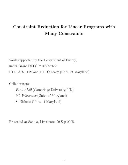
<strong>Constraint</strong> <strong>Reduction</strong> <strong>for</strong> <strong>Linear</strong> <strong>Programs</strong> <strong>with</strong><br />
<strong>Many</strong> <strong>Constraint</strong>s<br />
Work supported by the Department of Energy,<br />
under Grant DEFG0204ER25655.<br />
P.I.s: A.L. Tits and D.P. O’Leary (Univ. of Maryland)<br />
Collaborators:<br />
P.A. Absil (Cambridge University, UK)<br />
W. Woessner (Univ. of Maryland)<br />
S. Nicholls (Univ. of Maryland)<br />
Presented at Sandia, Livermore, 29 Sep 2005.<br />
1
Consider the following linear program in dual standard <strong>for</strong>m<br />
max b T y subject to A T y ≤ c, (1)<br />
where A is m × n. Suppose n ≫ m.<br />
Observations:<br />
• Interior-Point (IP) methods use search directions whose computation involves<br />
all constraints at every iteration.<br />
• Normally, only a few constraints (no more than m under nondegeneracy<br />
assumptions) are active at the solution. The others are “redundant”.<br />
b<br />
Objective:<br />
• Compute IP search direction based on a reduced Newton-KKT system,<br />
by adaptively selecting a small subset of critical columns of A.<br />
Hope:<br />
– Significantly reduced cost per iteration.<br />
– No drastic increase in the number of iterations.<br />
– Preserve theoretical convergence properties.<br />
2
Outline<br />
1. Background<br />
• Some related work<br />
• Notation<br />
• Primal-dual framework<br />
• Operation count – Reduced Newton-KKT system<br />
2. Reduced, Dual-Feasible PD Affine Scaling: µ = 0<br />
• Algorithm statement<br />
• Observations<br />
• Numerical experiments: Matlab<br />
• Convergence properties<br />
3. Reduced Mehrotra-Predictor-Corrector<br />
• Algorithm statement<br />
• Numerical experiments: Matlab<br />
4. Invariance under Trans<strong>for</strong>mations?<br />
5. Concluding Remarks<br />
3
Background<br />
Some related work<br />
• “Indicators” (to identify early the zero components of primal solution<br />
x ∗ ): El-Bakry et al.[1994], Facchinei et al.[2000].<br />
• “Column generation”, “build-up”, “build-down”: Ye [1992], den Hertog<br />
et al.[1992, 1994, 1995], Goffin et al.[1994], Ye [1997], Luo et al.[1999].<br />
– Focus is on complexity analysis;<br />
– Good numerical results on discretized semi-infinite programming<br />
problems; but typically, many more than m columns of A are retained.<br />
Notation<br />
n := {1, . . .,n},<br />
A = [a 1 , . . .,a n ], e = [1, ..., 1] T ,<br />
Given Q ⊆ n,<br />
A Q := col[a i : i ∈ Q],<br />
X Q := diag(x i : i ∈ Q),<br />
x Q := [x i : i ∈ Q] T<br />
S Q := diag(s i : i ∈ Q). s Q := [s i : i ∈ Q] T<br />
4
Background (cont’d)<br />
Primal-dual framework<br />
Primal-dual LP pair in standard <strong>for</strong>m:<br />
min c T x subject to Ax = b, x ≥ 0<br />
max b T y subject to A T y + s = c, s ≥ 0. (2)<br />
Perturbed (µ ≥ 0) KKT conditions of optimality:<br />
A T y + s − c = 0 (3)<br />
Ax − b = 0 (4)<br />
XSe = µe (5)<br />
x, s ≥ 0, (6)<br />
Given µ ≥ 0, µ-perturbed Newton-KKT system:<br />
⎡ ⎤ ⎡ ⎤ ⎡ ⎤<br />
0 A T I ∆x −r c<br />
⎢<br />
⎣A 0 0 ⎥ ⎢<br />
⎦ ⎣∆y⎥<br />
⎦ = ⎢<br />
⎣ −r b<br />
⎥<br />
⎦<br />
S 0 X ∆s −Xs + µe,<br />
<strong>with</strong> r b := Ax − b (primal residue) and r c := A T y + s − c (dual residue).<br />
5
Background (cont’d)<br />
Primal-dual framework (cont’d)<br />
Equivalently, (∆x, ∆y, ∆s) satisfy the normal equations:<br />
AS −1 XA T ∆y = −r b + A(−S −1 Xr c + x − µS −1 e)<br />
∆s = −A T ∆y − r c<br />
∆x = −x + µS −1 e − S −1 X∆s<br />
Simple interior-point iteration: Given x > 0, s > 0, y,<br />
• Select a value <strong>for</strong> µ (≥ 0);<br />
• Solve Newton-KKT system <strong>for</strong> ∆x, ∆y, ∆s;<br />
• Set x + := x + α P ∆x > 0, s + := s + α D ∆s > 0, y + := y + α D ∆y <strong>with</strong><br />
appropriate α P , α D (possibly <strong>for</strong>ced to be equal).<br />
Note: If (y, s) is dual feasible, then (y + , s + ) also is.<br />
6
Background (cont’d)<br />
Operation count – Reduced Newton-KKT system<br />
• Operation count (<strong>for</strong> a dense problem):<br />
- Forming H := AS −1 XA T : m 2 n;<br />
- Forming v := r b + A(x − S −1 (Xr c + µe)); 2mn;<br />
- Solving H∆y = v: m 3 /3 (Cholesky);<br />
- Computing ∆s = −A T ∆y − r c : 2mn;<br />
- Computing ∆x = −x + S −1 (−X∆s + µe): 2n;<br />
• Benefit in replacing A <strong>with</strong> A Q : n replaced <strong>with</strong> |Q|<br />
• Assume n ≫ m and m ≫ 1. Then main gain can be achieved in line 1,<br />
i.e., by merely replacing H <strong>with</strong> H Q := A Q S −1<br />
Q X QA T Q , and leaving the<br />
rest unchanged. This is done in the sequel.<br />
∗ Key question: How to select Q <strong>for</strong><br />
– Significantly reducing the work per iteration (|Q| small);<br />
– Avoiding a dramatic increase in number of iterations;<br />
– Preserving theoretical convergence properties.<br />
7
Reduced, Dual-Feasible PD Affine Scaling: µ = 0<br />
Algorithm statement<br />
Iteration rPDAS.<br />
Parameters. β ∈ (0, 1), x max > 0, x > 0, M ≥ m.<br />
Data. y, <strong>with</strong> A T y < c; s := c − A T y (> 0) (i.e., r c = 0); x > 0;<br />
Q ⊆ n, including the indices of M smallest entries of s.<br />
Step 1. Compute search direction.<br />
Step 2. Updates.<br />
Solve<br />
and compute<br />
A Q S −1<br />
Q X QA T Q ∆y = b<br />
∆s ← −A T ∆y<br />
˜x ← −S −1 X∆s<br />
(i) Primal update (appropriately clip the components of ˜x). Set<br />
x + i ← min{max{min{‖∆y‖ 2 + ‖˜x − ‖ 2 , x}, ˜x i }, x max }, ∀i ∈ n, (8)<br />
where (˜x − ) i := min{˜x i , 0}.<br />
(ii) Dual update (step along ∆y). Set<br />
⎧<br />
⎨<br />
∞ if ∆s i ≥ 0 ∀i ∈ n,<br />
t D ←<br />
⎩ min{(−s i /∆s i ) : ∆s i < 0, i ∈ n} otherwise.<br />
(9)<br />
Set ˆt D ← min{max{βt D , t D −‖∆y‖}, 1}.<br />
Set y + ← y + ˆt D ∆y, s + ← s + ˆt D ∆s. (So r c remains at 0.)<br />
8
Reduced, Dual-Feasible PD Affine Scaling: µ = 0<br />
Observations<br />
• (∆x Q , ∆y, ∆s Q ) constructed by iteration rPDAS, also satisfy<br />
∆s Q = −A T Q ∆y<br />
∆x Q = −x Q − S −1<br />
Q X Q∆s Q ,<br />
(10a)<br />
(10b)<br />
i.e., they satisfy the full set of normal equations associated <strong>with</strong> the<br />
constraint-reduced system. Equivalently, they satisfy the Newton system<br />
(<strong>with</strong> µ = 0 and r c = 0)<br />
⎡ ⎤⎡<br />
⎤ ⎡ ⎤<br />
0 A T Q I ∆x Q 0<br />
⎢<br />
⎣A Q 0 0 ⎥⎢<br />
⎦⎣<br />
∆y ⎥<br />
⎦ = ⎢<br />
⎣b − A Q x Q<br />
⎥<br />
⎦ .<br />
S Q 0 X Q ∆s Q −X Q s Q<br />
(This is a key ingredient to the local convergence analysis.)<br />
• Update rule (8), in particular the lower bound ‖∆y‖ 2 + ‖˜x − ‖ 2 , is instrumental<br />
to our convergence analysis. (As step along ∆x would not always<br />
allow such lower bound.)<br />
9
Reduced, Dual-Feasible PD Affine Scaling: µ = 0<br />
Numerical experiments: Matlab<br />
Heuristic used <strong>for</strong> Q: For given M ≥ m,<br />
Q = indexes of M smallest components of s.<br />
Parameter value: β = .99, x = 10 −5 , x max = 10 15 .<br />
Selection of x 0 : Based on Mehrotra’s [SIOPT, 1992] scheme.<br />
Test problems (<strong>with</strong> dual-feasible initial point)<br />
• Polytopic approximation of unit sphere (Semi-infinite problem)<br />
– entries of b ∼ N(0, 1);<br />
– columns of A uni<strong>for</strong>mly distributed on the unit sphere;<br />
– c = e, y 0 = 0;<br />
– m = 50, n = 20, 000.<br />
• “Fully random” problem<br />
– entries of A and b ∼ N(0, 1);<br />
– components of y 0 and s 0 uni<strong>for</strong>mly distributed on (0,1);<br />
– c = A T y 0 + s 0 to ensure dual feasibility;<br />
– m = 50, n = 20, 000.<br />
• SCSD1 (m = 77, n = 760) and SCSD6 (m = 147, n = 1350) from<br />
Netlib.<br />
10
Reduced, Dual-Feasible PD Affine Scaling: µ = 0<br />
Numerical experiments: Matlab (cont’d)<br />
The points on the plots correspond to different runs of Algorithm rPDAS<br />
on the same problem. The runs only differ by the number M of constraints<br />
that are retained in Q; this in<strong>for</strong>mation is indicated on the horizontal axis<br />
in relative value. The rightmost point thus corresponds to the experiment<br />
<strong>with</strong>out constraint reduction, while the points on the far left correspond to<br />
the most drastic constraint reduction.<br />
Observations:<br />
• In most cases, surprisingly, the number of iterations does NOT increase<br />
as M is reduced. Thus any gain in CPU per iteration directly translates<br />
into the same relative gain in overall CPU.<br />
• Displayed CPU values are purely indicative. Indeed, they will strongly depend<br />
on the implementation (in particular, how the product A Q S −1<br />
Q X QA T Q<br />
is computed), and on the possible sparsity of the data.<br />
• The algorithm sometimes fails <strong>for</strong> small |Q|. This is due to A Q losing<br />
rank, and accordingly A Q SQ −1X<br />
QA T Q<br />
becoming singular. (Note that this<br />
will almost surely not happen when A is generated randomly.) Schemes<br />
to bypass this difficulty are being investigated.<br />
11
80<br />
Number of iterations<br />
60<br />
40<br />
20<br />
0<br />
0 0.1 0.2 0.3 0.4 0.5 0.6 0.7 0.8 0.9 1<br />
CPU time (sec.)<br />
8<br />
6<br />
4<br />
2<br />
total<br />
<strong>for</strong>m H Q<br />
solves<br />
0<br />
0 0.1 0.2 0.3 0.4 0.5 0.6 0.7 0.8 0.9 1<br />
|Q|/n<br />
rPDAS on Polytopic approximation of unit sphere; m = 50, n = 20, 000.<br />
100<br />
Number of iterations<br />
80<br />
60<br />
40<br />
20<br />
0<br />
0 0.1 0.2 0.3 0.4 0.5 0.6 0.7 0.8 0.9 1<br />
CPU time (sec.)<br />
15<br />
10<br />
5<br />
total<br />
<strong>for</strong>m H Q<br />
solves<br />
0<br />
0 0.1 0.2 0.3 0.4 0.5 0.6 0.7 0.8 0.9 1<br />
|Q|/n<br />
rPDAS on “Fully random”; m = 50, n = 20, 000.<br />
12
40<br />
Number of iterations<br />
30<br />
20<br />
10<br />
0<br />
0 0.1 0.2 0.3 0.4 0.5 0.6 0.7 0.8 0.9 1<br />
CPU time (sec.)<br />
0.2<br />
0.15<br />
0.1<br />
0.05<br />
total<br />
<strong>for</strong>m H Q<br />
solves<br />
0<br />
0 0.1 0.2 0.3 0.4 0.5 0.6 0.7 0.8 0.9 1<br />
|Q|/n<br />
rPDAS on SCSD1: m = 77, n = 760.<br />
80<br />
Number of iterations<br />
60<br />
40<br />
20<br />
0<br />
0 0.1 0.2 0.3 0.4 0.5 0.6 0.7 0.8 0.9 1<br />
CPU time (sec.)<br />
0.5<br />
0.4<br />
0.3<br />
0.2<br />
0.1<br />
total<br />
<strong>for</strong>m H Q<br />
solves<br />
0<br />
0 0.1 0.2 0.3 0.4 0.5 0.6 0.7 0.8 0.9 1<br />
|Q|/n<br />
rPDAS on SCSD6: m = 147, n = 1350.<br />
13
Reduced, Dual-Feasible PD Affine Scaling: µ = 0<br />
Convergence properties<br />
Let F := {y : A T y ≤ c}. For y ∈ F, let I(y) := {i : a T i y = c i}.<br />
Assumption 1. All m × M submatrices of A have full (row) rank.<br />
Assumption 2. The dual (y) solution set is nonempty and bounded.<br />
Assumption 3. For all y ∈ F, the set {a i : i ∈ I(y)} is linear independent.<br />
Theorem. {y k } converges to the dual solution set.<br />
Assumption 4. The dual solution set is a singleton, say, {y ∗ }, and the<br />
associated KKT multiplier x ∗ satisfies x ∗ i < x max <strong>for</strong> all i.<br />
Theorem. {(x k , y k )} converges to (x ∗ , y ∗ ) Q-quadratically.<br />
• The global convergence analysis focuses on the monotone increase of the<br />
dual objective function b T y.<br />
• The lower bound ‖∆y‖ 2 + ‖˜x − ‖ 2 in the primal update <strong>for</strong>mula (8) is essential<br />
as it keeps the Newton-KKT matrix away from singularity as long<br />
as KKT points are not approached. (A step along the primal direction<br />
∆x would not allow <strong>for</strong> this.)<br />
14
Reduced Mehrotra-Predictor-Corrector<br />
Algorithm statement<br />
Iteration rMPC.<br />
Parameters. β ∈ (0, 1), M ≥ m.<br />
Data. y ∈ R m , s > 0, x > 0; µ := x T s/n;<br />
Q ⊆ n, including the indices of M leftmost components of<br />
c − A T y.<br />
Step 1. Compute affine scaling step.<br />
Solve<br />
A Q S −1<br />
Q X QA T Q ∆y = −r b + A(−S −1 Xr c + x)<br />
and compute<br />
∆s ← −A T ∆y − r c<br />
∆x ← −x − S −1 X∆s<br />
t aff<br />
P ← arg max{t ∈ [0, 1] | x + t∆x ≥ 0}<br />
t aff<br />
D ← arg max{t ∈ [0, 1] | x + t∆s ≥ 0}<br />
Step 2. Compute centering parameter.<br />
µ aff ← (x + t aff<br />
P ∆x)T (s + t aff<br />
D ∆s)/n<br />
σ ← (µ aff /µ) 3<br />
Step 3. Compute centering/corrector direction.<br />
Solve A Q S −1<br />
Q X QA T Q∆y cc = −AS −1 (σµe − ∆X∆s)<br />
and compute ∆s cc ← −A T ∆y cc<br />
∆x cc ← S −1 (σµe − ∆X∆s) − S −1 X∆s cc<br />
15
Step 4. Compute MPC step.<br />
∆x mpc ← ∆x + ∆x cc<br />
∆y mpc ← ∆y + ∆y cc<br />
∆s mpc ← ∆s + ∆s cc<br />
t max<br />
P ← arg max{t ∈ [0, 1] | x + t∆x mpc ≥ 0}<br />
t max<br />
D ← arg max{t ∈ [0, 1] | s + t∆s mpc ≥ 0}<br />
t P<br />
← min{βt max<br />
P , 1}<br />
t D ← min{βt max<br />
D , 1}<br />
Step 5. Updates.<br />
x + ← x + t P ∆x mpc<br />
y + ← y + t D ∆y mpc<br />
s + ← s + t D ∆s mpc<br />
Numerical experiments <strong>with</strong> dual-feasible initial point<br />
Algorithm rMPC was run on the same problems as rPDAS, <strong>with</strong> the same<br />
(dual-feasible) initial points. The results are reported in the next few slides.<br />
16
50<br />
Number of iterations<br />
40<br />
30<br />
20<br />
10<br />
0<br />
0 0.1 0.2 0.3 0.4 0.5 0.6 0.7 0.8 0.9 1<br />
CPU time (sec.)<br />
10<br />
8<br />
6<br />
4<br />
2<br />
total<br />
<strong>for</strong>m H Q<br />
solves<br />
0<br />
0 0.1 0.2 0.3 0.4 0.5 0.6 0.7 0.8 0.9 1<br />
|Q|/n<br />
rMPC on Polytopic approx. of unit sphere, w/ dual-feasible init. pt; m = 50, n = 20, 000.<br />
40<br />
Number of iterations<br />
30<br />
20<br />
10<br />
0<br />
0 0.1 0.2 0.3 0.4 0.5 0.6 0.7 0.8 0.9 1<br />
CPU time (sec.)<br />
8<br />
6<br />
4<br />
2<br />
total<br />
<strong>for</strong>m H Q<br />
solves<br />
0<br />
0 0.1 0.2 0.3 0.4 0.5 0.6 0.7 0.8 0.9 1<br />
|Q|/n<br />
rMPC on “Fully random”, <strong>with</strong> dual-feasible initial point; m = 50, n = 20, 000.<br />
17
Number of iterations<br />
20<br />
15<br />
10<br />
5<br />
0<br />
0 0.1 0.2 0.3 0.4 0.5 0.6 0.7 0.8 0.9 1<br />
CPU time (sec.)<br />
0.2<br />
0.15<br />
0.1<br />
0.05<br />
total<br />
<strong>for</strong>m H Q<br />
solves<br />
0<br />
0 0.1 0.2 0.3 0.4 0.5 0.6 0.7 0.8 0.9 1<br />
|Q|/n<br />
rMPC on SCSD1, <strong>with</strong> dual-feasible initial point: m = 77, n = 760.<br />
Number of iterations<br />
35<br />
30<br />
25<br />
20<br />
15<br />
10<br />
5<br />
0<br />
0 0.1 0.2 0.3 0.4 0.5 0.6 0.7 0.8 0.9 1<br />
CPU time (sec.)<br />
0.4<br />
0.3<br />
0.2<br />
0.1<br />
total<br />
<strong>for</strong>m H Q<br />
solves<br />
0<br />
0 0.1 0.2 0.3 0.4 0.5 0.6 0.7 0.8 0.9 1<br />
|Q|/n<br />
rMPC on SCSD6, <strong>with</strong> dual-feasible initial point: m = 147, n = 1350.<br />
18
Reduced Mehrotra-Predictor-Corrector (cont’d)<br />
Numerical experiments <strong>with</strong> infeasible initial point<br />
The next few slides report results obtained on the same problem, but <strong>with</strong><br />
the (usually infeasible) initial point as recommended by Mehrotra [SIOPT,<br />
1992].<br />
19
Number of iterations<br />
70<br />
60<br />
50<br />
40<br />
30<br />
20<br />
10<br />
0<br />
0 0.1 0.2 0.3 0.4 0.5 0.6 0.7 0.8 0.9 1<br />
CPU time (sec.)<br />
8<br />
6<br />
4<br />
2<br />
total<br />
<strong>for</strong>m H Q<br />
solves<br />
0<br />
0 0.1 0.2 0.3 0.4 0.5 0.6 0.7 0.8 0.9 1<br />
|Q|/n<br />
rMPC on Polytopic approx. of unit sphere, w/ infeasible init. pt; m = 50, n = 20, 000.<br />
80<br />
Number of iterations<br />
60<br />
40<br />
20<br />
0<br />
0 0.1 0.2 0.3 0.4 0.5 0.6 0.7 0.8 0.9 1<br />
CPU time (sec.)<br />
15<br />
10<br />
5<br />
total<br />
<strong>for</strong>m H Q<br />
solves<br />
0<br />
0 0.1 0.2 0.3 0.4 0.5 0.6 0.7 0.8 0.9 1<br />
|Q|/n<br />
rMPC on “Fully random”, <strong>with</strong> infeasible initial point: m = 50, n = 20, 000.<br />
20
40<br />
Number of iterations<br />
30<br />
20<br />
10<br />
0<br />
0 0.1 0.2 0.3 0.4 0.5 0.6 0.7 0.8 0.9 1<br />
CPU time (sec.)<br />
0.25<br />
0.2<br />
0.15<br />
0.1<br />
0.05<br />
total<br />
<strong>for</strong>m H Q<br />
solves<br />
0<br />
0 0.1 0.2 0.3 0.4 0.5 0.6 0.7 0.8 0.9 1<br />
|Q|/n<br />
rMPC on SCSD1, <strong>with</strong> infeasible initial point: m = 77, n = 760.<br />
50<br />
Number of iterations<br />
40<br />
30<br />
20<br />
10<br />
0<br />
0 0.1 0.2 0.3 0.4 0.5 0.6 0.7 0.8 0.9 1<br />
CPU time (sec.)<br />
0.8<br />
0.6<br />
0.4<br />
0.2<br />
total<br />
<strong>for</strong>m H Q<br />
solves<br />
0<br />
0 0.1 0.2 0.3 0.4 0.5 0.6 0.7 0.8 0.9 1<br />
|Q|/n<br />
rMPC on SCSD6, <strong>with</strong> infeasible initial point: m = 147, n = 1350.<br />
21
Invariance under Trans<strong>for</strong>mations?<br />
Let P ∈ R m×m , nonsingular; v ∈ R m ; R ∈ R n×n > 0, diagonal. 1<br />
Consider the trans<strong>for</strong>mation<br />
x ← R −1 x; s ← Rs; y ← P −T y + v.<br />
(Also, A ← PAR; b ← Pb; c ← Rc + RA T P T v.)<br />
• MPC: (P, v, R)-invariant.<br />
• rMPC: (P, v)-invariant.<br />
– R-invariance is affected by the rule <strong>for</strong> selection of Q.<br />
– It can be recovered by substituting (c i −a T i y)/(c i−a T i y0 ) <strong>for</strong> (c i −a T i y).<br />
• PDAS: (P, v)-invariant <strong>with</strong> orthogonal P, i.e., invariant under Euclidean<br />
trans<strong>for</strong>mations of the dual space. (Not general P: due to use of<br />
‖∆y‖. Not R: due to use of ‖˜x − ‖, x, and x max .)<br />
– Nonsingular diagonal P can be allowed by replacing ‖∆y‖ <strong>with</strong><br />
‖(∆Y 0 ) −1 ∆y‖;.<br />
– Scalar×orthogonal P can be allowed by replacing ‖∆y‖ <strong>with</strong> ‖∆y‖/‖∆y 0 ‖.<br />
– R-invariance recovered by replacing ‖˜x − ‖ <strong>with</strong> ‖(∆X 0 ) −1˜x − ‖, and<br />
similarly <strong>for</strong> the fixed bounds.<br />
• rPDAS: R-invariance can be recovered as in rMPC.<br />
1 R must be thus restricted in order <strong>for</strong> x ≥ 0 to be preserved.<br />
22
Concluding Remarks<br />
“Reduced” version of an primal-dual affine scaling algorithm (rPDAS) and<br />
of Mehrotra’s predictor-corrector algorithm (rMPC) were proposed.<br />
• When n ≫ m and m ≫ 1, <strong>for</strong> both rPDAS and rMPC, major reduction<br />
in CPU per iteration can be achieved.<br />
• Under nondegeneracy assumptions, rPDAS is proved to converge quadratically<br />
in the primal-dual space; a convergence proof <strong>for</strong> rMPC is lacking<br />
at this time.<br />
• Numerical experiments show that<br />
– The number of iterations to convergence remains essentially constant<br />
as |Q| decreases, down to a small multiple of m.<br />
– On some problems (e.g., SCSD1, SCSD6), when |Q| is reduced below<br />
a certain value, the algorithm fails due to A Q losing rank. Schemes<br />
to bypass this difficulty are being investigated.<br />
This presentation can be downloaded from<br />
http://www.isr.umd.edu/~andre/sandia050929.pdf<br />
and the full paper and Matlab script from<br />
http://www.csit.fsu.edu/~absil/Publi/reducedLP.htm<br />
23