Tutorial Modeling of monolith reactors

Introduction to Monolith
Reactor Modelling:
Mass, Energy and Momentum Transport
R.E. Hayes
Department of Chemical and Materials
Engineering, University of Alberta,
Edmonton, Alberta, Canada
MODEGAT 14-15 September 2009
1

Objectives of this presentation
• To give an introductory overview to the
area of monolith reactor modelling
• To high light some of the factors that
must be taken into consideration when
choosing a model.
2

Why use computer modelling?
• Experiments are expensive and take time.
• Analysis of reactors can be difficult, especially for
fast highly exothermic reactions. Non-intrusive
measurement methods may not be available.
• Modelling can eliminate scenarios that do not
offer promise.
• Faster design and optimisation.
Models are not intended to eliminate experiments completely.
3

Typical catalytic converter
•The The catalytic converter uses a metal or ceramic monolith
support structure.
•Typical Typical automotive converters use 400 CPSI cell density
Hayes and Kolaczkowski, Chem.
Eng. Sci., 49, 3587, 1994.
Heck and Farrauto, Catalytic Air
Pollution Control, 2002
4

Observations
• The problem involves the transport of mass, energy
and momentum. It is a multi-physics
problem.
• Transport occurs at different scales in space.
• The transient response of the gas phase and solid
phase occurs at different time scales.
• Modelling of monolith reactors is thus an exercise in
multi-scale modelling.
The monolith reactor presents a challenging modelling problem.
5

Heterogeneous catalytic reactions
Heterogeneous gas phase catalytic reactions typically comprise the same steps.
Fluid flow over the solid results in a
boundary layer through which heat and
mass diffuse to the gas/solid interface.
Reactants diffuse into the porous
catalyst.
External
catalyst
surface
catalyst
pore
Bulk gas
Reactants adsorb on the active sites.
The reaction occurs on the active sites,
located on the walls of the tortuous pores.
Products desorb and diffuse back to the
surface, and then through the boundary
layer to the bulk fluid.
6

Model Scales
Micro scale: At the atomic/molecular level, the basic chemistry
involves a set of adsorption/desorption and surface reaction
steps. The genuine mechanism may be very complicated.
Gas Phase
Catalyst
Meso scale: Single channel of a monolith. Includes gas
phase flow, transport to the surface of the washcoat by
diffusion, diffusion and reaction in the washcoat. The
basic process in a heterogeneous catalytic reaction are
present at the meso scale.
Macro scale: Entire catalytic converter, which
includes transport and interaction among channels.
7

Model complexity: Points to note
• How much complexity is wanted and or needed?
– At what level do you wish to model?
– How much information do you want to include?
– Do you need to include all of the scales?
• The model should be as simple as possible, but not
simpler (Albert Einstein).
• Models do not have to be perfect to be useful.
Gas Phase
Catalyst
8

Mathematical formulation
• The fundamental model is represented by a set of
equations, which include key assumptions
– Algebraic equations, linear or non-linear
– Ordinary differential equations (IVP or BVP)
– Partial differential equations
• Practical monolith modelling problems do not have
analytical solutions; models are solved numerically.
• The model selected and the way it is represented will
determine the numerical method used for its solution.
9

Mathematical formulation
• Reactors are fundamentally distributed parameter
systems ; Concentration, temperature and velocity
vary with spatial coordinate.
• The dimensionality (and hence complexity) can be
reduced by using average parameter values over
specified model dimensions. The result is referred
to as a lumped parameter model.
• Lumped parameter models are approximations.
10

Basic models in common use
• Single channel of monolith structure
– 1D, 2D or 3D
– Diffusion in the washcoat may be considered
• Whole reactor with variable channel conditions
and channel interactions
– 2D or 3D , several model options exist
– The upstream and downstream duct work might
be included
11

Single channel model (SCM)
• Single channel of monolith structure
• For a radially uniform monolith, the SCM is
representative of the whole reactor
• There are many approaches to writing a single
channel model:
– PDE models (all 2D and 3D models, some 1D)
– ODE models (some 1D models)
– Algebraic equations only (some 1D models)
12

The 3D SCM
• The real monolith does not have
axial symmetry.
• The washcoat can have a variety
of possible shapes.
• 3D is required for exact channel
representation
13

The 3D SCM
• A minimum of a one-eighth
section must be considered.
• For complex shapes such as the
“sinusoidal” channel, the entire
cross section must be
considered.
• There is no analytical solution
for the velocity.
• Must solve the transport
equations in three dimensions.
14

The 2D approximate SCM
• The 2D model approximates the
channel as a right circular cylinder
with a uniform annular washcoat
layer, thus giving axi-symmetry.
• The flow area, washcoat area and
substrate area should be the same
for each system.
• The 2D model is still the most
complex model that is used
routinely.
• The fully developed flow field can
be approximated, thus reducing the
number of equations to solve.
15

2D and 3D SCM
• 2D and 3D SCM are both distributed parameter
models.
• Temperature, concentrations and velocities vary with
both axial (flow direction) and radial (transverse to
flow) directions.
• The most general model requires the solution of a set
of coupled non-linear partial differential equations.
• The equations are the same in each case – only the
number of space dimensions changes.
16

The 2D SCM
• All of the physical/chemical processes present
in 2D and 3D can be illustrated using a two
dimensional model.
Mass Transfer
Direction of flow
Heat Transfer
Convection Radiation
washcoat Diffusion and reaction Conduction
substrate
Conduction
Centreline of wall
17

Basic solution procedure
• Each physical space (fluid, washcoat and substrate)
is a computational domain governed by the
conservation equations.
• Write the governing differential equations for each
domain (fluid, washcoat and substrate)
• Often only the solid state energy balance equations
retain the transient terms, owing to the relative
magnitude of the time scales for fluid and solid.
18

Modelling the fluid domain
Velocity and pressure are obtained from the Navier-Stokes equation
and the equation of continuity:
⎡
( ) (
T
( ) )
⎛2η
⎞ ⎤
ρ vi∇ v = ∇i⎢− pI + η ∇ v + ∇v − ⎜ −κ ( ∇ v)
I
3
⎟ i ⎥
⎣
⎝ ⎠ ⎦
( v) 0
∇i
ρ =
The density depends on temperature.
The mass balance (assuming Fick’s law) is:
( D w ) v ( w ) 0
∇⋅ ρ ∇ − ρ⋅∇ =
A A A
The energy balance is:
( k T) ( C ) vi
T 0
∇i
∇ − ρ ∇ =
f p f
Species conservation should be
expressed in terms of the mass
fraction because mass is conserved.
19

Observations
• The fluid equations are very classical and can be
readily solved.
• The mass and energy balances are coupled to the
washcoat at the gas solid interface.
• A zero slip condition is usually imposed at the gas
solid interface and a zero velocity boundary
condition imposed.
• One mass balance equation needed for each
species.
20

Modelling the washcoat domain
• The washcoat is a porous matrix containing solid
and fluid fractions.
• The diffusion/reaction occurs in the fluid fraction,
which is comprised of a network of tortuous pores.
• It is too complicated to model the actual diffusion
in the porous network (and the structure is
unknown in any case)
• Diffusion is thus assumed to occur across the entire
matrix and is governed by an effective diffusion
coefficient, with a Fickian type of approach.
21

Washcoat balance equations:
The mass balance equations are solved for the washcoat:
( )
∇⋅ ( D ) ρ ∇w − ( − R ) = 0
eff A A A
One mass balance for each species
The energy balance is:
∂T
R p S
( k ) ( ) ( )
eff T H ( RA
) C
∇i
∇ + −Δ − = ρ
∂t
Normally the momentum balance equation is not solved in the washcoat.
22

Diffusion in the washcoat
• Diffusion in the pore is governed by a combination
of bulk diffusion (molecular collisions) and Knudsen
diffusion (collisions of molecules with the wall).
• The relative importance of the two depends on the
gas pressure and the pore size.
• The effective diffusion coefficient is then computed
by adjusting for catalyst porosity and tortuosity.
• For a real catalyst with a given pore size
distribution, the calculation of effective diffusion
coefficients is not obvious.
23

Diffusion in the washcoat
• For binary eqi-molar counter diffusion of molecules
A and B we write, for the diffusion of A:
D
0.5
⎛ 1 1 ⎞
0.01013⎜
+
M M
⎟
⎝ ⎠ T
P
A B
AB =
0.333 0.333
(( ∑ ) ( ) )
νi
+ ∑νi
A
Bulk diffusion: Fuller correlation
1 1 1
= +
( Dpore) D ( D )
A
AB
Diffusion coefficient in the pore
K
B
A
1.75
( D K ) A
= 48.5 d p
M A
Knudsen diffusion
( D ) = ( D pore )
Effective diffusion coefficient
in the washcoat
T
eff A A
ε
τ
24

Modelling the substrate domain
The energy balance is:
∂ T
eff p S
( k T) ( C )
∇i
∇ = ρ
∂ t
The substrate is a porous medium and is modelled using effective properties.
25

Remarks: 2D and 3D models
• The basic equations are the same for 2D and 3D
models.
• Solution can be done using commercial or custom
software 3D models will take much longer to solve.
• Normally, a finite element or finite volume method
will be used.
• For steady state models the substrate equations
can be eliminated.
26

Comparing 2D and 3D models
• The channel reconfiguration can cause model
differences.
Increasing boundary
temperature
Reactant concentration at two temperatures in a washcoat fillet.
27

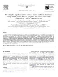
Comparing 2D and 3D models
Reactant concentration in a complex shape
28

Comparing 2D and 3D models
• The following light-off simulations show some
comparisons between 2D and 3D models.
• 2D model uses a circular washcoat and a
circular substrate (circle/circle)
• 3D model 1 uses a circular washcoat in a
square substrate (circle/square)
• 3D model 2 uses a square washcoat in a
square substrate (square/square).
More et al., Topics in Catalysis, 37 155 (2006)
29

Comparing 2D and 3D models
100
100
80
Circle/circle
Circle/square
Square/square
80
Circle/circle
Circle/square
Square/square
Percentage Conversion
60
40
Percentage Conversion
60
40
20
20
0
475 500 525 550
Inlet Gas Temperature /K
0
475 500 525 550 575
Inlet Gas Temperature /K
Inlet temperature ramp rate of 30 K/min at a GHSV of 20 000 h -1 and 80 000 h -1 .
More et al., Topics in Catalysis, 37 155 (2006)
30

Comparing 2D and 3D models
Percentage Conversion
100
80
60
40
20
Circle/circle
Circle/square
Square/square
0
500 520 540 560 580 600 620 640
Inlet temperature / K
Inlet temperature ramp rate of 300 K/min at a GHSV of 80 000 h -1 .
More et al., Topics in Catalysis, 37 155 (2006)
31

The 1D SCM approximation
• 2D and 3D models can be time consuming to run
and may not be necessary.
• The radial dimension is eliminated using radial
average properties. The model is transformed into a
lumped parameter model in the radial direction.
• Parameter lumping introduces a discontinuity at the
gas solid interface which is handled using mass and
heat transfer coefficients.
• The washcoat and substrate are collapsed into a
single one dimensional equation.
32

Review of boundary layer flow
Flow over a flat plate with exothermic
U ∞
reaction at the surface:
δ
Boundary layers develop for velocity,
temperature and concentration.
T ∞
δ T
T S
C C∞ ∞
C S
U ∞
T ∞
δ C
The boundary layer thickness increases with
length
The boundary layers have different thickness:
δ n δ n δ
= Sc = Pr
T
=
δ δ δ
C T C
Sc
Pr
n
n
33

Thermal boundary layer
T ∞
T ∞
T S
δ T
The heat transfer at the surface is :
The heat transfer can be defined as:
∂T
q′′ = −k
∂
y
y = 0
( )
′′ = −
q h TS
T ∞
The heat transfer coefficient h assumes a value to make the equality true.
If the temperature gradient at the surface is known, then h can be calculated.
34

Boundary layers in a tube
• At the entrance, boundary
layers grow from the surface.
• After the entry length, the
boundary layers meet.
• The fully developed region can
be considered a boundary
layer flow.
With reaction at the wall, the concentration
boundary layer development is similar.
• For laminar flow in a tube, the
velocity, temperature and
concentration fields can be
obtained from the solution of
the governing PDE.
35

Heat transfer in a tube
• In a tube, the flow becomes fully developed after
an entry length.
• There is no well defined reference temperature
external to the boundary layer, and therefore the
heat transfer coefficient is defined in terms of the
mixing cup temperatures (average radial
temperature)
• The mass transfer coefficient is defined in a
similar way.
36

Heat and mass transfer
• Heat and mass transfer coefficients can be
expressed in terms of dimensionless groups, the
Nusselt and Sherwood numbers.
• For a circular tube:
hD
k
=
Nu
km
D
D
A
=
Sh
• The heat and mass transfer coefficients can be
calculated by solving the 2D or 3D flow problems.
37

1D SCM: Model equations
• The form of the equation depends on the channel
geometry and the basis for the reaction rate:
• Example is shown for a circular tube with the rate
expressed in terms of washcoat volume:
38

1D SCM mass balances
The fluid phase mass balance expressed in terms of the mixing
cup concentration and the mass transfer coefficient is:
∂ ⎛ ∂wA, f ⎞ ∂wA,
f
⎛ 4 ⎞
⎜DAρf ⎟ − ( ρ f v) i − kmρf ( wA, f − wA,
S)
⎜ ⎟ =
∂z ⎝ ∂z ⎠ ∂z ⎝ DH
⎠
0
The axial diffusion coefficient is now a dispersion coefficient.
The velocity is an average velocity.
39

1D SCM mass balances
The solid phase mass balance is:
4 D
2 2
( D − D )
WC
( ) A, − A, = η(
− A )
k ρ w w R
m f f S S
Washcoat diffusion is included via the effectiveness factor.
The rate here is evaluated at the surface temperature and
concentration.
The rate is expressed in terms of washcoat volume.
40

1D SCM energy balances
The fluid phase energy balance is:
d ⎛ dTf
dTf
4
⎜k ⎞ I ⎟ − vm ( ρ Cp
) + h
f
( TS − Tf
) =
dz⎝
dz ⎠
d z D
0
The fluid thermal conductivity is an effective value that accounts for laminar flow.
The solid phase energy balance is:
∂ ⎛
⎛ ⎞
⎜k ⎟ h T T H R C
∂z⎝ ∂z ⎠
⎜ ⎟
⎝ ⎠
∂t
2 2
∂TS ⎞ 4 D
DWC − D ∂TS
S − ( ) ( ) ( A ) ( )
2 2 S − f − η Δ R ⎜
2 2
⎟ − = ρ
S P S
( DS
− D )
DS
− D
The solid thermal conductivity is an average value for washcoat and substrate.
41

Nusselt and Sherwood numbers
• The correct values of Nu and Sh are not obvious.
• In the fully developed region, the heat and mass
transfer coefficients are constant. The value
depends on the wall boundary condition.
• The classical boundary conditions are constant wall
temperature and constant wall flux.
• With a reaction on the surface, neither boundary
condition is true.
42

Nusselt and Sherwood numbers
• For flow in a circular tube with constant physical
properties, the classical result is:
43

Nusselt and Sherwood numbers
• Equations for the local Nu for Pr=0.7 with combined
entry length have been proposed. They can be
expressed generically as:
⎡
⎛ 50
Nu = C1 × ⎢ 1+ C2
Gz exp ⎜ −
⎣
⎝ Gz
⎞⎤
⎟⎥
⎠⎦
The constants depend on channel
shape and wall boundary condition
The value with reaction is found by interpolation between the values for
constant wall temperature and constant wall flux.:
Nu
2
H
⎛ NuH
⎞
Nu = Nu − Da + ⎜Nu − Da ⎟ + 4Da Nu
NuT
⎝ NuT
⎠
H H H
2
44

Nusselt and Sherwood numbers
• However, when the properties are not constant, the
entry length can be more complicated:
Nu
7
6
5
T = 500 K
T = 450 K
T = 550 K
Local Nusselt number
obtained from entry length
solutions for laminar flow in a
channel with different wall
temperature. No reaction.
4
More, MSc Thesis, University
of Alberta, 2007
3
0.001 0.01 0.1 1
1/Gz
45

Nusselt and Sherwood numbers
• So, what should we choose for the correct value?
• On the bright side, for circular channels, it might not be
that important:
100
Percentage Conversion
80
60
40
20
Nu = 4
Nu = 3
Nu = 5
Nu = 30
Axial conversion for a
typical monolith channel for
CO oxidation.
More, MSc Thesis,
University of Alberta, 2007
0
0.00 0.02 0.04 0.06 0.08 0.10
Axial Distance, m
46

Nusselt and Sherwood numbers
• However, for non-circular channels,
or non-uniform washcoat, the Nu and
Sh can vary around the washcoat
perimeter.
(a)
Sherwood number
6
5
4
3
2
550K
600K
650K
700K
750K
800K
850K
900K
Sherwood number along the
washcoat/channel interface
for the case of a circular
channel in a square
substrate. Interface length
shown corresponds to 1/8th
of the total interface. Fully
developed flow.
1
0 50 100 150 200 250 300 350 400
Distance along the interface, microns
Hayes et al. Chem. Eng. Sci., 59
3169 (2004).
47

Comparing 1D and 2D models
• 1D models can give very close agreement to
2D models in many situations.
• Generally the most difficult region to map
exactly will be the developing flow region, but
that length is often not significant.
Several studies in the literature comparing 1D and 2D models,
e.g. Groppi and Tronconi, Aiche Journal 1996.
48

Simplified 1D models
• Dispersion in the gas phase is sometimes ignored,
and plug flow assumed.
• If axial conduction in the solid phase is ignored, the
model can be reduced to an initial value problem.
• With these two assumptions, the channel can be
modelled as a finite number of stirred tanks in
series.
49

The effectiveness factor
Because the washcoat thickness is not explicitly
modelled, the washcoat diffusion is incorporated
using an effectiveness factor, defined as:
η =
Average reaction rate in washcoat
Rate evaluated at surface conditions
The effectiveness factor can be estimated from a submodel
that usually involves solving a 1D diffusion-reaction
problem. Washcoat geometry effects may be included.
Hayes, et al Chemical Engineering Science, 62 2209-2215, 2007.
Hayes, et al Chemical Engineering Science, 59 3169-3181, 2004.
50

Models for the converter
• In reality the channels in the converter may not
all have the same operating conditions.
• The substrate constrains the velocity and
concentrations to each channel, but heat transfer
can occur among the channels.
• A model of the entire converter may therefore be
required. There are two general methods for
modelling a converter:
– Discrete models
– Continuum models
51

Discrete converter models
• In a discrete model both the fluid and solid
domains are solved:
End view of a quarter section of a circular
monolith with imposed temperature
gradient.
Heat transfer occurs through a combination
of gas and solid with very different
properties.
Hayes et al., Catalysis Today, 2009
52

Discrete converter models
• A passenger car converter has
about 7 – 10 thousand channels
• Laboratory tests often use 1-2” 1
diameter cores with 300 – 1200
channels
Discretizing the entire physical space result in a problem too large to solve
by conventional means. Until new methods are proven typically use ….
53

Continuum converter models
• Classical porous media models treat the domain as
a continuum containing fluid and solid phases.
• The common term for developing the resulting
equations is called volume averaging – the balances
are made on a representative elemental volume
that contains both fluid and solid
• Each node in the computational domain represents
both a fluid and a solid – the spatial identity is lost.
• The conservation equations are then fairly classical:
Zygourakis, K. (1989). Chemical Engineering Science, 44, 2075-2086.
54

Momentum balance equation
Velocity and pressure are obtained from the Volume Averaged Navier-
Stokes equation and the equation of continuity:
⎡
( ) (
T
( ) )
⎛2η
⎞ ⎤
ρ vi∇ v = ∇i⎢− pI + η ∇ v + ∇v − ⎜ −κ⎟( ∇ iv)
I + S i
3
⎥
⎣
⎝ ⎠ ⎦
( v) 0
∇i
ρ =
The velocity is the superficial velocity.
The source term S accounts for the porous inertia.
The Brinkman
equation is a classical
version of the VANS
⎛ μ 1
S i = − ⎜ v i + C2
ρ
2
f v
⎝ K
v i
⎞
⎟
⎠
K is the permeability.
For laminar flow, the second term is zero.
55

Energy and mass balances
• There are two main classes of porous media models.
• Heterogeneous model:
– The fluid and solid temperatures and concentrations
are taken to be different. The two phases are coupled
using heat and mass transfer coefficients.
• Pseudo-homogeneous model
– The fluid and solid temperatures and concentrations
are taken to be the same. This situation corresponds
to infinitely large heat and mass transfer coefficients.
For transient simulations the heterogeneous model is recommended.
56

Energy balances
The fluid phase energy balance is:
∂T
f
φρ f CPf , + ρ fCPf , v i ∇ Tf = ∇ i ( keff, f∇Tf)
− hav( Tf−TS)
∂ t
The solid phase energy balance is:
∂ T
S
( 1 −φ) ρ C = ∇i(
k ∇ T ) + ha ( T − T ) + ( ΔH ) η( R )
S P, S eff, S S v f S R i i
∂ t i = 1
m
∑
The effective thermal conductivity for each phase depends on the
porosity and material properties.
see Hayes et al., Catalysis Today 2009
57

Mass balances
The fluid phase mass balance is:
( f wif , ) fv wif , ( Dim , wif , ) kmav f( wif , wiS
, )
∂
φ ρ + ρ ∇ = ∇ φρ ∇ + ρ −
∂t
i i
( )
Mass diffusion occurs only in the flow direction
The solid phase mass balance is:
0 = η i Ri + kmavρf wi, f − wi,
S
Washcoat diffusion is included via the effectiveness factor
58

Continuum model
• In effect, the continuum model solves a set of 1D
single channel models with channel coupling via
solid phase heat transfer.
• However, every channel is not modelled.
• Heat and mass transfer coefficients are the same
as used in the 1D SCM.
• The continuum model consists of a set of coupled
PDE, which are solved using the FEM or the FVM.
59

Example:
3D reverse flow Condor TM converter
3D heterogeneous model. 10 litre converter
for methane IC engine with reverse flow.
Fluent was used, dual zone model.
Liu et al. Computers and Chemical Engineering, 31 292 (2007)
60

Model validation
• All models must be validated for:
– (1) Coding (errors in model implementation)
– (2) Numerical errors
– (3) Simplifying assumptions
• Models can be validated by
– Comparison to experiments
– Analytical solutions
• No model can be completely validated.
61

Model validation - Example
• Oxidation of methane in air
• Reactor wall temperature measured along reactor
length
• Step changes in methane concentration
• Kinetics determined in separate experiments
• 2D single channel model with washcoat diffusion
62

Model validation - Example
Heating curve with step increase
in methane concentration
Cooling curve when
methane switched off
Hayes et al, I&EC Research, 35 406 (1996)
63

Concluding remarks
• An appropriately chosen model can provide a
useful design aid.
• Models can be used as a tool to investigate the
phenomena occurring in the reactor.
• Recognize the limitations imposed by the
simplifying assumptions.
• Good values for the physical properties are
essential.
64

Advertising supplement
R.E. Hayes and S.T. Kolaczkowski
Introduction to Catalytic
Combustion
Taylor and Francis, 1997
65