Nonlinear stochastic differential equations and 1/f noise
Nonlinear stochastic differential equations and 1/f noise
Nonlinear stochastic differential equations and 1/f noise

You also want an ePaper? Increase the reach of your titles
YUMPU automatically turns print PDFs into web optimized ePapers that Google loves.
<strong>Nonlinear</strong> <strong>stochastic</strong> <strong>differential</strong> <strong>equations</strong><br />
<strong>and</strong> 1/f <strong>noise</strong><br />
Julius Ruseckas <strong>and</strong> Bronsilovas Kaulakys<br />
Institute of Theoretical Physics <strong>and</strong> Astronomy, Vilnius University, Lithuania<br />
August 28, 2012<br />
Julius Ruseckas (Lithuania) <strong>Nonlinear</strong> <strong>stochastic</strong> <strong>differential</strong> <strong>equations</strong> August 28, 2012 1 / 32
Outline<br />
1 Introduction: 1/f <strong>noise</strong><br />
2 Stochastic <strong>differential</strong> <strong>equations</strong> giving 1/f <strong>noise</strong><br />
3 Some models resulting in proposed SDE<br />
Point processes<br />
Simple model of herding behavior<br />
4 Summary<br />
Julius Ruseckas (Lithuania) <strong>Nonlinear</strong> <strong>stochastic</strong> <strong>differential</strong> <strong>equations</strong> August 28, 2012 2 / 32
What is 1/f <strong>noise</strong>?<br />
1/f <strong>noise</strong><br />
a type of <strong>noise</strong> whose power spectral density S(f ) behaves like<br />
S(f ) ∼ 1/f β , β is close to 1<br />
occasionally called “flicker <strong>noise</strong>”<br />
or “pink <strong>noise</strong>”<br />
Julius Ruseckas (Lithuania) <strong>Nonlinear</strong> <strong>stochastic</strong> <strong>differential</strong> <strong>equations</strong> August 28, 2012 3 / 32
1/f <strong>noise</strong><br />
First observed (in 1925) by Johnson in vacuum tubes.<br />
Julius Ruseckas (Lithuania) <strong>Nonlinear</strong> <strong>stochastic</strong> <strong>differential</strong> <strong>equations</strong> August 28, 2012 4 / 32
1/f <strong>noise</strong><br />
Fluctuations of signals exhibiting 1/f behavior of the power spectral<br />
density at low frequencies have been observed in a wide variety of<br />
physical, geophysical, biological, financial, traffic, Internet,<br />
astrophysical <strong>and</strong> other systems.<br />
Julius Ruseckas (Lithuania) <strong>Nonlinear</strong> <strong>stochastic</strong> <strong>differential</strong> <strong>equations</strong> August 28, 2012 5 / 32
1/f <strong>noise</strong><br />
Many mathematical models:<br />
Superposition of relaxation processes<br />
S(f ) =<br />
∫ γ2<br />
γ 1<br />
N πN<br />
γ 2 dγ ≈<br />
+ ω2 2ω , γ 1 ≪ ω ≪ γ 2<br />
Dynamical systems at the edge of chaos<br />
x n+1 = x n + x z n mod 1<br />
Alternating fractal renewal process<br />
Self-Organized Criticallity<br />
Julius Ruseckas (Lithuania) <strong>Nonlinear</strong> <strong>stochastic</strong> <strong>differential</strong> <strong>equations</strong> August 28, 2012 6 / 32
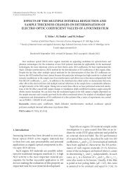
A bibliography on 1/f <strong>noise</strong> is vast<br />
Published items in each year. Topic: 1/f <strong>noise</strong>, 1/f fluctuations, flicker<br />
<strong>noise</strong>, pink <strong>noise</strong> (Web of Science)<br />
Julius Ruseckas (Lithuania) <strong>Nonlinear</strong> <strong>stochastic</strong> <strong>differential</strong> <strong>equations</strong> August 28, 2012 7 / 32
1/f <strong>noise</strong><br />
Goal<br />
1/f <strong>noise</strong> is intermediate between white <strong>noise</strong>, S(f ) ∼ 1/f 0 <strong>and</strong><br />
Brownian motion S(f ) ∼ 1/f 2<br />
In contrast to the Brownian motion generated by the linear<br />
<strong>stochastic</strong> <strong>equations</strong>, the signals <strong>and</strong> processes with 1/f<br />
spectrum cannot be understood <strong>and</strong> modeled in such a way.<br />
to find a simple nonlinear <strong>stochastic</strong> <strong>differential</strong> equation (SDE)<br />
generating signals exibiting 1/f <strong>noise</strong><br />
Julius Ruseckas (Lithuania) <strong>Nonlinear</strong> <strong>stochastic</strong> <strong>differential</strong> <strong>equations</strong> August 28, 2012 8 / 32
Notes about 1/f <strong>noise</strong><br />
Often 1/f <strong>noise</strong> is defined by a long-memory process,<br />
characterized by S(f ) ∼ 1/f β as f → 0.<br />
A pure 1/f power spectrum is physically impossible because<br />
the total power would be infinity.<br />
We search for a model where the spectrum of signal has 1/f β<br />
behavior only in some intermediate region of frequencies,<br />
f min ≪ f ≪ f max , whereas for small frequencies f ≪ f min the<br />
spectrum is bounded.<br />
Julius Ruseckas (Lithuania) <strong>Nonlinear</strong> <strong>stochastic</strong> <strong>differential</strong> <strong>equations</strong> August 28, 2012 9 / 32
Heuristic derivation of SDE<br />
If S(f ) ∼ f −β then power spectral density has a scaling property<br />
S(af ) = a −β S(f )<br />
Wiener-Khintchine theorem<br />
C(t) =<br />
∫ +∞<br />
0<br />
S(f ) cos(2πft) df<br />
Autocorrelation function C(t) has scaling property<br />
C(at) ∼ a β−1 C(t)<br />
Julius Ruseckas (Lithuania) <strong>Nonlinear</strong> <strong>stochastic</strong> <strong>differential</strong> <strong>equations</strong> August 28, 2012 10 / 32
Heuristic derivation of SDE<br />
Autocorrelation function can be written as<br />
∫ ∫<br />
C(t) = dx dx ′ xx ′ P 0 (x)P x (x ′ , t|x, 0)<br />
P 0 (x) is the steady state PDF<br />
P x (x ′ , t|x, 0) is the transition probability<br />
The transition probability can be obtained from the solution of the<br />
Fokker-Planck equation with the initial condition<br />
P x (x ′ , 0|x, 0) = δ(x ′ − x).<br />
Julius Ruseckas (Lithuania) <strong>Nonlinear</strong> <strong>stochastic</strong> <strong>differential</strong> <strong>equations</strong> August 28, 2012 11 / 32
Heuristic derivation of SDE<br />
Let us assume that<br />
Steady state PDF has power-law form<br />
P 0 (x) ∼ x −ν<br />
Trasnsition probability has a scaling property<br />
P(ax ′ , t|ax, 0) = a −1 P(x ′ , a 2(η−1) t|x, 0)<br />
Then the autocorrelation function will have the required scaling<br />
with<br />
β = 1 + ν − 3<br />
2(η − 1)<br />
Julius Ruseckas (Lithuania) <strong>Nonlinear</strong> <strong>stochastic</strong> <strong>differential</strong> <strong>equations</strong> August 28, 2012 12 / 32
Heuristic derivation of SDE<br />
To get the required scaling of transition probability:<br />
SDE should contain only powers of x<br />
The diffusion coefficient should be of the form x 2η<br />
The drift term is fixed by the requirement that the steady-state<br />
PDF should be x −ν<br />
Proposed SDE<br />
dx = σ 2 (η − ν/2)x 2η−1 dt + σx η dW t<br />
B. Kaulakys <strong>and</strong> J. Ruseckas, Phys. Rev. E 70, 020101(R) (2004).<br />
B. Kaulakys <strong>and</strong> J. Ruseckas, V. Gontis, <strong>and</strong> M. Alaburda, Physica A 365, 217 (2006).<br />
Julius Ruseckas (Lithuania) <strong>Nonlinear</strong> <strong>stochastic</strong> <strong>differential</strong> <strong>equations</strong> August 28, 2012 13 / 32
Transformation property<br />
Introducing<br />
z = x α<br />
we get the equation of the same type<br />
dz = σ ′2 (η ′ − ν ′ /2)z 2η′ −1 dt + σ ′ z η′ dW t<br />
only with different parameters<br />
σ ′ = ασ , η ′ = (η − 1)/α + 1 , ν ′ = (ν − 1)/α + 1<br />
Julius Ruseckas (Lithuania) <strong>Nonlinear</strong> <strong>stochastic</strong> <strong>differential</strong> <strong>equations</strong> August 28, 2012 14 / 32
Restriction of diffusion<br />
Because of the divergence of the power-law distribution <strong>and</strong> the<br />
requirement of the stationarity of the process, the SDE should be<br />
analyzed together with the appropriate restrictions of the<br />
diffusion in some finite interval.<br />
When diffusion is restricted, scaling properties are only<br />
approximate, but 1/f spectrum remains in a wide interval of<br />
frequencies.<br />
Julius Ruseckas (Lithuania) <strong>Nonlinear</strong> <strong>stochastic</strong> <strong>differential</strong> <strong>equations</strong> August 28, 2012 15 / 32
Restriction of diffusion<br />
Possible forms of restriction:<br />
Reflective boundary conditions at x = x min <strong>and</strong> x = x max<br />
Exponential restriction of the diffusion<br />
dx = σ 2 (<br />
η − ν 2 + m 2<br />
Steady state PDF:<br />
( xmin<br />
x<br />
) m<br />
−<br />
m<br />
2<br />
(<br />
P 0 (x) ∼ x −ν exp −<br />
( xmin<br />
x<br />
( x<br />
x max<br />
) m )<br />
x 2η−1 dt + σx η dW t<br />
) m<br />
−<br />
( x<br />
x max<br />
) m )<br />
Julius Ruseckas (Lithuania) <strong>Nonlinear</strong> <strong>stochastic</strong> <strong>differential</strong> <strong>equations</strong> August 28, 2012 16 / 32
Restriction of diffusion<br />
q-exponential steady-state PDF<br />
dx = σ 2 (η − ν/2)(x + x 0 ) 2η−1 dt + σ(x + x 0 ) η dW t<br />
P 0 (x) ∼ exp 1+1/ν (−νx/x 0 )<br />
Reflective boundary condition at x = 0<br />
q-Gaussian steady-state PDF<br />
dx = σ 2 (η − ν/2)(x 2 + x0 2 )η−1 xdt + σ(x 2 + x0 2 )η/2 dW t<br />
P 0 (x) ∼ exp 1+2/ν (−νx 2 /2x0 2 )<br />
q-exponential function: exp q (x) ≡ (1 + (1 − q)x) 1/(1−q)<br />
J. Ruseckas <strong>and</strong> B. Kaulakys, Phys. Rev. E 84, 051125 (2011).<br />
Julius Ruseckas (Lithuania) <strong>Nonlinear</strong> <strong>stochastic</strong> <strong>differential</strong> <strong>equations</strong> August 28, 2012 17 / 32
Connection with other <strong>equations</strong><br />
For some choces of parameters our SDE takes the form of well-known<br />
<strong>equations</strong>.<br />
η = 0 <strong>and</strong> σ = 1 corresponds to the Bessel process<br />
of dimension δ = 1 − ν<br />
dx = δ − 1<br />
2<br />
1<br />
x dt + dW t<br />
η = 1/2, σ = 2 corresponds to the squared Bessel process<br />
of dimension δ = 2(1 − ν)<br />
dx = δdt + 2 √ x dW t<br />
Julius Ruseckas (Lithuania) <strong>Nonlinear</strong> <strong>stochastic</strong> <strong>differential</strong> <strong>equations</strong> August 28, 2012 18 / 32
Connection with other <strong>equations</strong><br />
SDE with exponential restriction with η = 1/2, x min = 0 <strong>and</strong> m = 1<br />
gives Cox-Ingersoll-Ross (CIR) process<br />
dx = k(θ − x)dt + σ √ x dW t<br />
where k = σ 2 /2x max , θ = x max (1 − ν)<br />
When ν = 2η, x max = ∞ <strong>and</strong> m = 2η − 2 then we get the<br />
Constant Elasticity of Variance (CEV) process<br />
where µ = σ 2 (η − 1)x 2(η−1)<br />
min<br />
dx = µxdt + σx η dW t<br />
Julius Ruseckas (Lithuania) <strong>Nonlinear</strong> <strong>stochastic</strong> <strong>differential</strong> <strong>equations</strong> August 28, 2012 19 / 32
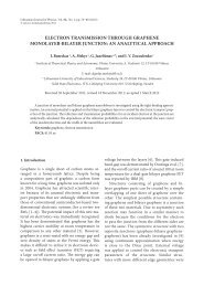
Numerical example<br />
I(t)<br />
60<br />
50<br />
40<br />
30<br />
20<br />
10<br />
0<br />
0 0.2 0.4 0.6 0.8 1 1.2 1.4 1.6<br />
t<br />
Typical signal<br />
P(x)<br />
10 2<br />
10 0<br />
10 -2<br />
10 -4<br />
10 -6<br />
10 -8<br />
10 -10<br />
10 -12<br />
10 -14<br />
10 -16<br />
10 -18<br />
0.1 1 10 100 1000 10000<br />
Distribution of x<br />
x<br />
10 1 0.1 1 10 100 1000 10000<br />
S(f)<br />
10 0<br />
10 -1<br />
10 -2<br />
10 -3<br />
10 -4<br />
10 -5<br />
Power spectral density<br />
f<br />
dx =<br />
(<br />
1 + x min<br />
2x − x<br />
2x max<br />
)x 4 dt + x 5 2 dW t<br />
ν = 3, η = 5 2 , x min = 1, x max = 10 3 .<br />
1/f spectrum.<br />
Julius Ruseckas (Lithuania) <strong>Nonlinear</strong> <strong>stochastic</strong> <strong>differential</strong> <strong>equations</strong> August 28, 2012 20 / 32
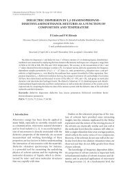
Intermittent behavior of solutions<br />
60<br />
50<br />
40<br />
I(t)<br />
30<br />
20<br />
10<br />
0<br />
0 0.2 0.4 0.6 0.8 1 1.2 1.4 1.6<br />
t<br />
Signals generated by proposed SDE exhibit<br />
intemittent behavior: there are bursts corresponding to large<br />
deviations, separated by laminar phases.<br />
Bursts are characterized by power-law distributions of burst size,<br />
burst duration, <strong>and</strong> interburst time.<br />
Julius Ruseckas (Lithuania) <strong>Nonlinear</strong> <strong>stochastic</strong> <strong>differential</strong> <strong>equations</strong> August 28, 2012 21 / 32
Outline<br />
1 Introduction: 1/f <strong>noise</strong><br />
2 Stochastic <strong>differential</strong> <strong>equations</strong> giving 1/f <strong>noise</strong><br />
3 Some models resulting in proposed SDE<br />
Point processes<br />
Simple model of herding behavior<br />
4 Summary<br />
Julius Ruseckas (Lithuania) <strong>Nonlinear</strong> <strong>stochastic</strong> <strong>differential</strong> <strong>equations</strong> August 28, 2012 22 / 32
Point processes<br />
The signal of the model consists of pulses or events<br />
I(t) = a ∑ k<br />
δ(t − t k )<br />
Point processes arise in different fields such as physics,<br />
economics, ecology, neurology, seismology, traffic flow, financial<br />
systems <strong>and</strong> the Internet.<br />
Julius Ruseckas (Lithuania) <strong>Nonlinear</strong> <strong>stochastic</strong> <strong>differential</strong> <strong>equations</strong> August 28, 2012 23 / 32
Point processes<br />
Let us assume that the signal x is the number of pulses per unit time.<br />
How to obtain equation for inter-event time τ k = t k − t k−1 :<br />
Transform the equation from the variable x to τ = 1/x<br />
Discretize the equation according to Euler-Marujama<br />
approximation<br />
Take time step equal to τ k<br />
Julius Ruseckas (Lithuania) <strong>Nonlinear</strong> <strong>stochastic</strong> <strong>differential</strong> <strong>equations</strong> August 28, 2012 24 / 32
Point processes<br />
Example: equation<br />
dx = σ 2 x 4 dt + σx 5/2 dW<br />
leads to<br />
τ k+1 = τ k + σε k<br />
We obtained a simple r<strong>and</strong>om walk of inter-event time<br />
One of possible origins of 1/f <strong>noise</strong><br />
Brownian motion in time axis leads to 1/f <strong>noise</strong><br />
Julius Ruseckas (Lithuania) <strong>Nonlinear</strong> <strong>stochastic</strong> <strong>differential</strong> <strong>equations</strong> August 28, 2012 25 / 32
Point processes<br />
General case<br />
τ k+1 = τ k + γτ 2µ−1<br />
k<br />
where µ = 5/2 − η, γ = σ 2 (1 − η + ν/2).<br />
+ στ µ k ε k<br />
Used for modeling of the internote interval sequences of the<br />
musical rhythms<br />
D. J. Levitin, P. Chordia, <strong>and</strong> V. Menon, Proc. Natl. Acad. Sci. U.S.A. 109, 3716 (2012).<br />
Julius Ruseckas (Lithuania) <strong>Nonlinear</strong> <strong>stochastic</strong> <strong>differential</strong> <strong>equations</strong> August 28, 2012 26 / 32
Herding model<br />
Simple model describing heterogeneous interacting agens:<br />
fixed number N of agents<br />
each of them can be in state 1 or in state 2<br />
agents do not have memory, dynamics described as a Markov<br />
chain<br />
Julius Ruseckas (Lithuania) <strong>Nonlinear</strong> <strong>stochastic</strong> <strong>differential</strong> <strong>equations</strong> August 28, 2012 27 / 32
Herding model<br />
Transition probabilities per unit time:<br />
p(n → n + 1) = (N − n)(σ 1 + hn)<br />
p(n → n − 1) = n(σ 2 + h(N − n))<br />
n is the number of agents in state 1<br />
N − n is the number of agents in state 2<br />
σ 1 <strong>and</strong> σ 2 are probabilities to change the state spontaneously<br />
h describes herding tendency<br />
non-linear terms represent interaction between agents<br />
connectivity between agents increases with the number of agents<br />
N. The interactions have a global character, the range of the<br />
correlations involves a macroscopic fraction of agents.<br />
Julius Ruseckas (Lithuania) <strong>Nonlinear</strong> <strong>stochastic</strong> <strong>differential</strong> <strong>equations</strong> August 28, 2012 28 / 32
Herding model<br />
Ratio of the number of agents in the state 2 to the number of<br />
agents in the state 1:<br />
y = N − n<br />
n<br />
For large N we can represent the dynamics by SDE<br />
dy = [(2h − σ 1 )y + σ 2 ](1 + y)dt + √ 2hy(1 + y)dW<br />
When y ≫ 1 we get our non-linear SDE with parameters η = 3/2,<br />
ν = 1 + σ 1 /h<br />
If σ 1 = 2h, we obtain 1/f spectrum<br />
J. Ruseckas, B. Kaulakys <strong>and</strong> V. Gontis, EPL 96, 60007 (2011).<br />
Julius Ruseckas (Lithuania) <strong>Nonlinear</strong> <strong>stochastic</strong> <strong>differential</strong> <strong>equations</strong> August 28, 2012 29 / 32
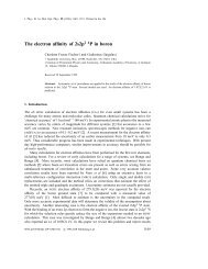
Herding model<br />
10 2 10 -1 10 0 10 1 10 2 10 3 10 4<br />
S(f)<br />
10 1<br />
10 0<br />
10 -1<br />
10 -2<br />
10 -3<br />
10 -4<br />
Power spectral density of the ratio of the numbers of agents.<br />
N = 10 000<br />
Julius Ruseckas (Lithuania) <strong>Nonlinear</strong> <strong>stochastic</strong> <strong>differential</strong> <strong>equations</strong> August 28, 2012 30 / 32<br />
f
Summary<br />
We obtain a class of nonlinear SDEs giving the power-law<br />
behavior of the power spectral density in any desirably wide range<br />
of frequencies<br />
<strong>and</strong> power-law steady state distribution of the signal intensity.<br />
In special cases we obtain other well-known SDEs.<br />
One of the reasons for the appearance of the 1/f spectrum are<br />
scaling properties of the SDE.<br />
Proposed SDEs can be obtained from<br />
point processes with Brownian motion of inter-event time<br />
a simple agent model describing a herding behavior.<br />
Julius Ruseckas (Lithuania) <strong>Nonlinear</strong> <strong>stochastic</strong> <strong>differential</strong> <strong>equations</strong> August 28, 2012 31 / 32
Thank you for your attention!<br />
Julius Ruseckas (Lithuania) <strong>Nonlinear</strong> <strong>stochastic</strong> <strong>differential</strong> <strong>equations</strong> August 28, 2012 32 / 32