integration of cfd and low-order models for combustion ... - IWR

ISABE-2001-1088
INTEGRATION OF CFD AND LOW-ORDER MODELS FOR COMBUSTION
OSCILLATIONS IN AEROENGINES
M. Zhu, A.P. Dowling and K.N.C. Bray
Department of Engineering, University of Cambridge
Cambridge CB2 1PZ, United Kingdom
Tel: +44 1223 332600
Fax: +44 1223 332662
E-mail: mz101@eng.cam.ac.uk
ABSTRACT
The pressure oscillations within combustion chambers of
aeroengines are a major technical challenge to the development
of high performance and low emission propulsion systems. The
oscillations are driven by the resonant interaction between acoustic
waves and unsteady combustion. The acoustic waves vary the
air and fuel supplies and make the combustion unsteady. In return,
unsteady combustion generates yet stronger waves. The
resulting pressure waves can be so intense that they cause unbearable
noise, vibration and even structural damage.
In this paper, an approach integrating a one-dimensional linear
stability analysis and computational fluid dynamics (CFD) is
developed to predict the modes of oscillation in a combustor and
their frequencies and growth rates. Results from the CFD calculation
provide the flame transfer function to describe unsteady
heat release rate. Departure from ideal one dimensional flows are
described by shape factors and we describe a procedure through
which they can be determined. Combined with this information,
low-order models can work out the possible oscillation modes
and their initial growth rates. This work is a further development
of our systematic investigation into the ‘rumble’ phenomenon,
which occurs in aeroengine combustors at idle and sub-idle conditions
and is typically in the range 50-120 Hz. However, the
approach developed here can be used in more general situations
for the analysis of any combustion oscillations.
NOMENCLATURE
a coefficient of IIR filter
b coefficient of IIR filter
c p heat capacity
e total enthalpy
E energy flux
f momentum flux
F non-dimensional shape factor defined in Eq. (8)
H cross-section of combustor
J 1
non-dimensional shape factor defined in Eq. (11)
J 2
non-dimensional shape factor defined in Eq. (12)
m mass flux
p pressure
q rate of heat release
r radial coordinate
R gas constant
S source term
t time
T temperature
u axial velocity
v radial velocity
x axial coordinate
z complex number e iωT
γ ratio of specific heats
ε error
ρ density
ω complex frequency
Superscripts
¯ average over coherent harmonic variation
coherent harmonic perturbation
ˆ complex perturbation

1 INTRODUCTION
The pressure oscillations that can occur within the combustion
chambers of aeroengines are a major technical challenge to
the development of high performance and low emission propulsion
systems. The oscillations are driven by the resonant interaction
between acoustic waves and unsteady combustion. The
acoustic waves vary the air and fuel supplies and make the combustion
unsteady. In return, unsteady combustion generates yet
stronger waves. The pressure waves can become so intense that
they cause unbearable noise, vibration and even structural damage.
It is known that the combustion oscillation is a systemcoupled
phenomenon, which involves the interaction of pressure
waves, unsteady combustion, fuel/air supplies, and geometry of
combustors. In order to fully investigate the phenomenon, a combination
of theoretical analysis, computational fluid dynamics
and experimental work is needed. These techniques combine together
to provide comprehensive information to understand combustion
oscillations and to develop control strategies.
For aeroengines gas turbines, combustors with fuel spray atomizers
are particularly susceptible to a low frequency oscillation
at idle and sub-idle conditions. The frequency of this oscillation
is typically in the range 50-120 Hz and is commonly
called ‘rumble’. In recent years, a systematic program of work
has been undertaken to investigate the ‘rumble’ phenomenon. In
our study, CFD has been employed to calculate unsteady combustion
flows at idle conditions. Through harmonic forcing of
the air or fuel supplies, the main source of the unsteady heat release
has been identified [1]. Excitation by broad-band signals
gives fuller information on the ‘flame transfer function’ between
the rate of unsteady combustion and change in the air mass flow
rate [2]. In the primary zone, an increase in the inlet air mass flow
rate increases the turbulence scalar dissipation rate and hence the
rate of combustion. The increase of air mass flow at the atomizer
leads to a decrease in the inlet fuel droplet size. These smaller
droplets evaporate quickly, increasing the gaseous mixture fraction
in the recirculation zone with a recirculation time delay, and
this also influences the instantaneous rate of combustion and the
location of the burning region. When the boundary conditions
of the combustor are modified to describe the inlet air and fuel
supplies and to include a downstream nozzle, the self-excited oscillations
are established [3]. The causes of the oscillation have
been identified: pressure variations in the combustor chamber alter
the inlet air and fuel spray characteristics, and thereby change
the rate of combustion and generate ‘hot spots’, which convect
downstream. As these ‘hot spots’ accelerate through the downstream
nozzle, an upstream propagating acoustic wave is generated,
which at certain discrete frequencies reinforces the pressure
oscillation.
Although CFD provides a powerful tool to understand combustion
oscillations, there are two drawbacks to relying entirely
on this method. One is that the calculations are very timeconsuming,
and it is not feasible to investigate a wide range of
combustor geometries and flow conditions. The second is that
the calculations are carried out in the time domain. An unstable
operating condition is recognized by tracking the time evolution
until a self-excited oscillation is established. Long simulation
times are necessary to demonstrate stability. These time domain
calculations provide detailed information on the flow motion, but
there is no direct information on the damping factor. The latter
is very useful in determining how close an operating point is to a
instability boundary and in developing control strategies. These
self-excited oscillations involve an almost one-dimensional interaction,
consisting of the convection of ‘hot spots’ downstream
and upstream propagation of a plane acoustic wave. We might
therefore hope to describe it much more quickly through a onedimensional
analysis. Moreover, the stability can be investigate
the linearized equations of motion, where one is interested in
whether disturbances with time dependence e iωt grow or decay
with time.
In this paper, a one-dimensional linear stability analysis and
CFD are integrated to study combustion oscillations. With this
approach, CFD simulation and stability analysis work together to
provide comprehensive information on the mechanism of combustion
oscillation. Results from the CFD calculation provide
the flame transfer function to describe unsteady heat release rate.
Departure from ideal one dimensional flows are described by
shape factors and we describe a procedure through which they
can be determined. Combined with this information, low-order
models can work out the possible oscillation modes and their initial
growth rates. This work is a further development of our systematic
investigation into the ‘rumble’ phenomenon, which occurs
in aeroengine combustors at idle and sub-idle conditions and
is typically in the range 50-120 Hz. However, the approach developed
here can be used in more general situations for the analysis
of any combustion oscillations. In the next section, the areaaveraged
equations for a quasi-one-dimensional stability analysis
are derived through integrating the equations of motion. Three
non-dimensional shape factors are defined to account the effects
of non-uniformity in the radial direction. In section 3, based on
the integrated equations, the equations for mean flow and linear
perturbations are derived from these area-averaged equations.
The determination of the flame transfer function and shape factors
from a single forced CFD calculation are briefly introduced.
In section 4, we integrate the models from this CFD calculation
with the linear perturbation equations. The results are compared
with those from CFD calculation performed with the same inlet
boundary conditions. The sensitivities of the shape factor perturbations
are also investigated. Finally, the conclusions are presented
in section 5.
2 INTEGRATED EQUATIONS
As the ‘rumble’ problem we consider here is a low frequency
oscillation and the wavelengths are long in comparison

©
©
©
©
©
¢
©
¢
©
©
©
©
¢
©
©
¢
¢
©
¡
©
©
©
©
©
©
©
©
©
©
©
©
©
with the combustor diameter, only plane acoustic waves carry
energy. Therefore, it is reasonable to consider one-dimensional
disturbance in stability analysis. The flows we consider are axisymmetric
and the ensemble averaged equations can be written
in two-dimensional form. With the assumption of negligible
molecular transport, and negligible Reynolds stresses and fluxes,
the ensemble averaged conservation equations are
In Eq. (6), the non-uniform influences of momentum transport
in the radial direction are considered through a shape factor
F, which is defined as
F ¢ x¦ t£¥¤
u 2
2
¤
u
ρ H
r
rρu 2 dr
r
r
rρudr 2
§ (8)
r
∂ ¢
ρu£
∂t
∂ρ
∂t
∂ ¡
ρu 2 £
∂x
∂ ¡
∂x
∂ ¢
ρe
∂t t £
∂ ¡ ¢
ρu£
∂x
¡ 1
r
ρue£
∂
∂r
¡ 1
r
∂
∂r
rρv£¥¤ 0 ¦ (1)
¡ rρuv£
¡
rρve£¥¤ §
∂ p
∂x 0 (2)
1 ∂
r ∂r
q (3)
Here and below, we define p, q and ρ as Reynolds ensemble
averages and u, v, T etc as Favre ensemble averages over turbulent
flow fluctuations at x¦ r¦ t£ given . t is the time. x and r
are the spatial coordinates in the axial and radial direction, respectively,
and u and v are the corresponding gas phase ¢ velocity
components; p is the pressure. e t is the internal and mechanical
energy e t ¤
1
c v T
2 u2 α , and e is the total enthalpy given by
¡ ¡
e ¤ e t ¤ ρ p¨
1
c p T
2 u2 α. In this work, the direct effects of
the droplet evaporation and transportation are neglected from the
mass and momentum equations, but they influence q, the ¡ instantaneous
rate of heat release/volume.
The one-dimensional equations can be obtained by the integrating
the Eqs. (1)-(3) over the cross-section. With the assumption
of frictionless slip flows at walls without heat transfer, the
quantities integrated flow equations across the width of a combustor
can be written as
φ ¤
1
H
r
r
rφ dr ¦ and © ψ¤
1
ρ H
r
r
rρψ dr ¦ (4)
where φ represents ρ and q, and ψ represents u, v, u 2 , e t and
e. H © x£¤
r
r rdr, is the cross-sectional area of the combustor,
and is uniform in this study. Integrating Eqs. (1)-(3), onedimensional
conservation equations can be written ¢ as
∂ ¡ 1 ρ ∂
H © © u¤ S ρ
m (5)
¦
∂t H ∂x
¡ ∂ 1 ∂ 2 d p ¡
u ρ
ρ u HF¤ S
∂t H ∂x dx f
(6) ¦
¡ ∂
1 ∂
e ρ
∂t t
e ρ H¤ q S u
e (7) §
H
∂x
where S m , S f
and S e are the sources terms of mass, momentum
and energy due to the primary and secondary air injections, respectively.
For the total energy and total enthalpy, the integrated variable can
be written as
©
e t ¤ c v T
e¥¤ c p
©
1 2 © ¡
F and ¦ (9)
u
2
T J 1
¡ 1
2
u 2 J 2
§ (10)
The dimensionless shape factors J 1
and J 2
are used to describe
the non-uniform influences of the enthalpy and kinetic energy
transports in the radial direction, and are defined as
¢
J 1
t£¥¤ x¦
¢
J 2
t£¥¤ x¦
c p uT
¦ (11)
and¦
c p T u
u 3 ¨
u 3 ¦ (12)
respectively. Although the heat capacity c p and state equation coefficient
R are not uniform within combustion chamber as combustion
alters the components of flow, we find from our later results
that it is accurate enough to treat them as constants.
The shape factors (F, J 1
and J 2
) and the heat release rate
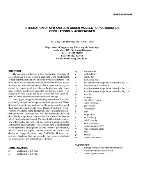
can be obtained from a single CFD forcing q calculation. As
in our previous work, the CFD calculation has been conducted
in the idealized 2D axisymmetric annular combustor shown in
Fig. 1. Fuel and air are injected through inlets 1 and 2 and dilution
air through ports 3-10. The boundary conditions are specified
to be representative of an aero-engine at idle. A contour
plot of a typical mean temperature distribution is shown in Fig. 2
for cross-reference in following discussion. More information
on the CFD algorithm and boundary conditions can be found in
reference [1, 3].
After a steady solution was achieved, the mean ¢
values ¢
of
F , J x£ 1
and x£ J 2
were calculated according to Eqs. (8), x£ (11)
and (12), respectively. The results are shown in Figs. 3, 4 and
5, respectively. These non-dimensional shape factors ¢ would be
unity if the axial velocity and the transported properties were ideally
uniform, i.e. independent of radius r. From Fig. 3, it can be
seen that ¯F is large at the combustor inlet and outlet due to the
high flow velocities that occur near the injectors and open exit,
with virtually stagnant flow outside the main stream. Elsewhere
in the combustor, the flow is relatively uniform, thus ¯F is closer
to unity. The shape factor J 1
is determined not only by flow velocity,
but also by the temperature distribution. Its mean value is

©
©
©
¡
©
©
©
©
©
©
©
©
©
©
©
©
©
©
©
© ¢
©
©
¢
¢
©
©
©
¢
¢
©
©
©
©
©
©
©
©
©
©
©
¢
©
©
©
©
©
©
¢
©
©
©
©
©
©
©
©
©
©
©
(
©
©
©
©
¢
¢
©
©
©
©
¡
©
©
©
©
©
©
©
©
©
©
©
©
¦
shown in Fig. 4. It is interested to see that J¯
1
is less than unity in
the upstream section because here the higher temperature region
is located in the recirculation zone where the velocity is stagnated
or very small. Downstream of the combustion zone the
hot low density gas is differentially accelerated by the pressure
gradient and J¯
1
increases to values greater than unity. As a consequence,
we can see that J¯
1
is continuously increased in Fig. 4.
The small steps in Figs. 3-5 correspond to the effects of the primary
and secondary air injections. The explanation for the shape
factor J 2
, which is shown in Fig. 5, is similar to that for Fig. 3.
The difference is that J¯
2
is much larger at the two boundaries due
to the third power of velocity in Eq. (12) for the kinetic energy
transport.
state, the relationships for flow variables can be written as [4]
u¤ ¯
p¤ ¯
ρ¤ ¯
T ¤ ¯
γJ¯
¯
1
f
2γFJ¯
1
1£ γ J ¯ ¯
2
m
γ 2 ¯
J 2 1
¯ f
2 ¡
2
¢
J¯
2
γ 2
1£ 2 ¯F J¯
1
γ γ
¢
2γ ¯F J¯
1
1£ γ J ¯ ¯
2
m
¯
¯ © m 1£
1
¯ 2 E
(20)
m u ¦ ¯F£¨
£!¦ u m¨
ρ p"¨ £§
¯f ¯ H (21)
¯ H ¯
(22)
¯ R ¯
(23)
3 LINEAR STABILITY ANALYSIS
To consider linear perturbations of one-dimensional flows,
it is convenient to write the governing equations in terms of flux
quantities. Here the mass, momentum, and energy fluxes are defined
as
m ¢ x¦ t£¥¤
f ¢ x¦ t£¤
E ¢ x¦ t£¥¤
r
rρu dr ¤ H © ρ
r
r
r p ρu 2 dr ¤ H ¢© ¡ ©
p ρ
£ ¡ ¢
r
r
rρu c p T u 2¨ 2£ dr ¤
¡ ¢
r
u¦ (13)
ρ
u
u 2 F£¦ (14)
e H ¦ (15)
respectively.
As the linear perturbation theory is considered here, it is sufficient
to investigate perturbation to the mean flow with time dependence
e iωt . The sign of imaginary part of ω determines the
stability, while Re(ω) gives the frequency of the mode. Now time
mean values will be denoted by the overbar and flow quantities
can be expressed as
φ ¢ x¦ t£¤ ¯φ ¢ x£
φ ¢ x¦ t£¦ (16)
where the fluctuating component x¦ t£¤ φ Re ˆφ ¢ x£ e iωt £ Compared
with Eqs. (5)-(7), the conservation equations for steady
flow can be written as
¢ ¢
d
dx ¯ m¥¤
d
dx ¯ ¤ f
d
dx ¯
¯ S m ¦ (17)
p ¯
dH
dx
E¥¤ H ¯ © q ©
¯ ¡
S f
(18)
¦
¯ ¡
S e (19)
§
With the definition of Eqs. (13)-(15) and the equation of
where γ is the ratio of specific heat capacities.
For unsteady parts of the mass flux, momentum flux and energy
flux, we have
¢
¤ f H
ρ ¯
2 ¯ ρ ©
¤ ¢ © ρ m u H ¯
© ©
H E m ¤
1
2 ¯ ¡ 2 ¢
u J2
¯ © ¡
ρ
u u ¯
£¦ u
¡ ©
ρ £ ¡ u
(24)
¯
¯F
u ¯
2 ¡ © F #¦ (25)
p
c p
T ¯ J¯
¡ 1
1
2 ¯ u
ρ ¯
u £ ¯
2 J¯
2
£
©
c p T
J¯
¡
1
c p
T¯
¡
J 1
u ¯
u
¯ J 2
£$§ (26)
With the state equation, the perturbation of flow variables can be
written as
u
ρ ¤
0§ 5 γ 1£ ¯ ¡
J 2 ¢
¤&%
1£ γ
2HR c p
γ 1£ ¯ J 2
m
H ¯ u
¤ p
¤ T ¯
¢
T ©
©
u m u
E u p ρ' u ©
¯F J¯
¯
2
1
J¯
¯
1
f
2HR c p
¯ J 1 H ¯ ¯ ¯
ρ ¯
ρ ¯
ρ ¯
f ¯F ¯ u
¢
p
p ¯
u ¯
u
u ¯
u ¯
m
3 ¯
J 1
¨*% F H ¯ p ¯ ¡
J 1 )(
2
¯F ¯ J 1
ρ ¯
3
J2
¡
u ¯
¦ (27)
¦ (28)
¯ © ¡ ©
u £' m
H
m ¯
u ¯ F
2 ¡
¦ (29)
ρ
£§
¯ ρ
(30)
For linear disturbances whose time dependence is proportional
to e iωt , the equations for the perturbations of mass flux,

©
¢
©
©
©
©
¢
©
©
x¦
¢
©
¢
©
©
©
¡
¡
¡
©
¢
¤
©
momentum flux and energy flux can be written as
d ˆ ©
m
dx
d ˆ f
dx
d
ʤ
dx
iωH ˆ ©
ρ*¦ (31)
¤
iω ˆ ©
m ¤
q+ ˆ
ρ ¯
c v
ˆ
© ¡
p
iωH
© ¢
ρ ˆ
T ˆ
¯ © ¡
dH
dx (32)
¦ ¡
c v T¯
1
2 ¯ 2 u ¯F£
u ˆ ¯F 1 u
2 ¯ 2 ˆF£#§ (33)
¡ u
The unsteady heat release rate is the main driving force of
combustion instability, and when predicting combustion oscillations,
it is important to describe the coupling between this rate of
heat release and the flow. Many models for flame transfer functions
have been described in the literature [4, 5]. In our recent
work, a method for calculating flame transfer functions with CFD
has been developed. Here, CFD was used to calculate the unsteady
flow in the combustor. Through calculations of the forced
unsteady combustion resulting from a specified time-dependent
variation in the air supply, we were able to obtain information
on the transfer function between rate of heat release and the air
flow rate through the atomizer. For one-dimensional analysis, the
heat release rate is obtained by integration across the combustior
section. The ARX model is used in the transfer function calculation
[6]. This means the transfer function at axial position x is
written in the form of an IIR filter, with additional noise, i.e.
q
x¦ nT £¥¤
1
¢ I,
∑ a i x£ m a x¦
0 i-
K
∑
¢
b k
x£
1 k-
q
n i N£ T
n
k£ T
ε ¢ nT £§ (34)
The error ε ¢ t£ is assumed to be uncorrelated to q ¢ x¦ t£ and independent
of frequency. The input signal we used in this work
is the sum of sinusoidal signals, before normalization it can be
written as
¢
m a £¤ nT
K
∑
k- 1
sin ¢ π ¢ n 1£ ω k
t ¡ 2πw ¢ k££¦
and n ¤ 1 . .. N ¦ (35)
where K is the number of sinusoids which are equally spread
over the passband. ω 1
and ω 2
are the lower and upper limits of
¡
the passband, and ω k
¤ ω 1
k ω 2
ω 1
K¦ k ¤ 1 . . . K. w ¢ k£
£¨
describes the phase of the kth sinusoid at ¢ t 0 and is a ¤
random
number chosen from a uniform distribution on the interval
¢ ¢
. After the 0¦ 1 a i
x£ and b k
are obtained, the x£ frequency domain
transfer function of the flame model can be written as
H ¢ ω ¦ x£¤
q ˆ
ω ¦ x£
ˆm a
¢
ω£
1 ¢ I,
∑ a i
x£ z i , i- 0
K ¢
1 ∑ b k
x£ z k , § (36)
1 k-
The integrated mean heat release rate is shown in Fig. 6. The
flame transfer functions at 50 Hz, calculated with I¦ K ¤ 10 and
I¦ K ¤ 30 are shown in Fig. 7. The transfer functions of the shape
factors can be calculated with the same method.
4 RESULTS AND DISCUSSION
The mean values of mass, momentum and energy fluxes can
be calculated through integration of Eqs. (17)-(19) with appropriate
inlet boundary conditions. The results are shown in Figs. 8-
10 are with inlet boundary conditions derived from the CFD results
to aid comparison in this paper. In these figures, three steps
are clearly demonstrated, which correspond to the contributions
from the primary and secondary air injections. In current study,
the source terms S m , S f
and S e are kept as constants in both the
CFD and in the linear analysis. The mean values of flow variables
can be obtained according to Eqs. (20)-(23). The mean values
of temperature and velocity are shown in Figs 11 and 12, respectively.
From Figs. 8-12, we can see that the mean flow results
from one-dimensional analysis are in good agreement with those
from CFD calculations. From Fig. 11, it can be seen that the integrated
temperature is much lower than that within combustion
zone. This is because, at this idle condition, the temperature of
most of the air within combustor is relatively low, although the
local temperature can be as high as 2000 K. For the integrated
velocity, as shown in Fig. 12, three steps due to additional air
injected are clearly demonstrated. The decrease following each
step in mean velocity is the subsequence of the relatively high
density of the cool flow in the recirculation induced by the flow
injection.
The aim of this study is to develop a method whereby a linear
stability analysis can provide a useful tool to predict ‘rumble’.
Our first calculation involved keeping the shape factors
constant (independent of time) and using the flame transfer functions
identified from CFD calculation. In the one-dimensional
analysis, the flame transfer function ˆ describes the relationship
between the unsteady heat release rate with inlet oscilla-
q
tions. We found that this approach led to one-dimensional disturbances
which were significantly different from the area-averaged
CFD results. Therefore, it is necessary to investigate the sensitivities
of the results to the time dependence of the three nondimensional
shape factors. In Eq. (11), the non-dimensional
shape factor J 1 describes the effects of oscillation on the shape

factor describing nonuniformity of the enthalpy transport in the
axial direction. According to the definition, it is determined by
both axial velocity and temperature. That means it also has an
influence on the transport of the entropy wave. It is evident from
Fig. 13 that the position of maximum amplitude of J 1 is in the
recirculation zone. This can be explained by the fact that fluctuation
in the inlet air not only alters the fuel vapor distribution in
this region, it also alters the vorticity, and thus effects the radial
distribution of enthalpy. The results of neglecting J 1 on temperature
and velocity perturbation are shown in Figs. 14 and 15,
respectively. It is seen that there is large difference in the unsteady
temperature and velocity distributions predicted with and
without consideration of J 1 , particularly in combustion region.
From Fig. 15, we can see that there is large difference in the
phase of downstream fluctuation in velocity. This difference can
lead to a large error downstream boundary condition and lead to
significantly different resonant frequencies. Therefore, it is important
to include the fluctuation of J 1
in any stability analysis.
In fact, from our previous work, it is clear that the mechanism
of rumble involves the resonant interaction of the entropy and
acoustic waves. The effects of changes in the radial distribution
of axial transport of enthalpy and hence of entropy are described
by the non-dimensional factor Jˆ
1
. We see that in the prediction
of entropy wave, it is not sufficient to treat the shape function
J 1
as steady. An adjustment is needed to cope with time variations
in radial non-uniformity, particularly due
¢
to the changing
strength of the recirculation vortex. Fortunately, J 1
x¦ t£ ¢ is ¢ influenced
primarily by the inlet air flow rate and Jˆ
1
ω ¦ x£¨ ˆm a ω£ can
be identified from a single forced CFD calculation as described
in section 3.
In Eq. (8), F represents the variation of momentum flux
when the oscillations changes the nonuniformity of the axial velocity.
The magnitude and phase of the relationship between
F and inlet air mass flow rate are shown in Fig. 16. It is seen
x¦ t£
that there are three peaks in the magnitude plot. Comparison with
the flow field contours shows that these ¢ three peaks correspond
to the jets induced by inlets 1 and 2, the combustion recirculation
zone and the downstream contraction, respectively. It means
that the oscillation alters the size or intensity of the jets or vortex,
therefore the axial uniformness of momentum transport. A similar
conclusion can be drawn about the non-dimensional factor
J 2
, which represents the effect of oscillation on the uniformness
of kinetic energy in the radial direction. The comparison of the
results from a one-dimensional analysis with and without considering
F and J 2
are shown in Figs. 17 and 18. It is seen that,
although there are some differences, they are small and the predicted
the magnitude and phase of the flow parameters are quite
comparable. Figures 19 and 20 give time traces of shape factors
J 1
and F at the typical location for forcing at a frequency
50 Hz. It is seen that, in each position, the ratios of magnitude
of oscillation to mean value for J 1
and F are of the same order.
However, as we discussed above, the influence of J 1
on the
one-dimensional flow parameters is much greater than that of F.
This reinforces our argument that the unsteady entropy transport
is more important that those of momentum and kinetic energy.
Hence in a simplified analysis, it is justified to neglect any unsteadiness
in the shape factors F and J 2
, although it should be
retained in J 1
.
5 CONCLUSIONS
In this work, a new approach is developed to give predications
for instability onset and the frequencies of oscillation.
This is based on integrating CFD and low-order models. The
CFD provides the transfer function between the heat release
rate per unit length and air flow rate through the atomizer by
time-dependent calculations of the combustion processes with
specified forced inlet boundary conditions. At the same time
the transfer functions between non-dimensional shape factors
and inlet air flow rate can be calculated. By integrating the
ensemble-averaged conservation equations of motion, quasi-onedimensional
equations for a linear stability analysis are derived.
The effects of any radial non-uniformity on transport of flow parameters
are considered by shape factors, which can be obtained
from the same CFD calculation. Flow quantities can be determined
quickly and straightforwardly by solving the mean flow
and the linear perturbation equations. The amplitude and phase
relationships of temperature and velocity perturbations, which
play an important role in the downstream boundary condition,
have been compared with CFD results for the same inlet boundary
conditions. The results show good agreement. To simplify
the perturbation analysis, the sensitivity to the non-dimensional
shape factors was also investigated. It is shown that the inclusion
of factor J 1
, which represents the effect of radial nonuniformity
on enthalpy transport, is important if the combustion oscillations
are to be predicted correctly. The shape factors F and J 2 , which
represent the momentum and kinetic energy transports, can be
neglected in the linear analysis of combustion oscillation. The
strategy outlined here can be expected to have useful practical
applications if the flame transfer function and the shape factors,
determined from a small number of detailed CFD calculations,
can subsequently be applied to linear stability analyses under a
wider range of conditions. In the future, we will use the method
developed here to predict the instability onset and the frequencies
of oscillation. We anticipate the results will be useful to
understand the combustion oscillation and be helpful in the development
of control strategies.
ACKNOWLEDGMENT
This work was funded by the Engineering and Physical
Sciences Research Council, Rolls-Royce and European
Union GROWTH Program, Research project “ICLEAC: Instability
Control of Low Emission Aero Engine Combustors”

1
2
/
0
Contract(G4RD-CT2000-0215), whose support are gratefully
acknowledged.
3 4 5
REFERENCES
[1] M. Zhu, A.P. Dowling and K.N.C. Bray. Combustion oscillations
in burners with fuel spray atomiser. ASME paper
98–GT–302, Indianapolis, Indiana, June 1999. ASME International
Gas Turbine and Aeroengine Congress and Exhibition.
[2] M. Zhu, A.P. Dowling and K.N.C. Bray. Flame transfer function
calculations for combustion oscillations. ASME paper
2000–GT–374, New Orleans, Louisiana, June 2001. ASME
International Gas Turbine and Aeroengine Congress and Exhibition.
[3] M. Zhu, A.P. Dowling and K.N.C. Bray. Self-excited Oscillations
in Combustors with Spray Atomisers. ASME paper
2000–GT–108, Munich, Germany, May 2000. ASME International
Gas Turbine and Aeroengine Congress and Exhibition.
[4] A. P. Dowling, 1995, “The calculation of thermoacoustic oscillations”,
Journal of Sound and Vibration, 180(4), pp. 557–
581.
[5] A. P. Dowling, 1997, “Nonlinear self-excited oscillations of
a ducted flame”, J. Fluid Mech., 346, pp. 271–290.
[6] L. Ljung. System Identification Toolbox User’s Guide. The
MathWorks Inc., 1991.
r(m)
0.27
0.26
0.25
0.24
0.23
0.22
0.21
0.2
0.19
Figure 1.
Schematic diagram of the geometry.
6 7 /98
0.18
0 0.05 0.1 0.15 0.2
x(m)
/:/
2000
1800
1600
1400
1200
1000
800
600
400
FIGURES
Figure 2. Contour plot of the mean temperature distribution
chamber at idle conditions. The black line indicates the mean
position of the stoichiometric curve and arrows denote the
direction and magnitude of the mean velocity.
4.5
4
3.5
3
mean F
2.5
2
1.5
1
0 0.05 0.1 0.15 0.2 0.25
axial coordinate x(m)
Figure 3.
The mean of dimensionless shape factor ¯F ¢ x£ , which is
defined by Eq. (8).

1.6
mean J 1
1.5
1.4
1.3
1.2
1.1
1
0.9
0.8
0.7
| q |
3.5 x 108
3
2.5
2
1.5
1
0.5
I,K = 10
I,K = 30
0
0 0.02 0.04 0.06 0.08 0.1 0.12 0.14 0.16 0.18 0.2 0.22
Figure 4.
0.6
0 0.05 0.1 0.15 0.2 0.25
axial coordinate x(m)
20
18
16
¢
The mean of dimensionless shape factor J¯
1 , which is x£
defined by Eq. (11).
angle ( q ) deg.
400
300
200
100
0
I,K = 10
I,K = 30
mean J 2
14
12
10
8
6
4
2
Figure 7.
−100
0 0.02 0.04 0.06 0.08 0.1 0.12 0.14 0.16 0.18 0.2 0.22
The transfer function between the heat release rate per
unit length and the air flow rate through the atomizer at a frequency
50 Hz. Identification involves fitting the ARX model of Eq. (34), the
I= >
I= >
solid lines indicate the result from the model K 10 and dash
lines indicate that from the model K 30.
Figure 5.
0
0 0.05 0.1 0.15 0.2 0.25
axial coordinate x(m)
The mean of dimensionless shape factor ¯ J 2 ; x< , which is
defined by Eq. (12).
13
12
11
1D analysis
CFD result
5 x 107 x (m)
q(x) w/m
4.5
4
3.5
3
2.5
2
1.5
mean mass flux
10
9
8
7
6
5
4
1
0.5
0
0 0.025 0.05 0.075 0.1 0.125 0.15 0.175 0.2 0.225
Figure 6.
The mean heat release rate ¯q ; x< per unit length of
combustor.
Figure 8.
3
0 0.05 0.1 0.15 0.2
axial coordinate x(m)
The mean mass flux, where the solid lines indicate the
result from a one-dimensional analysis and dash lines indicate that
from the CFD calculation.

|
2.84 x 104
mean momentum flux
2.835
2.83
2.825
2.82
2.815
2.81
1D analysis
CFD result
mean velocity
65
60
55
50
45
40
1D analysis
CFD result
2.805
35
2.8
0 0.02 0.04 0.06 0.08 0.1 0.12 0.14 0.16 0.18 0.2
axial coordinate x(m)
Figure 9. The mean momentum flux, where the solid lines indicate
the result from a one-dimensional analysis and dash lines indicate
that from the CFD calculation.
8 x 106
30
25
Figure 12.
20
0 0.02 0.04 0.06 0.08 0.1 0.12 0.14 0.16 0.18 0.2 0.22
axial coordinate x(m)
Mean velocity, where the solid lines indicate the result
from a one-dimensional analysis and dash lines indicate that from
the CFD calculation.
7
6
1D analysis
CFD result
mean energy flux
5
4
1.8
1.6
3
1.4
2
1.2
1
Figure 10.
1
0 0.02 0.04 0.06 0.08 0.1 0.12 0.14 0.16 0.18 0.2
axial coordinate x(m)
The mean energy flux, where the solid lines indicate the
result from a one-dimensional analysis and dash lines indicate that
from the CFD calculation.
| J 1
′
0.8
0.6
0.4
0.2
0
0 0.02 0.04 0.06 0.08 0.1 0.12 0.14 0.16 0.18 0.2 0.22
850
800
1D analysis
CFD result
0
−20
750
−40
700
] deg.
−60
mean temperature
650
600
angle [ J 1
′
−80
−100
550
−120
500
−140
0 0.02 0.04 0.06 0.08 0.1 0.12 0.14 0.16 0.18 0.2 0.22
450
Figure 11.
400
0 0.02 0.04 0.06 0.08 0.1 0.12 0.14 0.16 0.18 0.2 0.22
axial coordinate x(m)
Mean temperature, where the solid lines indicate the
result from a one-dimensional analysis and dash lines indicate that
from the CFD calculation.
Figure 13. Magnitude and phase of the transfer function between
shape factor J 1 and air flow rate through the atomizer at a
frequency 50 Hz.

0 0.02 0.04 0.06 0.08 0.1 0.12 0.14 0.16 0.18 0.2 0.22
1800
1600
1400
1200
CFD result
with J1 ′
without J1 ′
2.5
2
1000
| T ′ |
800
600
400
| F ′ |
1.5
1
200
0.5
0
0
0 0.02 0.04 0.06 0.08 0.1 0.12 0.14 0.16 0.18 0.2 0.22
250
200
150
CFD result
with J1 ′
without J1 ′
0
100
−50
angle [ T ′ ] deg.
50
0
−50
−100
angle [ F ′ ] deg.
−100
−150
−150
−200
−200
−250
0 0.02 0.04 0.06 0.08 0.1 0.12 0.14 0.16 0.18 0.2 0.22
Figure 14. Magnitude and phase of the transfer function between
the temperature and air flow rate through the atomizer at a
frequency 50 Hz, where the solid lines indicate the result from the
CFD calculation. The dash lines and dotted-dash lines indicate the
results from one-dimensional analysis with and without J?1 ,
respectively.
Figure 16.
−250
0 0.02 0.04 0.06 0.08 0.1 0.12 0.14 0.16 0.18 0.2 0.22
Magnitude and phase of the transfer function between
shape factor F and air flow rate through the atomizer at a frequency
50 Hz.
450
120
400
CFD result
100
CFD result
with J1 ′
without J1 ′
350
300
with F ′ J2 ′
without F ′ J2 ′
80
250
| T ′ |
200
| u ′ |
60
150
40
100
50
20
0
0 0.02 0.04 0.06 0.08 0.1 0.12 0.14 0.16 0.18 0.2 0.22
0
0 0.02 0.04 0.06 0.08 0.1 0.12 0.14 0.16 0.18 0.2 0.22
200
150
150
CFD result
100
CFD result
with J1 ′
100
with F ′ J2 ′
without F ′ J2 ′
without J1 ′
50
angle [ u ′ ] deg.
50
0
−50
−100
−150
angle [ T ′ ] deg.
0
−50
−100
−150
−200
−250
0 0.02 0.04 0.06 0.08 0.1 0.12 0.14 0.16 0.18 0.2 0.22
Figure 15.
−200
0 0.02 0.04 0.06 0.08 0.1 0.12 0.14 0.16 0.18 0.2 0.22
Magnitude and phase of the transfer function between
the velocity and air flow rate through the atomizer at a frequency
50 Hz, where the solid lines indicate the result from the CFD
calculation. The dash lines and dotted-dash lines indicate the
results from one-dimensional analysis with and without J?1 ,
respectively.
Figure 17. Magnitude and phase of the transfer function between
the temperature and air flow rate through the atomizer at a
frequency 50 Hz, where the solid lines indicate the result from the
CFD calculation. The dash lines and dotted-dash lines indicate the
results from one-dimensional analysis with and F@ without and J@2 ,
respectively.

0 0.02 0.04 0.06 0.08 0.1 0.12 0.14 0.16 0.18 0.2 0.22
35
30
25
CFD result
with F ′ J2 ′
without F ′ J2 ′
20
| u ′ |
15
10
5
0
140
120
100
CFD result
with F ′ J2 ′
without F ′ J2 ′
angle [ u ′ ] deg.
80
60
40
20
2.255 x 105 p 0
( x=0 ) Pa
0
−20
2.25
Figure 18.
−40
0 0.02 0.04 0.06 0.08 0.1 0.12 0.14 0.16 0.18 0.2 0.22
Magnitude and phase of the transfer function between
the velocity and air flow rate through the atomizer at a frequency
50 Hz, where the solid lines indicate the result from the CFD
calculation. The dash lines and dotted-dash lines indicate the
results from one-dimensional analysis with and without F@ and J@2 ,
2.25
respectively.
2.255 x 105 p 0
( x=0 ) Pa
2.245
2.315
2.295
2.275
1.124
1.123
1.122
1.121
1.12
1.69
1.68
F( x 1
, t )
F( x 2
, t )
F( x 3
, t )
2.245
0.78
0.76
0.74
0.72
0.7
1.25
J 1
( x 1
, t )
J 1
( x 2
, t )
1.67
1.66
1.65
0.15 0.16 0.17 0.18 0.19 0.2 0.21
Figure 20.
Sinusoidal changes of the total pressure in the
atomizer air inlet lead to oscillations in the non-dimensional shape
factor F at x 1 A 0B 01m, x 2 A 0B 128m and x 3 A 0B 2m, respectively.
1.24
1.23
1.22
1.25
1.24
1.23
1.22
J 1
( x 3
, t )
1.21
0.15 0.16 0.17 0.18 0.19 0.2 0.21
Figure 19. Sinusoidal changes of the total pressure in the
atomizer air inlet lead to oscillations in the non-dimensional shape
factor J 1 at x 1 A 0B 01m, x 2 A 0B 128m and x 3 A 0B 2m, respectively.