integration of cfd and low-order models for combustion ... - IWR

More documents

Recommendations

Info

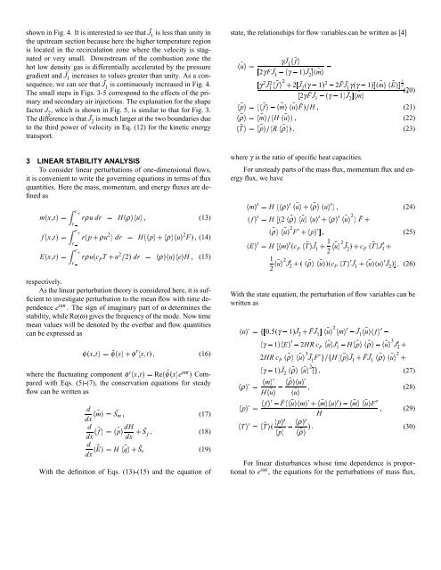
© © © ¡ © © © © © © © © © © © © © © © © ¢ © © ¢ ¢ © © © ¢ ¢ © © © © © © © © © © © ¢ © © © © © © ¢ © © © © © © © © © © © ( © © © © ¢ ¢ © © © © ¡ © © © © © © © © © © © © ¦ shown in Fig. 4. It is interested to see that J¯ 1 is less than unity in the upstream section because here the higher temperature region is located in the recirculation zone where the velocity is stagnated or very small. Downstream of the combustion zone the hot low density gas is differentially accelerated by the pressure gradient and J¯ 1 increases to values greater than unity. As a consequence, we can see that J¯ 1 is continuously increased in Fig. 4. The small steps in Figs. 3-5 correspond to the effects of the primary and secondary air injections. The explanation for the shape factor J 2 , which is shown in Fig. 5, is similar to that for Fig. 3. The difference is that J¯ 2 is much larger at the two boundaries due to the third power of velocity in Eq. (12) for the kinetic energy transport. state, the relationships for flow variables can be written as [4] u¤ ¯ p¤ ¯ ρ¤ ¯ T ¤ ¯ γJ¯ ¯ 1 f 2γFJ¯ 1 1£ γ J ¯ ¯ 2 m γ 2 ¯ J 2 1 ¯ f 2 ¡ 2 ¢ J¯ 2 γ 2 1£ 2 ¯F J¯ 1 γ γ ¢ 2γ ¯F J¯ 1 1£ γ J ¯ ¯ 2 m ¯ ¯ © m 1£ 1 ¯ 2 E (20) m u ¦ ¯F£¨ £!¦ u m¨ ρ p"¨ £§ ¯f ¯ H (21) ¯ H ¯ (22) ¯ R ¯ (23) 3 LINEAR STABILITY ANALYSIS To consider linear perturbations of one-dimensional flows, it is convenient to write the governing equations in terms of flux quantities. Here the mass, momentum, and energy fluxes are defined as m ¢ x¦ t£¥¤ f ¢ x¦ t£¤ E ¢ x¦ t£¥¤ r rρu dr ¤ H © ρ r r r p ρu 2 dr ¤ H ¢© ¡ © p ρ £ ¡ ¢ r r rρu c p T u 2¨ 2£ dr ¤ ¡ ¢ r u¦ (13) ρ u u 2 F£¦ (14) e H ¦ (15) respectively. As the linear perturbation theory is considered here, it is sufficient to investigate perturbation to the mean flow with time dependence e iωt . The sign of imaginary part of ω determines the stability, while Re(ω) gives the frequency of the mode. Now time mean values will be denoted by the overbar and flow quantities can be expressed as φ ¢ x¦ t£¤ ¯φ ¢ x£ φ ¢ x¦ t£¦ (16) where the fluctuating component x¦ t£¤ φ Re ˆφ ¢ x£ e iωt £ Compared with Eqs. (5)-(7), the conservation equations for steady flow can be written as ¢ ¢ d dx ¯ m¥¤ d dx ¯ ¤ f d dx ¯ ¯ S m ¦ (17) p ¯ dH dx E¥¤ H ¯ © q © ¯ ¡ S f (18) ¦ ¯ ¡ S e (19) § With the definition of Eqs. (13)-(15) and the equation of where γ is the ratio of specific heat capacities. For unsteady parts of the mass flux, momentum flux and energy flux, we have ¢ ¤ f H ρ ¯ 2 ¯ ρ © ¤ ¢ © ρ m u H ¯ © © H E m ¤ 1 2 ¯ ¡ 2 ¢ u J2 ¯ © ¡ ρ u u ¯ £¦ u ¡ © ρ £ ¡ u (24) ¯ ¯F u ¯ 2 ¡ © F #¦ (25) p c p T ¯ J¯ ¡ 1 1 2 ¯ u ρ ¯ u £ ¯ 2 J¯ 2 £ © c p T J¯ ¡ 1 c p T¯ ¡ J 1 u ¯ u ¯ J 2 £$§ (26) With the state equation, the perturbation of flow variables can be written as u ρ ¤ 0§ 5 γ 1£ ¯ ¡ J 2 ¢ ¤&% 1£ γ 2HR c p γ 1£ ¯ J 2 m H ¯ u ¤ p ¤ T ¯ ¢ T © © u m u E u p ρ' u © ¯F J¯ ¯ 2 1 J¯ ¯ 1 f 2HR c p ¯ J 1 H ¯ ¯ ¯ ρ ¯ ρ ¯ ρ ¯ f ¯F ¯ u ¢ p p ¯ u ¯ u u ¯ u ¯ m 3 ¯ J 1 ¨*% F H ¯ p ¯ ¡ J 1 )( 2 ¯F ¯ J 1 ρ ¯ 3 J2 ¡ u ¯ ¦ (27) ¦ (28) ¯ © ¡ © u £' m H m ¯ u ¯ F 2 ¡ ¦ (29) ρ £§ ¯ ρ (30) For linear disturbances whose time dependence is proportional to e iωt , the equations for the perturbations of mass flux,
© ¢ © © © © ¢ © © x¦ ¢ © ¢ © © © ¡ ¡ ¡ © ¢ ¤ © momentum flux and energy flux can be written as d ˆ © m dx d ˆ f dx d Ê¤ dx iωH ˆ © ρ*¦ (31) ¤ iω ˆ © m ¤ q+ ˆ ρ ¯ c v ˆ © ¡ p iωH © ¢ ρ ˆ T ˆ ¯ © ¡ dH dx (32) ¦ ¡ c v T¯ 1 2 ¯ 2 u ¯F£ u ˆ ¯F 1 u 2 ¯ 2 ˆF£#§ (33) ¡ u The unsteady heat release rate is the main driving force of combustion instability, and when predicting combustion oscillations, it is important to describe the coupling between this rate of heat release and the flow. Many models for flame transfer functions have been described in the literature [4, 5]. In our recent work, a method for calculating flame transfer functions with CFD has been developed. Here, CFD was used to calculate the unsteady flow in the combustor. Through calculations of the forced unsteady combustion resulting from a specified time-dependent variation in the air supply, we were able to obtain information on the transfer function between rate of heat release and the air flow rate through the atomizer. For one-dimensional analysis, the heat release rate is obtained by integration across the combustior section. The ARX model is used in the transfer function calculation [6]. This means the transfer function at axial position x is written in the form of an IIR filter, with additional noise, i.e. q x¦ nT £¥¤ 1 ¢ I, ∑ a i x£ m a x¦ 0 i- K ∑ ¢ b k x£ 1 k- q n i N£ T n k£ T ε ¢ nT £§ (34) The error ε ¢ t£ is assumed to be uncorrelated to q ¢ x¦ t£ and independent of frequency. The input signal we used in this work is the sum of sinusoidal signals, before normalization it can be written as ¢ m a £¤ nT K ∑ k- 1 sin ¢ π ¢ n 1£ ω k t ¡ 2πw ¢ k££¦ and n ¤ 1 . .. N ¦ (35) where K is the number of sinusoids which are equally spread over the passband. ω 1 and ω 2 are the lower and upper limits of ¡ the passband, and ω k ¤ ω 1 k ω 2 ω 1 K¦ k ¤ 1 . . . K. w ¢ k£ £¨ describes the phase of the kth sinusoid at ¢ t 0 and is a ¤ random number chosen from a uniform distribution on the interval ¢ ¢ . After the 0¦ 1 a i x£ and b k are obtained, the x£ frequency domain transfer function of the flame model can be written as H ¢ ω ¦ x£¤ q ˆ ω ¦ x£ ˆm a ¢ ω£ 1 ¢ I, ∑ a i x£ z i , i- 0 K ¢ 1 ∑ b k x£ z k , § (36) 1 k- The integrated mean heat release rate is shown in Fig. 6. The flame transfer functions at 50 Hz, calculated with I¦ K ¤ 10 and I¦ K ¤ 30 are shown in Fig. 7. The transfer functions of the shape factors can be calculated with the same method. 4 RESULTS AND DISCUSSION The mean values of mass, momentum and energy fluxes can be calculated through integration of Eqs. (17)-(19) with appropriate inlet boundary conditions. The results are shown in Figs. 8- 10 are with inlet boundary conditions derived from the CFD results to aid comparison in this paper. In these figures, three steps are clearly demonstrated, which correspond to the contributions from the primary and secondary air injections. In current study, the source terms S m , S f and S e are kept as constants in both the CFD and in the linear analysis. The mean values of flow variables can be obtained according to Eqs. (20)-(23). The mean values of temperature and velocity are shown in Figs 11 and 12, respectively. From Figs. 8-12, we can see that the mean flow results from one-dimensional analysis are in good agreement with those from CFD calculations. From Fig. 11, it can be seen that the integrated temperature is much lower than that within combustion zone. This is because, at this idle condition, the temperature of most of the air within combustor is relatively low, although the local temperature can be as high as 2000 K. For the integrated velocity, as shown in Fig. 12, three steps due to additional air injected are clearly demonstrated. The decrease following each step in mean velocity is the subsequence of the relatively high density of the cool flow in the recirculation induced by the flow injection. The aim of this study is to develop a method whereby a linear stability analysis can provide a useful tool to predict ‘rumble’. Our first calculation involved keeping the shape factors constant (independent of time) and using the flame transfer functions identified from CFD calculation. In the one-dimensional analysis, the flame transfer function ˆ describes the relationship between the unsteady heat release rate with inlet oscilla- q tions. We found that this approach led to one-dimensional disturbances which were significantly different from the area-averaged CFD results. Therefore, it is necessary to investigate the sensitivities of the results to the time dependence of the three nondimensional shape factors. In Eq. (11), the non-dimensional shape factor J 1 describes the effects of oscillation on the shape
Page 1 and 2: ISABE-2001-1088 INTEGRATION OF CFD
Page 3: © © © © © ¢ © ¢ © © © ©
Page 7 and 8: 1 2 / 0 Contract(G4RD-CT2000-0215),
Page 9 and 10: | 2.84 x 104 mean momentum flux 2.8
Page 11: 0 0.02 0.04 0.06 0.08 0.1 0.12 0.14

integration of cfd and low-order models for combustion ... - IWR

You also want an ePaper? Increase the reach of your titles

Delete template?

Save as template?