Environmental Effects of Increased Atmospheric Carbon Dioxide

Environmental Effects of Increased 

Atmospheric Carbon Dioxide 

Arthur B. Robinson, PhD, Sallie L. Baliunas, PhD, 

Willie Soon, PhD, and Zachary W. Robinson 

ABSTRACT A review of the research literature concerning the 

environmental consequences of increased levels of atmospheric 

carbon dioxide leads to the conclusion that increases during the 

20th Century have produced no deleterious effects upon global 

weather, climate, or temperature. Increased carbon dioxide has, 

however, markedly increased plant growth rates. Predictions of 

harmful climatic effects due to future increases in minor greenhouse 

gases like C% are in error and do not conform to current 

experimental knowledge. 

Summary 

World leaders gathered in Kyoto, Japan, in December 1997 

to consider a world treaty restricting emissions of “greenhouse 

gases,” chiefly carbon dioxide (COz), that are thought to cause 

“global warming” - severe increases in Earth’s atmospheric 

and surface temperatures, with disastrous environmental 

consequences. 

Predictions of global warming are based on computer climate 

modeling, a branch of science still in its infancy. The 

empirical evidence - actual measurements of Earth’s temperature 

- shows no man-made warming trend. Indeed, over the 

past two decades, when CO2 levels have been at their highest, 

global average temperatures have actually cooled slightly. 

To be sure, Cog levels have increased substantially since 

the Industrial Revolution, and are expected to continue doing 

so. It is reasonable to believe that humans have been responsible 

for much of this increase. But the effect on the environment 

is likely to be benign. Greenhouse gases cause plant life, 

and the animal life that depends upon it, to thrive. What 

mankind is doing is liberating carbon from beneath the Earth’s 

surface and putting it into the atmosphere, where it is available 

for conversion into living organisms. 

Rise In Atmospheric Carbon Dioxide 

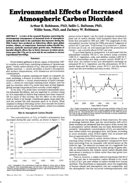
The concentration of C02 in Earth’s atmosphere has 

increased during the past century, as shown in figure 1.’ The 

370 , I 

I 

290 llgOO 

perature increasesP 

280 I I 

I 

1950 1960 1970 1980 1990 2000 

Year 

Fig. 1. Atmospheric C02 concentrations in parts per million by volume ppm, at Mauna 

Loa, Hawaii. These measurements agree well with those at other locations.’ Periodic cycle is 

caused by seasonal variations in C02 absorption by plants. Approximate global level of atmospheric 

CO2 in 1900 and 1940 is also displayed? 

annual cycles in figure 1 are the result of seasonal variations in 

plant use of carbon dioxide. Solid horizontal lines show the 

levels that prevailed in 1900 and 1940.’ The magnitude of this 

atmospheric increase during the 1980s was about 3 gigatons of 

carbon (Gt C) per year.3 Total human CO2 emissions - primarily 

from use of coal, oil, and natural gas and the production of 

cement - are currently about 5.5 Gt C per year. 

To put these figures in perspective, it is estimated that the 

atmosphere contains 750 Gt C; the surface ocean contains 

1,000 Gt C; vegetation, soils, and detritus contain 2,200 Gt C; 

and the intermediate and deep oceans contain 38,000 Gt C.3 

Each year, the surface ocean and atmosphere exchange an 

estimated 90 Gt C; vegetation and the atmosphere, 60 Gt C; 

marine biota and the surface ocean, 50 Gt C; and the surface 

ocean and the intermediate and deep oceans, 100 Gt C3 

0 “k 

26 I I 

Medieml Climate Optimum 

A 

i 

- 

Little Ice Age 

20 ’ I 

3000 2500 2000 1500 1000 500 0 

Years Before Present 

I 

I 

7 1 

Fig. 2. Surface temperatures in the Sargasso Sea (with time resolution of about 50 years) 

ending in 1975 as determined by isotope ratios of marine organism remains in sediment at the 

bottom of the sea? The horizontal line is the average temperature for this 3,000 year period. 

The Little Ice Age and Medieval Climate Optimum were naturally occurring, extended intervals 

of climate departures from the mean. 

So great are the magnitudes of these reservoirs, the rates 

of exchange between them, and the uncertainties with which 

these numbers are estimated that the source of the recent rise 

in atmospheric carbon dioxide has not been determined with 

certaintyP Atmospheric concentrations of Cog are reported to 

have varied widely over geological time, with peaks, according 

to some estimates, some 20-fold higher than at present and 

lows at approximately 18th-Century levels5 

The current increase in carbon dioxide follows a 300-year 

warming trend: Surface and atmospheric temperatures have 

been recovering from an unusually cold period known as the 

Little Ice Age. The observed increases are of a magnitude that 

can, for example, be explained by oceans giving off gases naturally 

as temperatures rise. Indeed, recent carbon dioxide rises 

have shown a tendency to follow rather than lead global tem- 

There is, however, a widely believed hypothesis that the 3 

Gt C per year rise in atmospheric carbon dioxide is the result 

of the 5.5 Gt C per year release of carbon dioxide from human 

activities. This hypothesis is reasonable, since the magnitudes 

of human release and atmospheric rise are comparable, and 

the atmospheric rise has occurred contemporaneously with 

MEDICAL SENTINEL 

VOLUME 3 NUMBER 5 SEPTEMBER~~CTOBER 1998 171 

1 

-_

the increase in production of C02 from human activities since 

the Industrial Revolution. 

, 18 

-1.0 I I 

1750 1800 1850 1900 1950 2000 

Year 

Fig. 3. Moving 11-year average of terrestrial Northern Hemisphere temperatures as 

deviations in “C from the 1951-1970 mean - left axis and darker Solar magnetic cycle 

lengths - right axis and lighter line.” The shorter the magnetic cycle length, the more active, 

and hence brighter, the sun. 

Atmospheric and Surface Temperatures 

In any case, what effect is the rise in C02 having upon the 

global environment? The temperature of the Earth varies naturally 

over a wide range. Figure 2 summarizes, for example, surface 

temperatures in the Sargasso Sea (a region of the Atlantic 

Ocean) during the past 3,000 years.’ Sea surface temperatures 

at this location have varied over a range of about 3.6 degrees 

Celsius (“C) during the past 3,000 years. Trends in these data 

correspond to similar features that are known from the historical 

record. 

13 

1 1 I I I 

1890 1910 1930 1950 1970 1990 

Year 

Fig. 4. Annual mean surface temperatures in the contiguous United States between 1895 

and 1897, as compiled by the National Climate Data Center.” Horizontal line is the 103-year 

mean. The trend line for this 103-year period has a slope of 0.022 “C per decade or 0.22 OC per 

century. The trend line for 1940 to 1997 has a slope of 0.008 “C per decade or 0.08 OC per 

century. 

For example, about 300 years ago, the Earth was experiencing 

the “Little Ice Age.” It had descended into this relatively 

cool period from a warm interval about 1,000 years ago known 

as the “Medieval Climate Optimum.” During the Medieval 

Climate Optimum, temperatures were warm enough to allow 

the colonization of Greenland. These colonies were abandoned 

after the onset of colder temperatures. For the past 300 years, 

global temperatures have been gradually recovering.” As 

shown in figure 2, they are still a little below the average for the 

past 3,000 years. The human historical record does not report 

“global warming” catastrophes, even though temperatures 

have been far higher during much of the last three millennia. 

What causes such variations in Earth’s temperature? The 

answer may be fluctuations in solar activity. Figure 3 shows 

the period of warming from the Little Ice Age in greater detail 

by means of an 11-year moving average of surface temperatures 

in the Northern Hemisphere.’O Also shown are solar 

magnetic cycle lengths for the same period. It is clear that even 

relatively short, half-century-long fluctuations in temperature 

correlate well with variations in solar activity. When the cycles 

are short, the sun is more active, hence brighter; and the Earth 

is warmer. These variations in the activity of the sun are typical 

of stars close in mass and age to the sun.13 

Figure 4 shows the annual average temperatures of the 

United States as compiled by the National Climate Data 

Center.” The most recent upward temperature fluctuation 

from the Little Ice Age (between 1900 and 1940), as shown in 

the Northern Hemisphere record of figure 3, is also evident in 

this record of US. temperatures. These temperatures are now 

near average for the past 103 years, with 1996 and 1997 having 

been the 42nd and 60th coolest years. 

2 0.4 

C 

8 

- 

C 

.- 

9 -0.4 

8 

0.8 

g 0.6 

5 0.4 

E 

0.2 

0) 

0) 

7 0 

h 

6 -0.2 

7 

-0.4 

L t 

c -0.6 

0 

3 

.- -0.8 

s 

o -1 I 

- 

E 0.2 - 

a 

m 

.? 

m 0 - 

rṁ r 

E -0.2 - 

- 

I 

1958 1968 1978 1988 1998 

Year 

Fig. 5. Radiosonde balloon station measurements of global lower tropospheric temperatures 

at 63 stations between latitudes 90 N and 90 S from 1958 to 1996.15 Temperatures are threemonth 

averages and are graphed as deviations from the mean temperature for 1979 to 1996. 

Linear trend line for 1979 to 1996 is shown. The slope is minus 0.060 “C per decade. 

Especially important in considering the effect of changes 

in atmospheric composition upon Earth temperatures are temperatures 

in the lower troposphere - at an altitude of roughly 

4 km. In the troposphere, greenhouse-gas-induced temperature 

changes are expected to be at least as large as at the surfa~e.’~ 

Figure 5 shows global tropospheric temperatures measured by 

weather balloons between 1958 and 1996. They are currently 

near their 40-year mean,15 and have been trending slightly 

downward since 1979. 

0.6 

-0.6 I 

1978 1983 1988 

Year 

1993 1998 

Fig. 6. Satellite Microwave Sounding Unit, MSU, measurements of global lower tropospheric 

temperatures between latitudes 83 N and 83 S from 1979 to 1997.”,’* Temperatures are 

monthly averages and are graphed as deviations from the mean temperature for 1979 to 1996. 

Linear trend line for 1979 to 1997 is shown. The slope of this line is minus 0.047 “C per 

decade. This record of measurements began in 1979. 

I 

172 MEDICAL SENTINEL 

VOLUME 3 NUMBER 5 SEPTEMBER/~CTOBER 1998

.I 

0.4 

0.3 A 

-0.5 ' 

I 

1979 

1984 1989 1994 1999 

Year 

Fig. 7. Global radiosonde balloon temperature (light line)" and global satellite MSU temperature 

(dark line)".'* from figures 5 and 6 plotted with 6-month smoothing. Both sets of data are 

graphed as deviations from their respective means for 1979 to 1996. The 1979 to 1996 slopes of 

the trend lines are minus 0.060 'C per decade for balloon and minus 0.045 for satellite. 

Disregarding uncertainties in surface measurements and 

giving equal weight to reported atmospheric and surface data 

and to 10 and 19 year averages, the mean global trend is minus 

0.07 "C per decade. 

In North America, the atmospheric and surface records 

partly agree (see figure 8)." Even there, however, the atmospheric 

trend is minus 0.01 per decade, while the surface trend 

is plus 0.07 "C per decade. The satellite record, with uniform 

and better sampling, is much more reliable. 

The computer models on which forecasts of global warming 

are based predict that tropospheric temperatures will rise 

at least as much as surface temperatures.14 Because of this, 

and because these temperatures can be accurately measured 

without confusion by complicated effects in the surface 

record, these are the temperatures of greatest interest. The 

global trend shown in figures 5, 6 and 7 provides a definitive 

means of testing the validity of the global warming hypothesis. 

Since 1979, lower-tropospheric temperature measurements 

have also been made by means of microwave sounding 

units (MSUs) on orbiting satellites.16 Figure 6 shows the average 

global tropospheric satellite mea~urements",'~ - the most 

reliable measurements, and the most relevant to the question 

of climate change. 

Figure 7 shows the satellite data from figure 6 superimposed 

upon the weather balloon data from figure 5. The agreement 

of the two sets of data, collected with completely independent 

methods of measurement, verifies their precision. This 

agreement has been shown rigorously by extensive analysi~.'~~~~ 

While tropospheric temperatures have trended downward 

during the past 19 years by about 0.05 "C per decade, it has 

been reported that global surface temperatures trended 

upward by about 0.1 "C per decade.21,22 In contrast to tropospheric 

temperatures, however, surface temperatures are subject 

to large uncertainties for several reasons, including the 

urban heat island effect (illustrated below). 

During the past 10 years, US. surface temperatures have 

trended downward by minus 0.08 "C per decadeI2 while global 

surface temperatures are reported increased by plus 0.03 "C 

per The corresponding weather-balloon and satellite 

tropospheric 10-year trends are minus 0.4 "C and minus 0.3 "C 

per decade, respectively. 

- 

Resent Radiative Hypothesis 1 Hypothesis 2 

GHE Effectof CO, IPCC 

Fig. 9. Qualitative illustration of greenhouse warming. Present: the current greenhouse 

effect from all atmospheric phenomena. Radiative effect of COz: added greenhouse radiative 

effect from doubling CO2 without consideration of other atmospheric components. 

Hypothesis 1 IF'CC hypothetical amplification effect assumed by IF'CC. Hypothesis 2 hypothetical 

moderation effect. 

The Global Warming Hypothesis 

I C 1 

1979 1984 1989 1994 

Years 

Fig. 8. Tropospheric temperature measurements by satellite MSU for North America 

between 30" to 70" N and 75" to 125" W (dark line)""* compared with the surface record for 

this same region (light line)?4 both plotted with 12-month smoothing and graphed as deviations 

from their means for 1979 to 1996. The slope of the satellite MSU trend line is minus 

0.01 "C per decade, while that for the surface trend line is plus 0.07 OC per decade. The correlation 

coefficient for the unsmoothed monthly data in the two sets is 0.92. 

There is such a thing as the greenhouse effect. 

Greenhouse gases such as H20 and C02 in the Earth's atmosphere 

decrease the escape of terrestrial thermal infrared 

radiation. Increasing CO2, therefore, effectively increases 

radiative energy input to the Earth. But what happens to this 

radiative input is complex: It is redistributed, both vertically 

and horizontally, by various physical processes, including 

advection, convection, and diffusion in the atmosphere and 

ocean. 

When an increase in C02 increases the radiative input to 

the atmosphere, how and in which direction does the atmosphere 

respond? Hypotheses about this response differ and 

are schematically shown in figure 9. Without the greenhouse 

effect, the Earth would be about 14 "C The radiative 

contribution of doubling atmospheric C02 is minor, but this 

radiative greenhouse effect is treated quite differently by 

different climate hypotheses. The hypotheses that the IPCC 

has chosen to adopt predict that the effect of C02 is amplified 

by the atmosphere (especially water vapor) to produce a 

large temperature increase.I4 Other hypotheses, shown as 

hypothesis 2, predict the opposite - that the atmospheric 

response will counteract the C02 increase and result in 

insignificant changes in global 

The empirical 

evidence of figures 5-7 favors hypothesis 2. While Cog has 


VOLUME 3 NUMBER 5 SEPTEMBER~~CTOBER 1998 173

120 

100 

i 

j 80 

E 

P 

60 

i% 

5 40 

20 

0 

Ocean Surface North-Swth 

Flux Correction Wnamic 

Humidity MWdS Grenhouse 

(Doubled C02) 

Heat Flux By 

Motlons 

Fig. 10. The radiative greenhouse effect of doubling the concentration of atmospheric CO2 

(right bar) as compared with four of the uncertainties in the computer climate model^.'^^*^ 

increased substantially, the large temperature increase predicted 

by the IPCC models has not occurred (see figure 11). 

The hypothesis of a large atmospheric temperature 

increase from greenhouse gases (GHGs), and further hypotheses 

that temperature increases will lead to flooding, increases 

in storm activity, and catastrophic world-wide climatological 

changes have come to be known as “global warming” - a phe 

nomenon claimed to be so dangerous that it makes necessary 

a dramatic reduction in world energy use and a severe program 

of international rationing of techn01ogy.2~ 

The computer climate models upon which “global warming” 

is based have substantial uncertainties. This is not surprising, 

since the climate is a coupled, non-linear dynamical 

system - in layman’s terms, a very complex one. Figure 10 

summarizes some of the difficulties by comparing the radiative 

CO2 greenhouse effect with correction factors and uncertainties 

in some of the parameters in the computer climate calculations. 

Other factors, too, such as the effects of volcanoes, 

cannot now be reliably computer modeled. 

Figure 11 compares the trend in atmospheric temperatures 

predicted by computer models adopted by the IPCC with 

that actually observed during the past 19 years - those years 

in which the highest atmospheric concentrations of C02 and 

other GHGs have occurred. 

In effect, an experiment has been performed on the Earth 

during the past half-century - an experiment that includes all 

of the complex factors and feedback effects that determine the 

Earth’s temperature and climate. Since 1940, atmospheric 

GHGs have risen substantially. Yet atmospheric temperatures 

have not risen. In fact, during the 19 years with the highest 

atmospheric levels of Cog and other GHGs, temperatures have 

fallen. 

m 

5 04 

E 0.3 

z 0.2 

- 

- 

P m 0.1 - 

r 

O - 

-0.1 

-0.2 

-0.3 

- 

- 

IPCC Projection of 

Global Warming Trend 

u 

-0.4 

1978 1983 1988 1993 1998 

Year 

Fig. 11. Global annual lower tropospheric temperatures as measured by satellite MSU between 

latitudes 83 N and 83 S ”J~ plotted as deviations from the 1979 value. The trend line of these 

experimental measurements is compared with the corresponding trend line predicted by 

International Panel on Climate Change (IPCC) computer climate models.’4 

Not only has the global warming hypothesis failed the 

experimental test; it is theoretically flawed as well. It can 

reasonably be argued that cooling from negative physical and 

biological feedbacks to GHGs will nullify the initial temperature 

The reasons for this failure of the computer climate 

models are subjects of scientific debate. For example, water 

vapor is the largest contributor to the overall greenhouse 

effe~t.~’ It has been suggested that the computer climate 

models treat feedbacks related to water vapor in~orrectly.~~~~~ 

The global warming hypothesis is not based upon the 

radiative properties of the GHGs themselves. It is based entirely 

upon a small initial increase in temperature caused by GHGs 

and a large theoretical amplification of that temperature 

change. Any comparable temperature increase from another 

cause would produce the same outcome from the calculations. 

At present, science does not have comprehensive quantitative 

knowledge about the Earth’s atmosphere. Very few of 

the relevant parameters are known with enough rigor to 

permit reliable theoretical calculations. Each hypothesis must 

be judged by empirical results. The global warming hypothesis 

has been thoroughly evaluated. It does not agree with the data 

and is, therefore. not validated. 

b.’ 

5 

0.8 

0.6 

a, m 

5 0.4 

P 

4- 

g 0.2 

E 

F 

0 

-0.2 

1880 1900 1920 1940 1960 1980 

Years 

f 

370 

340 6 

‘ci 

P 

L 

C 

8 

s 

3108 

0 

’ 

12. Eleven-year moving average of global surface temperature, as estimated by NASA 

G133,33,34 plotted as deviation from 1890 (left axis and light line), as compared with atmospheric 

CO2 (right axis and dark line).” Approximately 82% of the increase in CO2 occurred 

after the temperature maximum in 1940, as is shown in figure 1. 

The new high in temperature estimated by NASA GISS after 1940 is not present in the 

radiosonde balloon measurements or the satellite MSU measurements. It is also not present in 

surface measurements for regions with comprehensive, high-quality temperature record^.'^ 

The United States surface temperature record (see figure 4) gives 1996 and 1997 as the 38th 

and 56th coolest years in the 20th century. Biases and uncertainties, such as that shown in figure 

13. account for this difference. 

Global Warming Evidence 

Aside from computer calculations, two sorts of evidence 

have been advanced in support of the “global warming” 

hypothesis: temperature compilations and statements about 

global flooding and weather disruptions. Figure 12 shows the 

global temperature graph that has been compiled by National 

Aeronautic and Space Administration’s Goddard Institute of 

Space Studies (NASA GISS).23,33,34 This compilation, which is 

shown widely in the press, does not agree with the atmospheric 

record because surface records have substantial uncertainties.36 

Figure 13 illustrates part of the reason. 

The urban heat island effect is only one of several surface 

effects that can confound compiled records of surface temperature. 

Figure 13 shows the size of this effect in, for example, 

the surface stations of California and the problems associated 

with objective sampling. The East Park station, considered the 

best situated rural station in the has a trend since 1940 

of minus 0.055 “C per decade. 

The overall rise of about plus 0.5 “C during the 20th 

280 


VOLGME 3 NUMBER 5 SEPTEMBER/~CTOBER 1998

I 

0.8 

p 0.7 

CD 

0) 

53 0.6 

0 

d 

0.5 

a, 

-0 

3 0.4 

a, 

0 

0.3 

Q 

‘0 

= 0.2 

e! 

4- 

e! 

3 0.1 

P 

a, 

E o 

F 

-0.1 

X 

/ 

K I Y 

10,000 100,000 1,000,000 10,000,000 

Population of County 

Fig. 13. Surface temperature trends for the period of 1940 to 1996 from 107 measuring stations 

in 49 California co~nties.)~.~ After averaging the means of the trends in each county, 

counties of similar population were combined and plotted as closed circles along with the standard 

errors of their means. The six measuring stations in Los Angeles County were used to 

calculate the standard error of that county, which is plotted alone at the county population of 

8.9 million. The “urban heat island effect” on surface measurements is evident. The straight 

line is a least-squares fit to the closed circles. The points marked “X” are the six unadjusted 

station records selected by NASA GISSz3,33,34 for use in their estimate of global temperatures 

as shown in figure 12. 

century is often cited in support of “global warming.”38 Since, 

however, 82% of the C02 rise during the 20th century occurred 

after the rise in temperature (see figures 1 and 12), the C02 

increase cannot have caused the temperature increase. The 

19th century rise was only 13 ppm.’ 

In addition, incomplete regional temperature records have 

been used to support “global warming.” Figure 14 shows an 

example of this, in which a partial record was used in an 

attempt to confirm computer climate model predictions of 

temperature increases from greenhouse gases.4’ A more complete 

record refuted this attern~t.~’ 

Not one of the temperature graphs shown in figures 4 to 7, 

which include the most accurate and reliable surface and 

atmospheric temperature measurements available, both global 

and regional, shows any warming whatever that can be attributed 

to increases in greenhouse gases. Moreover, these data 

show that present day temperatures are not at all unusual 

compared with natural variability, nor are they changing in any 

unusual way. 

\ 

Sea Levels and Storms 

The computer climate models do not make any reliable 

predictions whatever concerning global flooding, storm variability, 

and other catastrophes that have come to be a part of 

the popular definition of “global warming.” (See Chapter 6, 

section 6-5 of reference 14.) Yet several scenarios of impending 

global catastrophe have arisen separately. One of these 

hypothesizes that rising sea levels will flood large areas of 

coastal land. Figure 15 shows satellite measurements of global 

sea level between 1993 and 1997.43 The reported current global 

rate of rise amounts to only about plus 2 mm per year, or plus 

8 inches per century, and even this estimate is probably 

high.43 The trends in rise and fall of sea level in various regions 

cn 

-6 1 

1993 1994 1995 1996 1997 

Year 

Fig. 15. Global sea level measurements from the Topefloseidon satellite altimeter for 1993 

to ~w.4~ The instrument record gives a rate of change of minus 0.2 mm per yea1.4~ However, 

it has been reported that SO-year tide gauge measurements give plus 1.8 mm per year. A 

correction of plus 2.3 mm per year was added to the satellite data based on comparison to 

selected tide gauges to get a value of plus 2.1 mm per year or 8 inches per ce11tury.4~ 

have a wide range of about 100 mm per year with most of the 

globe showing downward t~ends.4~ Historical records show no 

acceleration in sea level rise in the 20th Moreover, 

claims that global warming will cause the Antarctic ice cap to 

melt and sharply increase this rate are not consistent with 

experiment or with theory? 

Similarly, claims that hurricane frequencies and intensities 

have been increasing are also inconsistent with the data. 

Figure 16 shows the number of severe Atlantic hurricanes per 

year and also the maximum wind intensities of those hurricanes. 

Both of these values have been decreasing with time. 

in 

I .V 

p 0.8 

5 0.6 

5 0.4 

% 0.2 

n 

e! 0.0 

3 

5 -0.2 

% -0.4 

E -0.6 

!- 

-0.8 

1955 1960 1965 1970 1975 1980 1985 1990 1995 2000 

Year 

Fig. 14. The solid circles in the oval are tropospheric temperatures for the Southern 

Hemisphere between latitudes 30 S and 60 S, published in 199641 in support of computermodel-projected 

warming. Later in 1996, the study was refuted by a longer set of data, as 

shown by the open circles!z 

1940 1950 1960 1970 1980 1990 2000 

Year 

Fig. 16. Annual numbers of violent hurricanes and maximum attained wind speeds during 

those humcanes in the Atlantic Ocean.46 Slopes of the trend lines are minus 0.25 hurricanes 

per decade and minus 0.33 meters per second maximum attained wind speed per 

decade. 


VOLUME 3 NUMBER 5 SEPTEMBER/~CTOBER 1998 175

As temperatures recover from the Little Ice Age, the more 

extreme weather patterns that characterized that period may 

be trending slowly toward the milder conditions that prevailed 

during the Middle Ages, which enjoyed average temperatures 

about 1°C higher than those of today. Concomitant changes 

are also taking place, such as the receding of glaciers in 

Montana's Glacier National Park. 

Fertilization of Plants 

How high will the carbon dioxide concentration of the 

atmosphere ultimately rise if mankind continues to use coal, 

oil, and natural gas? Since total current estimates of hydrocarbon 

reserves are approximately 2,000 times annual use,47 doubled 

human release could, over a thousand years, ultimately 

be 10,000 Gt C or 25% of the amount now sequestered in the 

oceans. If 90% of this 10,000 Gt C were absorbed by oceans and 

other reservoirs, atmospheric levels would approximately double, 

rising to about 600 parts per million. (This assumes that 

new technologies will not supplant the use of hydrocarbons 

during the next 1,000 years, a pessimistic estimate of technological 

advance.) 

One reservoir that would moderate the increase is especially 

important. Plant life provides a large sink for Cog. Using 

current knowledge about the increased growth rates of plants 

and assuming a doubling of C02 release as compared to current 

emissions, it has been estimated that atmospheric C02 

levels will rise by only about 300 ppm before leveling off.* At 

that level, COP absorption by increased Earth biomass is able 

to absorb about 10 Gt C per year. 

2.0 I I I 

0 500 1000 1500 2000 1000 1500 2000 

Year 

Year 

Fig. 17. Standard normal deviates of tree ring widths for (a) bristlecone pine, limber pine, 

and fox tail pine in the Great Basin of California, Nevada, and Arizona and (b) bristlecone 

pine in Colorado!* The tree ring widths have been normalized so that their means are zero 

and deviations from the mas 

are displayed in units of standard deviation. 

As atmospheric C02 increases, plant growth rates increase. 

Also, leaves lose less water as C02 increases, so that plants are 

able to grow under drier conditions. Animal life, which depends 

upon plant life for food, increases proportionally. 

Figures 17 to 22 show examples of experimentally measured 

increases in the growth of plants. These examples are 

representative of a very large research literature on this subje~t.~%jj 

Since plant response to C02 fertilization is nearly linear 

with respect to C02 concentration over a range of a few hundred 

ppm, as seen for example in figures 18 and 22, it is easy to 

normalize experimental measurements at different levels of 

C02 enrichment. This has been done in figure 23 in order to 

illustrate some C02 growth enhancements calculated for the 

atmospheric increase of about 80 ppm that has already taken 

place, and that expected from a projected total increase of 320 

PPm. 

As figure 17 shows, long-lived (1,000- to 2000-year-old) 

pine trees have shown a sharp increase in growth rate during 

the past half-century. Figure 18 summarizes the increased 

3.2 

2.4 Needles Branches 

Y" 4.8 1 Boles Total ' I 

E 

._ IS) 4.0 - 

a, 

0 

3.2 - 

2.4 - 

1.6 - 

0.8 

0.0 

300 400 500 600 700 800 400 500 600 700 800 900 

Atmospheric CO2 Concentration pprn 

Fig. 18. Young Eldarica pine trees were grown for 23 months under four CO2 concentrations 

and then cut down and weighed. Each point represents an individual tree?' 

Weights of tree parts are as indicated. 

growth rates of young pine seedlings at four C02 levels. Again, 

the response is remarkable, with an increase of 300 ppm more 

than tripling the rate of growth. 

Figure 19 shows the 30% increase in the forests of the 

United States that has taken place since 1950. Much of this 

increase is likely due to the increase in atmospheric C02 that 

has already occurred. In addition, it has been reported that 

Amazonian rain forests are increasing their vegetation by 

about 34,000 moles (900 pounds) of carbon per acre per year,57 

or about two tons of biomass per acre per year. 

Figure 20 shows the effect of C02 fertilization on sour 

orange trees. During the early years of growth, the bark, limbs, 

and fine roots of sour orange trees growing in an atmosphere 

with 700 ppm of COP exhibited rates of growth more than 170% 

greater than those at 400 ppm. As the trees matured, this 

slowed to about 100%. Meanwhile, orange production was 

127% higher for the 700 ppm trees. 

Trees respond to C02 fertilization more strongly than do 

most other plants, but all plants respond to some extent. 

Figure 21 shows the response of wheat grown under wet conditions 

and when the wheat was stressed by lack of water. These 

were open-field experiments. Wheat was grown in the usual 

way, but the atmospheric C02 concentrations of circular sections 

of the fields were increased by means of arrays of computer-controlled 

equipment that released C02 into the air to 

hold the levels as specified. 

While the results illustrated in figures 17-21 are remarkable, 

they are typical of those reported in a very large number 

of studies of the effect of C02 concentration upon the growth 

rates of 

Figure 22 summarizes 279 similar experiments in which 

700 

600 

1950 1960 1970 1980 1990 

Year 

Fig. 19. Inventories of standing hardwood and softwood timber in the United States 

compiled from Forest Statistics of the United States?' 


VOLUME 3 NUMBER 5 SEPTEMBER/~CTOBER 1998

I 

400 

300 - 171% 175% 

127% 

Trunk & Limbs Fine Roots Trunk & Limbs Oranges 

Young Young Mature per Tree 

Orange Trees Orange Trees Orange Trees 

Fig. 20. Relative trunk and limb volumes and iine root biomass of young sour orange trees; 

and trunk and limb volumes and numbers of oranges produced per mature sour orange tree 

per year at 400 ppm CO2 (light bars) and 700 ppm CO (dark The 400 ppm values 

were normalized to 100. The trees were planted in 1887 as one-year-old seedlings. Young 

trunk and limb volumes and fme root biomass were measured in 1990. Mature trunk and limb 

volumes are averages for 1991 to 1996. Orange numbers are averages for 1993 to 1997. 

plants of various types were raised under C02-enhanced conditions. 

Plants under stress from less-than-ideal conditions - a 

common occurrence in nature - respond more to CO2 fertilization. 

The selections of species shown in figure 22 were 

biased toward plants that respond less to CO2 fertilization 

than does the mixture actually covering the Earth, so figure 22 

underestimates the effects of global CO2 enhancement. 

Figure 23 summarizes the wheat, orange tree, and young 

pine tree enhancements shown in figures 21, 20, and 18 with 

two atmospheric CO2 increases - that which has occurred 

since 1800 and is believed to be the result of the Industrial 

Revolution and that which is projected for the next two centuries. 

The relative growth enhancement of trees by CO2 

diminishes with age. Figure 23 shows young trees. 

Clearly, the green revolution in agriculture has already 

benefited from CO2 fertilization; and benefits in the future will 

likely be spectacular. Animal life will increase proportionally as 

shown by studies of 51 terrestrialti3 and 22 aquatic ecosystem~.~~ 

Moreover, as shown by a study of 94 terrestrial ecosystems 

on all continents except Antar~tica,'~ species richness 

(biodiversity) is more positively correlated with productivity 

-the total quantity of plant life per acre - than with anything 

else. 

Discussion 

There are no experimental data to support the hypothesis 

that increases in carbon dioxide and other greenhouse gases 

are causing or can be expected to cause catastrophic changes 

in global temperatures or weather. To the contrary, during the 

20 years with the highest carbon dioxide levels, atmospheric 

temperatures have decreased. 

We also need not worry about environmental calamities, 

even if the current long-term natural warming trend continues. 

The Earth has been much warmer during the past 3,000 years 

without catastrophic effects. Warmer weather extends growing 

seasons and generally improves the habitability of colder 

regions. "Global warming," an invalidated hypothesis, provides 

no reason to limit human production of CO2, CH4, N20, HFCs, 

PFCs, and SFg as has been 

320 

280 

r; 240 

E 

g 200 

J= 

t 

W 

J= 160 

3 

2 

!? 120 

C 

a, 

2 

r? 80 

40 

0 

o Resource Limited And Stressed 

0 Not Resource Limited Or Stressed 

0 300 600 900 1200 1500 

Atmospheric COP Enrichment ppm 

Fig. 22. Summary data from 279 published experiments in which plants of all types were 

grown under paired stressed (open circles) and unstressed (closed circles) conditions.M There 

were 208, 50, and 21 sets at 300, 600, and an average of about 1350 ppm C02, respectively. 

The plant mixture in the 279 studies was slightly biased toward plant types that respond less 

to C02 fertilization than does the actual global mixture and therefore underestimates the 

expected global response. CO enrichment also allows plants to grow in drier regions, further 

increasing the expected globa?response. 

7 

?? 

d 

0 

1 

10000 , "I ~ 

~~ ~ 

I 

0 70 

8000 

s- 6000 

a, 

n 

Is) 

Y 

0 4000 

._ a, 

>- 

._ C 

2000 

0 

370 mm * . C02 

ppm C02 

# 550 

- 

25% 

12% 

Dry Wet Dry Wet 

1992-93 1993-94 

Fig. 21. Grain yields from wheat grown under well watered and poorly watered conditions 

in open field experiments.61'6* Average CO2-induced increases for the two years were 10% for 

wet and 23% for dry conditions. 

Human use of coal, oil, and natural gas has not measurably 

warmed the atmosphere, and the extrapolation of current 

trends shows that it will not significantly do so in the foreseeable 

future. It does, however, release CO2, which accelerates 

the growth rates of plants and also permits plants to grow in 

drier regions. Animal life, which depends upon plants, also 

flour is hes. 

As coal, oil, and natural gas are used to feed and lift from 

poverty vast numbers of people across the globe, more Cog 

will be released into the atmosphere. This will help to maintain 

and improve the health, longevity, prosperity, and productivity 

of all people. 

Human activities are believed to be responsible for the 

rise in Cog level of the atmosphere. Mankind is moving the carbon 

in coal, oil, and natural gas from below ground to the 

atmosphere and surface, where it is available for conversion 

into living things. We are living in an increasingly lush environment 

of plants and animals as a result of the C02 increase. Our 

children will enjoy an Earth with far more plant and animal life 

as that with which we now are blessed. This is a wonderful and 

unexpected gift from the Industrial Revolution. 


VOLUME 3 NUMBER 5 SEPTEMBER/~CTOBER 1998 177

350 

300 

Q 

0 

m 

N, 250 

m 

0 

r 

200 

w 

I 

-0 

% 150 

E 

f 100 

0 

s 

e 

a 

50 

0 

34% 79Q/" 

65% 

DryWheat Wet Wheat Oranges Orange Young 

Trees Pine Trees 

350 1 

280 

W 600 

E 

,a300 - 

41 

N + 

7 

0 c 

250 - 

$ 200 - 

.- N 

E 

8 150 - 

Z 

C 

._ 

4 100 - 

u 

e 

a 50 - 

I 

41 % 

135% 

114% 

L"" ," 

0 L 

Dry Wheat Wet Wheat Oranges Orange Young 

Trees Pine Trees 

Fig. 23. Calculated growth rate enhancement of wheat, young orange and very young 

pine trees already taking place as a result of atmospheric enrichment by C02 during the past 

two centuries (a) and expected to take place as a result of atmospheric enrichment by C02 to 

a level of 600 ppm (b). 

In this case, these values apply to pine trees during their first two years of growth and 

orange trees during their 4th through 10th years of growth. As is shown in figure 20, the effect 

of increased C02 gradually diminishes with tree age, so these values should not be interpreted 

as applicable over the entire tree lifespans. There are no longer-running controlled C02 tree 

experiments. Yet, even 2,000 year old trees still respond significantly as is shown in figure 17. 

References 

1. Keeling, C. D. and Whorf, T. P. (1997) Trends Online: A Compendium of Data 

on Global Change, Carbon Dioxide Information Analysis Center, Oak Ridge 

National Laboratory; [ http://cdiac.esd.ornl.gov/ftp/ndpOOl r7/]. 

2. Idso, S. B. (1989) Carbon Dioxide and Global Change: Earth in Transition, IBR 

Press, 7. 

3. Schimel, D. S. (1995) Global Change Biology 1, 77-91. 

4. Segalstad, T. V. (1998) Global Warming the Continuing Debate, Cambridge 

UK Europ. Sci. and Environ. For., ed. R. Bate, 184-218. 

5. Berner, R. A. (1997) Science 276,544-545. 

6. Kuo, C., Lindberg, C. R., and Thornson, D. J. (1990) Nature 343, 709-714. 

7. Kegwin, L. D. (1996) Science 274, 1504-1508 [Ikeigwin@vhoi.edu]. 

8. Jones, P. D. et. al. (1986) J. Clim. Appl. Meterol. 25, 161-179. 

9. Grovesman, B. S. and Landsberg, H. E. (1979) Geophys. Res. Let. 6,767-769. 

10. Baliunas, S. and Soon, W. (1995) Astrophysical Journal 450, 896-901; 

Christensen, E. and Lassen, K. (1991) Science 254, 698-700; [sbaliunas, 

wsoon@cfa.harvard.edu]. 

11. Lamb, H. H. (1982) Climate, History, and the Modern World, pub New York: 

Methuen. 

12. Brown, W. 0. and Heim, R. R. (1996) National Climate Data Center, Climate 

Variation Bulletin 8, Historical Climatology Series 4-7, Dec.; [http://www. 

ncdcmoaa. gov/ol/documentlibrary/cvb.html/]. 

13. Baliunas, S. L. et. al. (1995) Astrophysical Journal 438, 269-287. 

14. Houghton, J. T. et. al. (1995) Report of the Intergovernmental Panel on 

Climate Change, Cambridge University Press. 

15. Angell, J. K. (1997) Trends Online: A Compendium of Data on Global 

Change, Oak Ridge National Laboratory; [http://cdiac.esd.ornl.gov/ 

ftp/ndp008r4/]. 

16. Spencer, R. W., Christy, J. R., and Grody, N. C. (1990) Journal of Climate 3, 

1111-1128. 

17. Spencer, R. W. and Christy, J. R. (1990) Science 247, 15581562. 

18. Christy, J. R., Spencer, R. W., and Braswell, W. D. (1997) Nature 389, 342; 

Christy, J. R. personal comm; [http://wwwghrc.msfc.nasa.gov/ims-cgi-bin/mkda 

ta?msu2rml90+/pub/data/msu/limb90/chan2r/]. 

19. Spencer, R. W. and Christy, J. R. (1992) Journal of Climate 5,8474366. 

20. Christy, J. R. (1995) Climatic Change 31, 455474. 

21. Jones, P. D. (1994) Geophys. Res. Let. 21, 1149-1152. 

22. Parker, D. E., et. al. (1997) Geophys. Res. Let. 24, 1499-1502. 

23. Hansen, J., Ruedy, R. and Sato, M. (1996) Geophys. Res. Let. 23, 16651668 

[ http://www.giss.nasa.gov/data/gistemp/]. 

24. The Climate Research Unit, East Anglia University, United Kingdom; 

[http://www.cru.uea.ac.uk/advancelOk/climdata.htm/]. 

25. Lindzen, R. S. (1994) Ann. Review Fluid. Mech. 26, 353.379. 

26. Sun, D. Z. and Lindzen, R. S. (1993) Ann. Geophysicae 11,204-215. 

27. Spencer, R. W. and Braswell, W. D. (1997) Bull. Amer. Meteorolog. SOC. 78, 

1097-1106. 

28. Baliunas, S. (1996) Uncertainties in Climate Modeling: Solar Variability and 

Other Factors, Committee on Energy and Natural Resources; United States 

Senate. Lindzen, R. S. (1995), personal communication. 

29. Kyoto Protocol to the United Nations Framework Convention on Climate 

Change (1997). Adoption of this protocol would sharply limit CHG release for 

onefifth of the world's people and nations, including the United States. 

30. Idso, S. B. (1997) in Global Warming: The Science and the Politics, ed. L. 

Jones, The Fraser Institute: Vancouver, 91-112. 

31. Lindzen, R. S. (1996) in Climate Sensitivity of Radiative Perturbations: 

Physical Mechanisms and Their Validation, NATO MI Series 134, ed. H. Le Treut, 

Berlin- Heidelberg: Springer-Verlag, 51-66. 

32. Renno, N. O., Emanuel, K. A,, and Stone, P. H. (1994) J. Geophysical 

Research 99, 14429-14441. 

33. Hansen, J. and Lebedeff, S. (1987) J. Geophysical Research 92,1334513372. 

34. Hansen, J. and Lebedeff, S. (1988) Geophys. Res. Let. 15,323.326. 

35. Christy, J. R. (1997) The Use of Satellites in Global Warming Forecasts, 

George C. Marshall Institute. 

36. Balling, Jr., R. C. The Heated Debate (1992), Pacific Research Institute. 

37. Goodridge, J. D. (1998) private communication. 

38. Schneider, S. H. (1994) Science 263, 341-347. 

39. Goodridge, J. D. (1996) Bulletin of the American Meteorological Society 77, 

3-4; Goodridge, J. D. private communication. 

40. Christy, J. R. and Goodridge, J. D. (1995) Atm. Envir. 29, 1957-1961. 

41. Santer, B. D., et. al. (1996) Nature 382,3945. 

42. Michaels, P. J. and Knappenberger, P. C. (1996) Nature 384, 522-523; 

[pjm8x,pck4s@rootboy.nhes.com]; Weber, G. 0. (1996) Nature 384,523-524; Also, 

Santer, B. D. (1996) Nature 384,524. 

43. Nerem, R. S. et. al. (1997) Geophys. Res. Let. 24, 1331-1334; [nerem@ 

csr.utexas.edu]; Douglas, B. C. (1995) Rev. Ceophys. Supplement 14251432. 

44. Douglas, B. C. (1992) J. Geophysical Research 97, 12699-12706. 

45. Bentley, C. R. (1997) Science 275, 1077-1078; Nicholls, K. W. (1997) Nature 

388,460462. 

46. Landsea, C. W., et. al. (1996) Geophys. Res. Let. 23, 1697-1700; [landsea 

@aoml.noaa.gov]. 

47. Penner, S. S. (1998) Energy - The International Journal, January, in press. 

48. Graybill, D. A. and Idso, S. B. (1993) Global. Biogeochem. Cyc. 7, 81-95. 

49. Kimball, B. A. (1983) Agron. J. 75, 779-788. 

50. Poorter, H. (1993) Vegetatio 104-105, 77-97. 

51. Cure, J. D. and Acock, B. (1986) Agric. For. Meteorol. 8, 127-145. 

52. Gifford, R. M. (1992) Adv. Bioclim. 1,2458. 

53. Mortensen, L. M. (1987) Sci. Hort. 33, 1-25. 

54. Drake, B. G. and Leadley, P. W. (1991) Plant, Cell, and Envir. 14,853-860. 

55. Lawlor, D. W. and Mitchell, R. A. C. (1991) Plant, Cell, and Envir. 14,8074318. 

56. Idso, S. B. and Kimball, B. A. (1994) J. Exper. Botany45, 1669-1692. 

57. Grace, J., et. al. (1995) Science 270, 778780. 

58. Waddell, K. L., Oswald, D. D., and Powell D. S. (1987) Forest Statistics of the 

United States, U. S. Forest Service and Dept. of Agriculture. 

59. Idso, S. B. and Kimball, B. A,, (1997) Global Change Biol. 3,89-96. 

60. Idso, S. B. and Kimball, B. A. (1991) Agr. Forest Meteor. 55,345349. 

61. Kimball, et. al. (1995) Global Change Biology 1,429442. 

62. Pinter, J. P. et. al., (1996) Carbon Dioxide and Terrestrial Ecosystems, ed. G. 

W. Koch and H. A. Mooney, Academic Press. 

63. McNaughton, S. J., Oesterhold, M., Frank. D. A,, and Williams, K. J. (1989) 

Nature 341, 142-144. 

64. Cyr, H. and Pace, M. L. (1993) Nature 361,148150. 

65. Scheiner, S. M. and Rey-Benayas, J. M. (1994) Evol. Ecol. 8, 331-347. 

66. Idso, K. E. and Idso, S. (1974) Agr. and Forest Meteorol. 69, 155203. 

Dr. Arthur B. Robinson and Zachary W. Robinson are 

affiliated with the Oregon Institute of Science and Medicine, 

2251 Dick George Road, Cave Junction OR 97523, 

541-5924142, FAX 541-592-2597, [info@oisrn.org]; Drs. Sallie L. 

Baliunas and Willie Soon are affiliated with the 

George C. Marshall Institute, 1730 K Street, N. W., Suite 905, 

Washington, DC 20006, [info@rnarshall.orgJ. 

178 MEDICAL SENTINEL VOLUME 3 NUMBER 5 SEPTEMBER/~CTOBER 1998

Environmental Effects of Increased Atmospheric Carbon Dioxide

Create successful ePaper yourself

Delete template?

Save as template?