EL2620 Nonlinear Control Lecture notes

EL2620 Nonlinear Control 

Lecture notes 

Karl Henrik Johansson, Bo Wahlberg and Elling W. Jacobsen 

This revision December 2011 

Automatic Control 

KTH, Stockholm, Sweden

Preface 

Many people have contributed to these lecture notes in nonlinear control. 

Originally it was developed by Bo Bernhardsson and Karl Henrik Johansson, 

and later revised by Bo Wahlberg and myself. Contributions and comments 

by Mikael Johansson, Ola Markusson, Ragnar Wallin, Henning Schmidt, 

Krister Jacobsson, Björn Johansson and Torbjörn Nordling are gratefully 

acknowledged. 

Elling W. Jacobsen 

Stockholm, December 2011

EL2620 2011 


Automatic Control Lab, KTH 

• Disposition 

7.5 credits, lp 2 

28h lectures, 28h exercises, 3 home-works 

• Instructors 

Elling W. Jacobsen, lectures and course responsible 

jacobsen@kth.se 

Per Hägg, Farhad Farokhi, teaching assistants 

pehagg@kth.se, farakhi@kth.se 

Hanna Holmqvist, course administration 

hanna.holmqvist@ee.kth.se 

STEX (entrance floor, Osquldasv. 10), course material 

stex@s3.kth.se 

Lecture 1 1 



Lecture 1 

• Practical information 

• Course outline 

• Linear vs Nonlinear Systems 

• Nonlinear differential equations 



Course Goal 

To provide participants with a solid theoretical foundation of nonlinear 

control systems combined with a good engineering understanding 

You should after the course be able to 

• understand common nonlinear control phenomena 

• apply the most powerful nonlinear analysis methods 

• use some practical nonlinear control design methods 



Today’s Goal 

You should be able to 

• Describe distinctive phenomena in nonlinear dynamic systems 

• Mathematically describe common nonlinearities in control 

systems 

• Transform differential equations to first-order form 

• Derive equilibrium points 

Lecture 1 4


Course Information 

• All info and handouts are available at the course homepage at 

KTH Social 

• Compulsory course items 

– 3 homeworks, have to be handed in on time (we are strict on 

this!) 

– 5h written exam on December 11 2012 



Course Outline 

• Introduction: nonlinear models and phenomena, computer 

simulation (L1-L2) 

• Feedback analysis: linearization, stability theory, describing 

functions (L3-L6) 

• Control design: compensation, high-gain design, Lyapunov 

methods (L7-L10) 

• Alternatives: gain scheduling, optimal control, neural networks, 

fuzzy control (L11-L13) 

• Summary (L14) 



Material 

• Textbook: Khalil, Nonlinear Systems, Prentice Hall, 3rd ed., 

2002. Optional but highly recommended. 

• Lecture notes: Copies of transparencies (from previous year) 

• Exercises: Class room and home exercises 

• Homeworks: 3 computer exercises to hand in (and review) 

• Software: Matlab 

Alternative textbooks (decreasing mathematical rigour): 

Sastry, Nonlinear Systems: Analysis, Stability and Control; Vidyasagar, 

Nonlinear Systems Analysis; Slotine & Li, Applied Nonlinear Control; Glad& 

Ljung, Reglerteori, flervariabla och olinjära metoder. 

Only references to Khalil will be given. 

Two course compendia sold by STEX. 



Linear Systems 

Definition: Let M be a signal space. The system S : M → M is 

linear if for all u, v ∈ M and α ∈ R 

S(αu) =αS(u) scaling 

S(u + v) =S(u)+S(v) superposition 

Example: Linear time-invariant systems 

ẋ(t) =Ax(t)+Bu(t), y(t) =Cx(t), x(0) = 0 

y(t) =g(t) ⋆ u(t) = 

Y (s) =G(s)U(s) 

∫ t 

0 

g(τ)u(t − τ)dτ 

Notice the importance to have zero initial conditions 



Linear Systems Have Nice Properties 

Local stability=global stability Stability if all eigenvalues of A (or 

poles of G(s)) are in the left half-plane 

Superposition Enough to know a step (or impulse) response 

Frequency analysis possible Sinusoidal inputs give sinusoidal 

outputs: Y (iω) =G(iω)U(iω) 



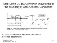
Can the ball move 0.1 meter in 0.1 seconds from steady state? 

Linear model (step response with φ = φ0) gives 

x(t) ≈ 10 t2 2 φ 0 ≈ 0.05φ0 

so that 

φ0 ≈ 0.1 

0.05 

=2rad =114◦ 

Unrealistic answer. Clearly outside linear region! 

Linear model valid only if sin φ ≈ φ 

Must consider nonlinear model. Possibly also include other 

nonlinearities such as centripetal force, saturation, friction etc. 



Linear Models may be too Crude 

Approximations 

Example:Positioning of a ball on a beam 

φ 

x 

Nonlinear model: mẍ(t) =mg sin φ(t), Linear model: ẍ(t) =gφ(t) 



Linear Models are not Rich Enough 

Linear models can not describe many phenomena seen in 

nonlinear systems 


PSfr 


Stability Can Depend on Reference Signal 

Example: Control system with valve characteristic f(u) =u 2 

Motor Valve Process 

r y 

Σ 

1 1 

s (s+1) 2 

−1 

Simulink block diagram: 

1 

s 

1 

u 2 

y 

(s+1)(s+1) 

-1 



STEP RESPONSES 

0.4 

0.2 

Output y 

r =0.2 

0 

4 

0 5 10 15 20 25 30 

Time t 

2 

Output y 

r =1.68 

0 

10 

5 

0 5 10 15 20 25 30 

Time t 

Output y 


Multiple Equilibria 

Example: chemical reactor 

Input 

( 

− 1 

ẋ1 = −x1exp x2 

( 

) 

− 1 ẋ2 = x1exp x2 

f = 0.7, ɛ =0.4 

) 

+ f(1 − x1) 

− ɛf(x2 − xc) 

20 

15 

10 

0 50 100 150 200 

Output 

200 

150 

100 

50 

r =1.72 

0 

0 5 10 15 20 25 30 

Time t 

Stability depends on amplitude of the reference signal! 

(The linearized gain of the valve increases with increasing amplitude) 


Temperature x 2 

Coolant temp x c 

0 

0 50 100 150 200 

time [s] 

Existence of multiple stable equilibria for the same input gives 

hysteresis effect 



Stable Periodic Solutions 

Example: Position control of motor with back-lash 

0 

Constant 

5 

Sum P-controller 

1 

5s 2 +s 

Motor 

y 

Backlash 

-1 

Motor: G(s) = 1 

s(1+5s) 

Controller: K =5 



Back-lash induces an oscillation 

Period and amplitude independent of initial conditions: 

0.5 

0 

Output y 

-0.5 

0.5 

0 10 20 30 40 50 

Time t 

0 

Output y 

-0.5 

0.5 

0 10 20 30 40 50 

Time t 

0 

Output y 

-0.5 

0 10 20 30 40 50 

Time t 

How predict and avoid oscillations? 



Harmonic Distortion 

Example: Sinusoidal response of saturation 

a sin t y(t) = ∑ ∞ 

k=1 A k sin(kt) 

Saturation 

a =1 

10 0 

10 -2 

10 0 

Frequency (Hz) 

a =2 

10 0 

10 -2 

10 0 

Frequency (Hz) 

2 

1 

0 

-1 

-2 

0 1 2 3 4 5 

Time t 

2 

1 

0 

-1 

-2 

0 1 2 3 4 5 

Time t 


Automatic Tuning of PID Controllers 

Relay induces a desired oscillation whose frequency and amplitude 

are used to choose PID parameters 

PID 

Σ A u Process 

y 

T 

Relay 

− 1 

1 

y 

u 

0 

−1 

0 5 10 

Time 


Amplitude y 

Amplitude y 



Example: Electrical power distribution 

Nonlinearities such as rectifiers, switched electronics, and 

transformers give rise to harmonic distortion 

∑ ∞ 

k=2 Energy in tone k 

Total Harmonic Distortion = 

Energy in tone 1 

Example: Electrical amplifiers 

Effective amplifiers work in nonlinear region 

Introduces spectrum leakage, which is a problem in cellular systems 

Trade-off between effectivity and linearity 



Subharmonics 

Example: Duffing’s equation ÿ +ẏ + y − y 3 = a sin(ωt) 

0.5 

0 

-0.5 

1 

0 5 10 15 20 25 30 

Time t 

0.5 

0 

-0.5 

a sin ωt 

y 

-1 

0 5 10 15 20 25 30 

Time t 



Existence Problems 

Example: The differential equation ẋ = x 2 , x(0) = x0 

has solution x(t) = x 0 

1 − x0t , 0 ≤ t< 1 x0 

Solution not defined for tf = 1 x0 

Solution interval depends on initial condition! 

Recall the trick: ẋ = x 2 ⇒ dx 

x = dt 2 

− −1 

Integrate ⇒ −1 

x 0 

x(t) − −1 

x(0) = t ⇒ x(t) = x 1 − x0t 



Nonlinear Differential Equations 

Definition: A solution to 

ẋ(t) =f(x(t)), x(0) = x0 (1) 

over an interval [0,T] is a C 1 function x :[0,T] → R n such that (1) 

is fulfilled. 

• When does there exists a solution? 

• When is the solution unique? 

Example: ẋ = Ax, x(0) = x0, gives x(t) =exp(At)x0 



Finite Escape Time 

Simulation for various initial conditions x0 

Finite escape time of dx/dt = x 2 

5 

4.5 

4 

3.5 

3 

2.5 

x(t) 

2 

1.5 

1 

0.5 

0 

0 1 2 3 4 5 

Time t 



Uniqueness Problems 

Example: ẋ = √ x, x(0) = 0, has many solutions: 

{ (t − C) 

2 /4 t>C 

x(t) = 

0 t ≤ C 

2 

1.5 

1 

0.5 

x(t) 

0 

-0.5 

-1 

0 1 2 3 4 5 

Time t 



Lipschitz Continuity 

Definition: f : R n → R n is Lipschitz continuous if there exists 

L, r > 0 such that for all 

x, y ∈ Br(x0) ={z ∈ R n : ‖z − x0‖ 0 such that 

ẋ(t) =f(x(t)), x(0) = x0 

has a unique solution in Br(x0) over [0, δ]. Proof: See Khalil, 

Appendix C.1. Based on the contraction mapping theorem 

Remarks 

• δ = δ(r, L) 

• f being C 0 is not sufficient (cf., tank example) 

• f being C 1 implies Lipschitz continuity 

(L =maxx∈Br(x0) f ′ (x)) 



State-Space Models 

State x, input u, output y 

General: f(x, u, y, ẋ, ˙u, ẏ, . . .) =0 

Explicit: ẋ = f(x, u), y = h(x) 

Affine in u: ẋ = f(x)+g(x)u, y = h(x) 

Linear: ẋ = Ax + Bu, y = Cx 



Transformation to First-Order System 

Given a differential equation in y with highest derivative dn y 

dt n , 

express the equation in x = 

( 

y 

dy 

... 

dt 

) T 

d n−1 y 

Example: 

dt n−1 

Pendulum 

MR 2¨θ + k ˙θ + MgRsin θ =0 

x = ( θ ˙θ)T gives 

ẋ1 = x2 

ẋ2 = − k 

MR x 2 2 − g R sin x 1 



Transformation to Autonomous System 

A nonautonomous system 

ẋ = f(x, t) 

is always possible to transform to an autonomous system by 

introducing xn+1 = t: 

ẋ = f(x, xn+1) 

ẋn+1 =1 



Equilibria 

Definition: A point (x ∗ ,u ∗ ,y ∗ ) is an equilibrium, if a solution starting 

in (x ∗ ,u ∗ ,y ∗ ) stays there forever. 

Corresponds to putting all derivatives to zero: 

General: f(x ∗ ,u ∗ ,y ∗ , 0, 0,...)=0 

Explicit: 0=f(x ∗ ,u ∗ ), y ∗ = h(x ∗ ) 

Affine in u: 0=f(x ∗ )+g(x ∗ )u ∗ , y ∗ = h(x ∗ ) 

Linear: 0=Ax ∗ + Bu ∗ , y ∗ = Cx ∗ 

Often the equilibrium is defined only through the state x ∗ 



Multiple Equilibria 

Example: Pendulum 

MR 2¨θ + k ˙θ + MgRsin θ =0 

¨θ = ˙θ =0gives sin θ =0and thus θ 

∗ = kπ 

Alternatively in first-order form: 

ẋ1 = x2 

ẋ2 = − k 

MR x 2 2 − g R sin x 1 

ẋ1 =ẋ2 =0gives x ∗ 2 =0and sin(x ∗ 1)=0 



When do we need Nonlinear Analysis & 

Design? 

• When the system is strongly nonlinear 

• When the range of operation is large 

• When distinctive nonlinear phenomena are relevant 

• When we want to push performance to the limit 



Some Common Nonlinearities in Control 

Systems 

|u| 

e u 

Abs 

Math 

Function 

Saturation 

Sign 

Dead Zone 

Look-Up 

Table 

Relay 

Backlash 

Coulomb & 

Viscous Friction 



Next Lecture 

• Simulation in Matlab 

• Linearization 

• Phase plane analysis 





• Wrap-up of Lecture 1: Nonlinear systems and phenomena 

• Modeling and simulation in Simulink 

• Phase-plane analysis 



Analysis Through Simulation 

Simulation tools: 

ODE’s ẋ = f(t, x, u) 

• ACSL, Simnon, Simulink 

DAE’s F (t, ẋ, x, u) =0 

• Omsim, Dymola, Modelica 

http://www.modelica.org 

Special purpose simulation tools 

• Spice, EMTP, ADAMS, gPROMS 





• Model and simulate in Simulink 

• Linearize using Simulink 

• Do phase-plane analysis using pplane (or other tool) 



Simulink 

> matlab 

>> simulink 



An Example in Simulink 

File -> New -> Model 

Double click on Continous 

Transfer Fcn 

Step (in Sources) 

Scope (in Sinks) 

Connect (mouse-left) 

Simulation -> Parameters 

1 

s+1 

Step Transfer Fcn 

Scope 



Save Results to Workspace 

stepmodel.mdl 

Clock 

To Workspace 

1 

s+1 

Step 

Transfer Fcn 

y 

To Workspace1 

u 

To Workspace2 

Check “Save format” of output blocks (“Array” instead of “Structure”) 

>> plot(t,y) 



Choose Simulation Parameters 

Don’t forget “Apply” 



How To Get Better Accuracy 

Modify Refine, Absolute and Relative Tolerances, Integration method 

Refine adds interpolation points: 

Refine = 1 

Refine = 10 

0.8 

0.8 

0.6 

0.6 

0.4 

0.4 

0.2 

0.2 

-0.2 

-0.2 

-0.4 

-0.4 

-0.6 

-0.6 

-0.8 

-0.8 

-1 

-1 

0 1 2 3 4 5 6 7 8 9 10 0 1 2 3 4 5 6 7 8 9 10 


t 

1 

0 

1 

0


Use Scripts to Document Simulations 

If the block-diagram is saved to stepmodel.mdl, 

the following Script-file simstepmodel.m simulates the system: 

open_system(’stepmodel’) 

set_param(’stepmodel’,’RelTol’,’1e-3’) 

set_param(’stepmodel’,’AbsTol’,’1e-6’) 

set_param(’stepmodel’,’Refine’,’1’) 

tic 

sim(’stepmodel’,6) 

toc 

subplot(2,1,1),plot(t,y),title(’y’) 

subplot(2,1,2),plot(t,u),title(’u’) 



Example: Two-Tank System 

The system consists of two identical tank models: 

ḣ =(u − q)/A 

q = a √ 2g √ h 

1 

q 

1 

In 

1/A 

Sum Gain 

1 

s 

Integrator 

f(u) 

Fcn 

2 

h 

1 

In 

q 

In 

h 

Subsystem 

q 

In 

h 

Subsystem2 

1 

Out 


PSfr 


Nonlinear Control System 

Example: Control system with valve characteristic f(u) =u 2 

Motor Valve Process 

r y 

Σ 

1 1 

s (s+1) 2 

−1 

Simulink block diagram: 

1 

s 

1 

u 2 

y 

(s+1)(s+1) 

-1 



Linearization in Simulink 

Linearize about equilibrium (x0,u0,y0): 

>> A=2.7e-3;a=7e-6,g=9.8; 

>> [x0,u0,y0]=trim(’twotank’,[0.1 0.1]’,[],0.1) 

x0 = 

0.1000 

0.1000 

u0 = 

9.7995e-006 

y0 = 

0.1000 

>> [aa,bb,cc,dd]=linmod(’twotank’,x0,u0); 

>> sys=ss(aa,bb,cc,dd); 

>> bode(sys) 



Differential Equation Editor 

dee is a Simulink-based differential equation editor 

>> dee 

Differential Equation 

Editor 

DEE 

deedemo1 deedemo2 deedemo3 deedemo4 

Run the demonstrations 



Homework 1 

• Use your favorite phase-plane analysis tool 

• Follow instructions in Exercise Compendium on how to write the 

report. 

• See the course homepage for a report example 

• The report should be short and include only necessary plots. 

Write in English. 



Phase-Plane Analysis 

• Download ICTools from 

http://www.control.lth.se/˜ictools 

• Down load DFIELD and PPLANE from 

http://math.rice.edu/˜dfield 

This was the preferred tool last year! 





• Stability definitions 

• Linearization 

• Phase-plane analysis 

• Periodic solutions 



Local Stability 

Consider ẋ = f(x) with f(0) = 0 

Definition: The equilibrium x ∗ =0is stable if for all ɛ > 0 there 

exists δ = δ(ɛ) > 0 such that 

‖x(0)‖ < δ ⇒ ‖x(t)‖ < ɛ, ∀t ≥ 0 

x(t) 

δ 

ɛ 

If x ∗ =0is not stable it is called unstable. 





• Explain local and global stability 

• Linearize around equilibria and trajectories 

• Sketch phase portraits for two-dimensional systems 

• Classify equilibria into nodes, focuses, saddle points, and 

center points 

• Analyze stability of periodic solutions through Poincaré maps 



Asymptotic Stability 

Definition: The equilibrium x =0is asymptotically stable if it is 

stable and δ can be chosen such that 

t→∞ 

‖x(0)‖ < δ ⇒ lim 

x(t) =0 

The equilibrium is globally asymptotically stable if it is stable and 

limt→∞ x(t) =0for all x(0). 



Linearization Around a Trajectory 

Let (x0(t),u0(t)) denote a solution to ẋ = f(x, u) and consider 

another solution (x(t),u(t)) = (x0(t)+˜x(t),u0(t)+ũ(t)): 

ẋ(t) =f(x0(t)+˜x(t),u0(t)+ũ(t)) 

= f(x0(t),u0(t)) + ∂f 

∂x (x 0(t),u0(t))˜x(t) 

+ ∂f 

∂u (x 0(t),u0(t))ũ(t)+O(‖˜x, ũ‖ 2 ) 

(x0(t),u0(t)) 

(x0(t)+˜x(t),u0(t)+ũ(t)) 



Example 

h(t) 

m(t) 

ḣ(t) =v(t) 

˙v(t) =−g + veu(t)/m(t) 

ṁ(t) =−u(t) 

Let x0(t) =(h0(t),v0(t),m0(t)) T , u0(t) ≡ u0 > 0, be a solution. 

Then, 

˙˜x(t) = 

⎛ 

0 1 0 

⎜ ⎝ 0 0 − veu 0 

(m0−u0t) 2 

0 0 0 

⎞ 

⎟ ⎠ ˜x(t)+ 

⎛ 

⎝ 

0 

ve 

m0−u0t 

1 

⎞ 

⎠ ũ(t) 



Hence, for small (˜x, ũ), approximately 

˙˜x(t) =A(x0(t),u0(t))˜x(t)+B(x0(t),u0(t))ũ(t) 

where 

A(x0(t),u0(t)) = ∂f 

∂x (x 0(t),u0(t)) 

B(x0(t),u0(t)) = ∂f 

∂u (x 0(t),u0(t)) 

Note that A and B are time dependent. However, if 

(x0(t),u0(t)) ≡ (x0,u0) then A and B are constant. 



Pointwise Left Half-Plane Eigenvalues of 

A(t) Do Not Impose Stability 

A(t) = 

( −1+α cos 

2 t 1 − α sin t cos t 

−1 − α sin t cos t −1+α sin 2 t 

) 

, α > 0 

Pointwise eigenvalues are given by 

λ(t) =λ = α − 2 ± √ α 2 − 4 

2 

which are stable for 0 < α < 2. However, 

( e 

(α−1)t 

cos t e −t sin t 

x(t) = 

−e (α−1)t sin t e −t cos t 

) 

x(0), 

is unbounded solution for α > 1. 



Lyapunov’s Linearization Method 

Theorem: Let x0 be an equilibrium of ẋ = f(x) with f ∈ C 1 . 

Denote A = ∂f (x ∂x 0) and α(A) =maxRe(λ(A)). 

• If α(A) < 0, then x0 is asymptotically stable 

• If α(A) > 0, then x0 is unstable 

The fundamental result for linear systems theory! 

The case α(A) =0needs further investigation. 

The theorem is also called Lyapunov’s Indirect Method. 

A proof is given next lecture. 



Linear Systems Revival 

d 

dt 

[ x 1 

x2 

] 

= A 

[ x 1 

x2 

] 

Analytic solution: x(t) =e At x(0), t ≥ 0. 

If A is diagonalizable, then 

e At = Ve Λt V −1 = [ v1 v2 

] [ e λ 1t 

0 

0 e λ 2t 

] [v 

1 v2 

] −1 

where v1,v2 are the eigenvectors of A (Av1 = λ1v1 etc). 

This implies that 

x(t) =c1e λ 1t v 1 + c2e λ 2t v 2, 

where the constants c1 and c2 are given by the initial conditions 



Example 

The linearization of 

ẋ1 = −x 2 1 + x1 + sin x2 

ẋ2 =cosx2 − x 3 1 − 5x2 

at the equilibrium x0 =(1, 0) T is given by 

( ) −1 1 

A = 

, λ(A) ={−2, −4} 

−3 −5 

x0 is thus an asymptotically stable equilibrium for the nonlinear 

system. 



Example: Two real negative eigenvalues 

Given the eigenvalues λ1 < λ2 < 0, with corresponding 

eigenvectors v1 and v2, respectively. 

Solution: x(t) =c1e λ 1t v 1 + c2e λ 2t v 2 

Slow eigenvalue/vector: x(t) ≈ c2e λ 2t v 2 for large t. 

Moves along the slow eigenvector towards x =0for large t 

Fast eigenvalue/vector: x(t) ≈ c1e λ 1t v 1 + c2v2 for small t. 

Moves along the fast eigenvector for small t 



Phase-Plane Analysis for Linear Systems 

The location of the eigenvalues λ(A) determines the characteristics 

of the trajectories. 

Six cases: 

stable node unstable node saddle point 

Im λi =0: λ1, λ2 < 0 λ1, λ2 > 0 λ1 < 0 < λ2 

Im λi ≠0: Reλi < 0 Reλi > 0 Reλi =0 

stable focus unstable focus center point 



ẋ = 

Example—Unstable Focus 

[ σ −ω 

ω σ 

x(t) =e At x(0) = 

] 

x, σ, ω > 0, λ1,2 = σ ± iω 

[ 1 1 

−i i 

][ ][ e 

σt e 

iωt 

1 1 

0 0 e σt e −iωt −i i 

]−1 

x(0) 

In polar coordinates r = √ x 2 1 + x 2 2 , θ =arctanx 2/x1 

(x1 = r cos θ, x2 = r sin θ): 

ṙ = σr 

˙θ = ω 



Equilibrium Points for Linear Systems 

x2 

x1 

Im λ 

Re λ 



λ1,2 =1± i λ1,2 =0.3 ± i 



Example—Stable Node 

ẋ = 

[ −1 1 

0 −2 

(λ1, λ2) =(−1, −2) and 

] 

x 

[ 

[ 1 −1 

v 1 v2] 

= 

0 1 

] 

v1 is the slow direction and v2 is the fast. 



5 minute exercise: What is the phase portrait if λ1 = λ2? 

Hint: Two cases; only one linear independent eigenvector or all 

vectors are eigenvectors 



Fast: x2 = −x1 + c3 

Slow: x2 =0 



Phase-Plane Analysis for Nonlinear Systems 

Close to equilibrium points “nonlinear system” ≈ “linear system” 

Theorem: Assume 

ẋ = f(x) =Ax + g(x), 

with lim‖x‖→0 ‖g(x)‖/‖x‖ =0. If ż = Az has a focus, node, or 

saddle point, then ẋ = f(x) has the same type of equilibrium at the 

origin. 

Remark: If the linearized system has a center, then the nonlinear 

system has either a center or a focus. 



How to Draw Phase Portraits 

By hand: 

1. Find equilibria 

2. Sketch local behavior around equilibria 

3. Sketch (ẋ1, ẋ2) for some other points. Notice that 

dx2 

dx1 

= ẋ1 

ẋ2 

4. Try to find possible periodic orbits 

5. Guess solutions 

By computer: 

1. Matlab: dee or pplane 



Phase-Plane Analysis of PLL 

Let (x1,x2) =(θ out , ˙θ out ), K, T > 0, and θ in (t) ≡ θ in . 

ẋ1(t) =x2(t) 

ẋ2(t) =−T −1 x2(t)+KT −1 sin(θ in − x1(t)) 

Equilibria are (θ in + nπ, 0) since 

ẋ1 =0⇒ x2 =0 

ẋ2 =0⇒ sin(θin − x1) =0⇒ x1 = θ in + nπ 



Phase-Locked Loop 

A PLL tracks phase θ in (t) of a signal s in (t) =A sin[ωt + θ in (t)]. 

s in 

Phase 

“θout ” 

Detector Filter VCO 

− 

e K 

sin(·) 

1+sT 

θ in θout 

˙θout 

1 

s 



Classification of Equilibria 

Linearization gives the following characteristic equations: 

n even: 

λ 2 + T −1 λ + KT −1 =0 

K>(4T ) −1 gives stable focus 

0


Phase-Plane for PLL 

(K, T) =(1/2, 1): focuses ( 2kπ, 0 ) , saddle points ( (2k + 1)π, 0 ) 



Periodic solution: Polar coordinates. 

x1 = r cos θ ⇒ ẋ1 =cosθṙ − r sin θ ˙θ 

implies 

( ṙ 

Now, from (1) 

x2 = r sin θ ⇒ ẋ2 =sinθṙ + r cos θ ˙θ 

˙θ 

) 

= 1 r 

( r cos θ r sin θ 

− sin θ cos θ 

)( 

ẋ1 

ẋ1 = r(1 − r 2 )cosθ − r sin θ 

ẋ2 

) 

gives 

Only r =1is a stable equilibrium! 

ẋ2 = r(1 − r 2 )sinθ + r cos θ 

ṙ = r(1 − r 2 ) 

˙θ =1 



Periodic Solutions 

Example of an asymptotically stable periodic solution: 

ẋ1 = x1 − x2 − x1(x 2 1 + x 2 2) 

ẋ2 = x1 + x2 − x2(x 2 1 + x 2 2) 

(1) 



A system has a periodic solution if for some T>0 

x(t + T )=x(t), ∀t ≥ 0 

A periodic orbit is the image of x in the phase portrait. 

• When does there exist a periodic solution? 

• When is it stable? 

Note that x(t) ≡ const is by convention not regarded periodic 



Flow 

The solution of ẋ = f(x) is sometimes denoted 

φt(x0) 

to emphasize the dependence on the initial point x0 ∈ R n 

φt(·) is called the flow. 



Existence of Periodic Orbits 

A point x ∗ such that P (x ∗ )=x ∗ corresponds to a periodic orbit. 

P (x ∗ )=x ∗ 

x ∗ is called a fixed point of P . 



Poincaré Map 

Assume φt(x0) is a periodic solution with period T . 

Let Σ ⊂ R n be an n − 1-dim hyperplane transverse to f at x0. 

Definition: The Poincaré map P : Σ → Σ is 

P (x) =φτ(x)(x) 

where τ(x) is the time of first return. 

Σ 

P (x) 

x φt(x) 



1 minute exercise: What does a fixed point of P k corresponds to? 



Stable Periodic Orbit 

The linearization of P around x ∗ gives a matrix W such that 

P (x) ≈ Wx 

if x is close to x ∗ . 

• λj(W )=1for some j 

• If |λi(W )| < 1 for all i ≠ j, then the corresponding periodic 

orbit is asymptotically stable 

• If |λi(W )| > 1 for some i, then the periodic orbit is unstable. 



The Poincaré map is 

P (r0, θ0) = 

( [1 + (r 

−2 

0 − 1)e −2·2π ] −1/2 

θ0 +2π 

) 

(r0, θ0) =(1, 2πk) is a fixed point. 

The periodic solution that corresponds to (r(t), θ(t)) = (1,t) is 

asymptotically stable because 

W = dP 

( e 

−4π 

d(r0, θ0) (1, 2πk) = 0 

0 1 

) 

⇒ Stable periodic orbit (as we already knew for this example) ! 



Example—Stable Unit Circle 

Rewrite (1) in polar coordinates: 

ṙ = r(1 − r 2 ) 

˙θ =1 

Choose Σ = {(r, θ) : r>0, θ =2πk}. 

The solution is 

φt(r0, θ0) = 

( 

[1 + (r 0 −2 − 1)e −2t ] −1/2 ,t+ θ0 

) 

First return time from any point (r0, θ0) ∈ Σ is 

τ(r0, θ0) =2π. 





• Input–output stability 

u y 

S 



r y 

G(s) 

− 

History 

f(y) 

y 

f(·) 

For what G(s) and f(·) is the closed-loop system stable? 

• Luré and Postnikov’s problem (1944) 

• Aizerman’s conjecture (1949) (False!) 

• Kalman’s conjecture (1957) (False!) 

• Solution by Popov (1960) (Led to the Circle Criterion) 





• derive the gain of a system 

• analyze stability using 

– Small Gain Theorem 

– Circle Criterion 

– Passivity 



Gain 

Idea: Generalize the concept of gain to nonlinear dynamical systems 

u y 

S 

The gain γ of S is the largest amplification from u to y 

Here S can be a constant, a matrix, a linear time-invariant system, etc 

Question: How should we measure the size of u and y? 



Norms 

A norm ‖ · ‖ measures size 

Definition: 

A norm is a function ‖ · ‖ : Ω → R + , such that for all x, y ∈ Ω 

• ‖x‖ ≥0 and ‖x‖ =0 ⇔ x =0 

• ‖x + y‖ ≤‖x‖ + ‖y‖ 

• ‖αx‖ = |α|·‖x‖, for all α ∈ R 

Examples: 

Euclidean norm: ‖x‖ = √ x 2 1 + ···+ x 2 n 

Max norm: ‖x‖ =max{|x1|,...,|xn|} 



Eigenvalues are not gains 

The spectral radius of a matrix M 

ρ(M) =max 

i 

|λi(M)| 

is not a gain (nor a norm). 

Why? What amplification is described by the eigenvalues? 



Gain of a Matrix 

Every matrix M ∈ C n×n has a singular value decomposition 

M = UΣV ∗ 

where 

Σ = diag {σ1,...,σn} ; U ∗ U = I ; V ∗ V = I 

σi - the singular values 

The “gain” of M is the largest singular value of M : 

‖Mx‖ 

σmax(M) =σ1 =sup 

x∈R n ‖x‖ 

where ‖ · ‖ is the Euclidean norm. 



Signal Norms 

A signal x is a function x : R + → R. 

A signal norm ‖ · ‖k is a norm on the space of signals x. 

Examples: 

2-norm (energy norm): ‖x‖2 = 

√ ∫ ∞ 

|x(t)| 

0 2 dt 

sup-norm: ‖x‖∞ =sup t∈R + |x(t)| 



Parseval’s Theorem 

L2 denotes the space of signals with bounded energy: ‖x‖2 < ∞ 

Theorem: If x, y ∈ L2 have the Fourier transforms 

X(iω) = 

then ∫ ∞ 

In particular, 

0 

∫ ∞ 

0 

‖x‖ 2 2 = 

e −iωt x(t)dt, Y (iω) = 

y(t)x(t)dt = 1 

2π 

∫ ∞ 

0 

∫ ∞ 

−∞ 

|x(t)| 2 dt = 1 

2π 

∫ ∞ 

0 

Y ∗ (iω)X(iω)dω. 

∫ ∞ 

−∞ 

e −iωt y(t)dt, 

|X(iω)| 2 dω. 

The power calculated in the time domain equals the power calculated 

in the frequency domain 



2 minute exercise: Show that γ(S1S2) ≤ γ(S1)γ(S2). 

u y 

S2 S1 



System Gain 

A system S is a map from L2 to L2: y = S(u). 

u y 

S 

The gain of S is defined as γ(S) =sup 

u∈L2 

‖y‖2 

‖u‖2 

=sup 

u∈L2 

‖S(u)‖2 

‖u‖2 

Example: The gain of a scalar static system y(t) =αu(t) is 

γ(α) =sup 

u∈L2 

‖αu‖2 

‖u‖2 

=sup 

u∈L2 

|α|‖u‖2 

‖u‖2 

= |α| 



Gain of a Static Nonlinearity 

Lemma: A static nonlinearity f such that |f(x)| ≤ K|x| and 

f(x ∗ )=Kx ∗ has gain γ(f) =K. 

Kx 

x ∗ 

f(x) 

u(t) f(·) y(t) 

x 

Proof: ‖y‖ 2 2 = ∫ ∞ 

f 2( u(t) ) dt ≤ ∫ ∞ 

K 2 u 2 (t)dt = K 2 ‖u‖ 2 0 0 2 , 

where u(t) =x ∗ , t ∈ (0, 1), gives equality, so 

γ(f) =sup 

u∈L2 

‖y‖2/ 

‖u‖ 2 = K 



Gain of a Stable Linear System 

Lemma: 

10 

γ(G) 1 

|G(iω)| 

10 0 

γ ( G ) =sup 

u∈L2 

‖Gu‖2 

‖u‖2 

= sup 

ω∈(0,∞) 

|G(iω)| 

10 -1 

10 -2 

10 -1 10 0 10 1 

Proof: Assume |G(iω)| ≤ K for ω ∈ (0, ∞) and |G(iω ∗ )| = K 

for some ω ∗ . Parseval’s theorem gives 

‖y‖ 2 2 = 1 

2π 

= 1 

2π 

∫ ∞ 

−∞ 

∫ ∞ 

−∞ 

|Y (iω)| 2 dω 

|G(iω)| 2 |U(iω)| 2 dω ≤ K 2 ‖u‖ 2 2 

Arbitrary close to equality by choosing u(t) close to sin ω ∗ t. 



The Small Gain Theorem 

r1 

e1 

S1 

S2 

e2 

r2 

Theorem: Assume S1 and S2 are BIBO stable. If γ(S1)γ(S2) < 1, 

then the closed-loop system is BIBO stable from (r1,r2) to (e1,e2) 



BIBO Stability 

Definition: 

S is bounded-input bounded-output (BIBO) stable if γ(S) < ∞. 

u y 

S γ ( S ) =sup 

u∈L2 

‖S(u)‖2 

‖u‖2 

Example: If ẋ = Ax is asymptotically stable then 

G(s) =C(sI − A) −1 B + D is BIBO stable. 



Example—Static Nonlinear Feedback 

r y 

G(s) 

− 

Ky 

f(y) 

y 

f(·) 

G(s) = 

2 

(s +1) , 0 ≤ f(y) 

2 y 

≤ K, ∀y ≠0, f(0) = 0 

γ(G) =2and γ(f) ≤ K. 

Small Gain Theorem gives BIBO stability for K ∈ (0, 1/2). 



“Proof” of the Small Gain Theorem 

‖e1‖2 ≤‖r1‖2 + γ(S2)[‖r2‖2 + γ(S1)‖e1‖2] 

gives 

‖e1‖2 ≤ ‖r 1‖2 + γ(S2)‖r2‖2 

1 − γ(S2)γ(S1) 

γ(S2)γ(S1) < 1, ‖r1‖2 < ∞, ‖r2‖2 < ∞ give ‖e1‖2 < ∞. 

Similarly we get 

‖e2‖2 ≤ ‖r 2‖2 + γ(S1)‖r1‖2 

1 − γ(S1)γ(S2) 

so also e2 is bounded. 

Note: Formal proof requires ‖ · ‖2e, see Khalil 



The Nyquist Theorem 

1 

From: U(1) 

G(s) 0 

-0.5 

-1 

− G(s) -1 -0.5 0 0.5 1 

0.5 

To: Y(1) 


Small Gain Theorem can be Conservative 

Let f(y) =Ky in the previous example. Then the Nyquist Theorem 

proves stability for all K ∈ [0, ∞), while the Small Gain Theorem 

only proves stability for K ∈ (0, 1/2). 

r y 

G(s) 

− 

1 

0.5 

0 

f(·) 

-0.5 

-1 

G(iω) 

-1 -0.5 0 0.5 1 1.5 2 


Theorem: If G has no poles in the right half plane and the Nyquist 

curve G(iω), ω ∈ [0, ∞), does not encircle −1, then the 

closed-loop system is stable. 



r y 

G(s) 

− 

The Circle Criterion 

k2y f(y) 

k1y 

y 

− 1 k1 

− 1 k2 

f(·) 

G(iω) 

Theorem: Assume that G(s) has no poles in the right half plane, and 

0 ≤ k1 ≤ f(y) 

y 

≤ k2, ∀y ≠0, f(0) = 0 

If the Nyquist curve of G(s) does not encircle or intersect the circle 

defined by the points −1/k1 and −1/k2, then the closed-loop 

system is BIBO stable. 



Example—Static Nonlinear Feedback (cont’d) 

Ky 

f(y) 

1 

y 

0.5 

0 

-0.5 

− 1 K 

G(iω) 

-1 

-1 -0.5 0 0.5 1 1.5 2 

The “circle” is defined by −1/k1 = −∞ and −1/k2 = −1/K. 

Since 

min Re G(iω) =−1/4 

the Circle Criterion gives that the system is BIBO stable if K ∈ (0, 4). 



˜r1 

˜G(s) 

−k 

− ˜f(·) 

r2 

R 

1 

G(iω) 

Small Gain Theorem gives stability if | ˜G(iω)|R R 



Proof of the Circle Criterion 

Let k =(k1 + k2)/2, ˜f(y) =f(y) − ky, and ˜r1 = r1 − kr2: 

∣ ∣ ∣∣∣ ˜f(y) ∣∣∣ 

≤ k 2 − k1 

=: R, ∀y ≠0, ˜f(0) = 0 

y 2 

r1 e1 

y2 

G(s) 

−f(·) 

y1 

e2 r2 

˜G −k 

˜r1 

G 

− ˜f(·) 

y1 

r2 



The curve G −1 (iω) and the circle {z ∈ C : |z + k| >R} mapped 

through z ↦→ 1/z gives the result: 

−k2 − k1 

− 1 k1 

− 1 k2 

Note that 

R 

G 

1+kG 

1 

G(iω) 

is stable since −1/k is inside the circle. 

G(iω) 

Note that G(s) may have poles on the imaginary axis, e.g., 

integrators are allowed 



Passivity and BIBO Stability 

The main result: Feedback interconnections of passive systems are 

passive, and BIBO stable (under some additional mild criteria) 



Passive System 

u y 

S 

Definition: Consider signals u, y :[0,T] → R m . The system S is 

passive if 

〈y, u〉T ≥ 0, for all T>0 and all u 

and strictly passive if there exists ɛ > 0 such that 

〈y, u〉T ≥ ɛ(|y| 2 T + |u| 2 T ), for all T>0 and all u 

Warning: There exist many other definitions for strictly passive 



Scalar Product 

Scalar product for signals y and u 

〈y, u〉T = 

∫ T 

0 

y T (t)u(t)dt 

u y 

S 

If u and y are interpreted as vectors then 〈y, u〉T = |y|T |u|T cos φ 

|y|T = √ 〈y, y〉T - length of y, φ - angle between u and y 

Cauchy-Schwarz Inequality: 〈y, u〉T ≤ |y|T |u|T 

Example: u =sint and y =cost are orthogonal if T = kπ, 

because 

cos φ = 〈y, u〉 T 

|y|T |u|T 

=0 



2 minute exercise: Is the pure delay system y(t) =u(t − θ) 

passive? Consider for instance the input u(t) =sin ((π/θ)t). 



Example—Passive Electrical Components 

u(t) =Ri(t) :〈u, i〉T = 

i = C du 

dt : 〈u, i〉 T = 

u = L di 

dt : 〈u, i〉 T = 

∫ T 

0 

∫ T 

0 

∫ T 

0 

Ri 2 (t)dt ≥ R〈i, i〉T ≥ 0 

u(t)C du 

dt dt = Cu2 (T ) 

2 

L di 

dt i(t)dt = Li2 (T ) 

2 

≥ 0 

≥ 0 



Passivity of Linear Systems 

Theorem: An asymptotically stable linear system G(s) is passive if 

and only if 

Re G(iω) ≥ 0, ∀ω > 0 

It is strictly passive if and only if there exists ɛ > 0 such that 

Re G(iω − ɛ) ≥ 0, ∀ω > 0 

Example: 

G(s) = 1 

s +1 

G(s) = 1 s 

is strictly passive, 

is passive but not strictly 

passive. 

0 0.2 0.4 0.6 0.8 1 

0.6 

0.4 

0.2 

-0.2 

-0.4 

G(iω) 



Feedback of Passive Systems is Passive 

r1 e1 y1 

S1 

− 

y2 e2 r2 

S2 

Lemma: If S1 and S2 are passive then the closed-loop system from 

(r1,r2) to (y1,y2) is also passive. 

Proof: 

〈y, e〉T = 〈y1,e1〉T + 〈y2,e2〉T = 〈y1,r1 − y2〉T + 〈y2,r2 + y1〉T 

= 〈y1,r1〉T + 〈y2,r2〉T = 〈y, r〉T 

Hence, 〈y, r〉T ≥ 0 if 〈y1,e1〉T ≥ 0 and 〈y2,e2〉T ≥ 0. 



A Strictly Passive System Has Finite Gain 

u y 

S 

Lemma: If S is strictly passive then γ(S) =sup u∈L 2 

‖y‖2 

< ∞. 

‖u‖2 

Proof: 

ɛ(|y| 2 ∞ + |u| 2 ∞) ≤〈y, u〉∞ ≤ |y|∞ ·|u|∞ = ‖y‖2 · ‖u‖2 

Hence, ɛ‖y‖ 2 2 ≤‖y‖2 · ‖u‖2, so 

‖y‖2 ≤ 1 ɛ ‖u‖ 2 


0


The Passivity Theorem 

r1 e1 y1 

S1 

− 

y2 e2 r2 

S2 

Theorem: If S1 is strictly passive and S2 is passive, then the 

closed-loop system is BIBO stable from r to y. 



The Passivity Theorem is a 

“Small Phase Theorem” 

r1 e1 

− 

y1 

S1 

y2 e2 r2 

S2 

φ1 

φ2 

S2 passive ⇒ cos φ2 ≥ 0 ⇒ |φ2| ≤ π/2 

S1 strictly passive ⇒ cos φ1 > 0 ⇒ |φ1| < π/2 



Proof 

S1 strictly passive and S2 passive give 

ɛ ( |y1| 2 T + |e1| 2 T 

) 

≤〈y 1,e1〉T + 〈y2,e2〉T = 〈y, r〉T 

Therefore 

|y1| 2 T + 〈r1 − y2,r1 − y2〉T ≤ 1 ɛ 〈y, r〉 T 

or 

|y1| 2 T + |y2| 2 T − 2〈y2,r2〉T + |r1| 2 T ≤ 1 ɛ 〈y, r〉 T 

Hence 

|y| 2 T ≤ 2〈y2,r2〉T + 1 ( 

ɛ 〈y, r〉 T ≤ 2+ 1 ) 

|y|T |r|T 

ɛ 

Let T →∞and the result follows. 



− 

G(s) 

2 minute exercise: Apply the Passivity Theorem and compare it with 

the Nyquist Theorem. What about conservativeness? [Compare the 

discussion on the Small Gain Theorem.] 



Example—Gain Adaptation 

Applications in telecommunication channel estimation and in noise 

cancellation etc. 

u 

θ ∗ 

Process 

G(s) 

y 

θ(t) 

G(s) 

ym 

Model 

Adaptation law: 

dθ 

dt = −cu(t)[y m(t) − y(t)], c > 0. 



Gain Adaptation is BIBO Stable 

(θ − θ ∗ )u ym − y 

G(s) 

− 

θ ∗ θ 

− c s 

u S 

S is passive (see exercises). 

If G(s) is strictly passive, the closed-loop system is BIBO stable 



replacements 

Gain Adaptation—Closed-Loop System 

u 

θ ∗ 

G(s) 

θ(t) G(s) 

y 

− 

− c θ 

s 

ym 



Simulation of Gain Adaptation 

Let G(s) = 1 

s +1 

, c =1, u =sint, and θ(0) = 0. 

2 

0 

y, ym 

-2 

0 5 10 15 20 

1.5 

1 

θ 

0.5 

0 

0 5 10 15 20 



Storage Function 

Consider the nonlinear control system 

ẋ = f(x, u), y = h(x) 

A storage function is a C 1 function V : R n → R such that 

• V (0) = 0 and V (x) ≥ 0, ∀x ≠0 

• ˙V (x) ≤ u T y, ∀x, u 

Remark: 

• V (T ) represents the stored energy in the system 

• V (x(T )) 

} {{ } 

stored energy at t = T 

≤ 

∫ T 

y(t)u(t)dt 

0 

} {{ } 

absorbed energy 

+ V (x(0)) 

} {{ } 

stored energy at t =0 

, ∀T >0 



Lyapunov vs. Passivity 

Storage function is a generalization of Lyapunov function 

Lyapunov idea: “Energy is decreasing” 

˙V ≤ 0 

Passivity idea: “Increase in stored energy ≤ Added energy” 

˙V ≤ u 

T y 



Storage Function and Passivity 

Lemma: If there exists a storage function V for a system 

ẋ = f(x, u), y = h(x) 

with x(0) = 0, then the system is passive. 

Proof: For all T>0, 

∫ T 

〈y, u〉T = 

0 

y(t)u(t)dt ≥ V (x(T ))−V (x(0)) = V (x(T )) ≥ 0 



Example—KYP Lemma 

Consider an asymptotically stable linear system 

ẋ = Ax + Bu, y = Cx 

Assume there exists positive definite matrices P, Q such that 

A T P + PA = −Q, B T P = C 

Consider V =0.5x T Px. Then 

˙V =0.5(ẋ 

T Px+ x 

T P ẋ) =0.5x 

T (A 

T P + PA)x + uB 

T Px 

= −0.5x T Qx + uy < uy, x ≠0 

and hence the system is strictly passive. This fact is part of the 

Kalman-Yakubovich-Popov lemma. 





• derive the gain of a system 

• analyze stability using 

– Small Gain Theorem 

– Circle Criterion 

– Passivity 





• Describing function analysis 



Motivating Example 

r e u y 

G(s) 

− 

2 

1 

0 

y 

u 

-1 

-2 

0 5 10 15 20 

G(s) = 

4 

s(s +1) 

2 

and u = sat e give a stable oscillation. 

• How can the oscillation be predicted? 





• Derive describing functions for static nonlinearities 

• Analyze existence and stability of periodic solutions by describing 

function analysis 



A Frequency Response Approach 

Nyquist / Bode: 

A (linear) feedback system will have sustained oscillations 

(center) if the loop-gain is 1 at the frequency where the phase lag 

is −180 o 

But, can we talk about the frequency response, in terms of gain and 

phase lag, of a static nonlinearity? 



Fourier Series 

A periodic function u(t) =u(t + T ) has a Fourier series expansion 

u(t) = a 0 ∑ 

∞ 

2 + n=1 

= a 0 ∑ 

∞ 

2 + n=1 

(an cos nωt + bn sin nωt) 

√ 

a 

2 

n + b 2 n sin[nωt +arctan(an/bn)] 

where ω =2π/T and 

an(ω) = 2 T 

∫ T 

0 

u(t)cosnωtdt, bn(ω) = 2 T 

∫ T 

0 

u(t)sinnωtdt 

Note: Sometimes we make the change of variable t → φ/ω 



Key Idea 

r e u y 

− 

N.L. G(s) 

e(t) =A sin ωt gives 

√ 

u(t) = a 

2 


∞ ∑ 

n=1 

If |G(inω)| ≪ |G(iω)| for n ≥ 2, then n =1suffices, so that 

√ 

y(t) ≈ |G(iω)| a 2 1 + b 2 1 sin[ωt + arctan(a1/b1)+argG(iω)] 

That is, we assume all higher harmonics are filtered out by G 



The Fourier Coefficients are Optimal 

The finite expansion 

ûk(t) = a 0 ∑ 

k 

2 + n=1 


solves 

min 

û 

2 

T 

∫ T 

0 

[ 

u(t) − û k(t) ] 2 

dt 



Definition of Describing Function 

The describing function is 

N(A, ω) = b 1(ω)+ia1(ω) 

A 

e(t) u(t) 

N.L. 

e(t) û1(t) 

N(A, ω) 

If G is low pass and a0 =0, then 

û1(t) =|N(A, ω)|A sin[ωt +argN(A, ω)] 

can be used instead of u(t) to analyze the system. 

Amplitude dependent gain and phase shift! 



Describing Function for a Relay 

u 

H 

e 

0.5 

e u 

−H 

a1 = 1 π 

b1 = 1 π 

∫ 2π 

0 

∫ 2π 

0 

-0.5 

u(φ) cos φ dφ =0 

u(φ)sinφ dφ = 2 π 

The describing function for a relay is thus 

-1 

0 1 2 3 4 5 6 

φ =2πt/T 

∫ π 

0 

H sin φ dφ = 4H π 

N(A) = b 1(ω)+ia1(ω) 

A 

= 4H 

πA 



replacements 

Existence of Periodic Solutions 

0 e u y 

− f(·) G(s) −1/N (A) 

G(iω) 

A 

Proposal: sustained oscillations if loop-gain 1 and phase-lag −180 o 

G(iω)N(A) =−1 ⇔ G(iω) =−1/N (A) 

The intersections of the curves G(iω) and −1/N (A) 

give ω and A for a possible periodic solution. 



Odd Static Nonlinearities 

Assume f(·) and g(·) are odd (i.e. f(−e) =−f(e)) static 

nonlinearities with describing functions Nf and Ng. Then, 

• Im Nf(A, ω) =0 

• Nf(A, ω) =Nf(A) 

• Nαf(A) =αNf(A) 

• Nf+g(A) =Nf(A)+Ng(A) 



Periodic Solutions in Relay System 

r e u y 

G(s) 

− 

0.1 

0 

-0.1 

-0.2 

-0.3 

−1/N (A) 

G(iω) 

-0.4 

-0.5 

-1 -0.8 -0.6 -0.4 -0.2 0 

G(s) = 

3 

(s +1) 3 with feedback u = −sgn y 

No phase lag in f(·), arg G(iω) =−π for ω = √ 3=1.7 

G(i √ 3) = −3/8 =−1/N (A) =−πA/4 ⇒ A =12/8π ≈ 0.48 


1 

0


The prediction via the describing function agrees very well with the 

true oscillations: 

1 

0.5 

u 

y 

0 

-0.5 

-1 

0 2 4 6 8 10 

Note that G filters out almost all higher-order harmonics. 



a1 = 1 π 

b1 = 1 π 

= 4A π 

= A π 

∫ 2π 

0 

∫ 2π 

( 

0 

∫ φ 0 

0 

u(φ)cosφ dφ =0 

u(φ)sinφ dφ = 4 π 

sin 2 φ dφ + 4D π 

) 

2φ0 +sin2φ0 

∫ π/2 

0 

∫ π/2 

φ0 

u(φ)sinφ dφ 

sin φ dφ 



Describing Function for a Saturation 

u 

H 

−D D e 

1 

0.5 

0 

e 

u 

−H 

-0.5 

φ 

0 1 2 3 4 5 6 

-1 

Let e(t) =A sin ωt = A sin φ. First set H = D. Then for 

φ ∈ (0, π) 

{ A sin φ, φ ∈ (0, φ 

u(φ) = 

0) ∪ (π − φ0, π) 

D, φ ∈ (φ0, π − φ0) 

where φ0 =arcsinD/A. 



Hence, if H = D, then N(A) = 1 ( 

) 

2φ0 +sin2φ0 

π 

If H ≠ D, then the rule Nαf(A) =αNf(A) gives 

N(A) = H ( 

) 

2φ0 +sin2φ0 

Dπ 

. 

1.1 

1 

0.9 

0.8 

N(A) for H = D =1 

0.7 

0.6 

0.5 

0.4 

0.3 

0.2 

0.1 

0 2 4 6 8 10 



5 minute exercise: What oscillation amplitude and frequency do the 

describing function analysis predict for the “Motivating Example”? 



Stability of Periodic Solutions 

Ω 

G(Ω) 

−1/N (A) 

Assume that G(s) is stable. 

• If G(Ω) encircles the point −1/N (A), then the oscillation 

amplitude is increasing. 

• If G(Ω) does not encircle the point −1/N (A), then the 

oscillation amplitude is decreasing. 



The Nyquist Theorem 

KG(s) 

− 

G(iω) 

−1/K 

Assume that G is stable, and K is a positive gain. 

• If G(iω) goes through the point −1/K the closed-loop system 

displays sustained oscillations 

• If G(iω) encircles the point −1/K, then the closed-loop system 

is unstable (growing amplitude oscillations). 

• If G(iω) does not encircle the point −1/K, then the closed-loop 

system is stable (damped oscillations) 



An Unstable Periodic Solution 

G(Ω) 

−1/N (A) 

An intersection with amplitude A0 is unstable if AA0 leads to increasing. 



Stable Periodic Solution in Relay System 

r e u y 

G(s) 

− 

0.2 

0.15 

0.1 

0.05 

0 

-0.05 

-0.1 

G(iω) 

−1/N (A) 

-0.15 

-0.2 

-5 -4 -3 -2 -1 0 

G(s) = 

(s +10)2 

(s +1) 3 with feedback u = −sgn y 

gives one stable and one unstable limit cycle. The left most 

intersection corresponds to the stable one. 



Describing Function for a Quantizer 

u 

1 

e 

D 

1 

0.8 

0.6 

0.4 

0.2 

0 

-0.2 

-0.4 

-0.6 

e 

u 

-0.8 

-1 

0 1 2 3 4 5 6 

Let e(t) =A sin ωt = A sin φ. Then for φ ∈ (0, π) 

{ 0, φ ∈ (0, φ 

u(φ) = 

0) 

1, φ ∈ (φ0, π − φ0) 

where φ0 =arcsinD/A. 



Automatic Tuning of PID Controller 

Period and amplitude of relay feedback limit cycle can be used for 

autotuning: 

PID 

Σ A u Process 

y 

T 

Relay 

− 1 

1 

y 

u 

0 

−1 

0 5 10 

Time 



a1 = 1 π 

b1 = 1 π 

∫ 2π 

0 

∫ 2π 

0 

u(φ)cosφ dφ =0 

u(φ)sinφdφ = 4 π 

∫ π/2 

φ0 

sin φdφ 

= 4 π cos φ 0 = 4 π 

√ 

1 − D 

2 /A 

2 

N(A) = 

{ 0, A < D 

4 √ 

1 − D 

2 /A 

2 , A ≥ D 

πA 



Plot of Describing Function Quantizer 

0.7 

0.6 

0.5 

N(A) for D =1 

0.4 

0.3 

0.2 

0.1 

0 

0 2 4 6 8 10 

Notice that N(A) ≈ 1.3/A for large amplitudes 



Accuracy of Describing Function Analysis 

Control loop with friction F = sgn y: 

y ref 

F 

Friction 

_ 

_ 

C 

G 

y 

Corresponds to 

G 

s(s − z) 

1+GC = s 3 +2s 2 +2s +1 

with feedback u = −sgn y 

The oscillation depends on the zero at s = z. 



Describing Function Pitfalls 

Describing function analysis can give erroneous results. 

• A DF may predict a limit cycle even if one does not exist. 

• A limit cycle may exist even if the DF does not predict it. 

• The predicted amplitude and frequency are only approximations 

and can be far from the true values. 



0.4 

0.2 

-0.2 

1 

0 

y z =1/3 

0 

-1 

0 5 10 15 20 25 30 

y z =4/3 

1.2 

z =4/3 

1 

0.8 

z =1/3 

0.6 

0.4 

0.2 

0 

-0.2 

-0.4 

0 5 10 15 20 25 30 

-0.4 

-1 -0.5 0 0.5 

DF gives period times and amplitudes (T,A)=(11.4, 1.00) and 

(17.3, 0.23), respectively. 

Accurate results only if y is close to sinusoidal! 



2 minute exercise: What is N(A) for f(x) =x 2 ? 



Analysis of Oscillations—A Summary 

Time-domain: 

• Poincaré maps and Lyapunov functions 

• Rigorous results but only for simple examples 

• Hard to use for large problems 

Frequency-domain: 

• Describing function analysis 

• Approximate results 

• Powerful graphical methods 



Harmonic Balance 

e(t) =A sin ωt u(t) 

f(·) 

A few more Fourier coefficients in the truncation 

ûk(t) = a 0 ∑ 

k 

2 + n=1 


may give much better result. Describing function corresponds to 

k =1and a0 =0. 

Example: f(x) =x 2 gives u(t) =(1− cos 2ωt)/2. Hence by 

considering a0 =1and a2 =1/2 we get the exact result. 





• Derive describing functions for static nonlinearities 

• Analyze existence and stability of periodic solutions by describing 

function analysis 


PSfr 




• Compensation for saturation (anti-windup) 

• Friction models 

• Compensation for friction 



The Problem with Saturating Actuator 

r e v 

PID 

u 

G 

y 

• The feedback path is broken when u saturates ⇒ Open loop 

behavior! 

• Leads to problem when system and/or the controller are unstable 

– Example: I-part in PID 

Recall: C PID (s) =K 

( 

1+ 1 

Tis + T ds 

) 




You should be able to analyze and design 

• Anti-windup for PID and state-space controllers 




Example—Windup in PID Controller 

2 

1 

0 

0.1 

0 20 40 60 80 

0 

u 

y 

−0.1 

0 20 40 60 80 

Time 

PID controller without (dashed) and with (solid) anti-windup 



Anti-Windup for PID Controller 

Anti-windup (a) with actuator output available and (b) without 

(a) 

− y 

∑ 

Actuator 

v u 

(b) 

K 

KT ds 

∑ 

K 

∑ 

1 

− ∑ 

+ 

T t 

e s 

1 

− y 

Actuator model Actuator 

e v 

u 

K 

T i 

T i 

KT ds 

K 

1 

− + 

∑ ∑ 

1 

T t 

e s 



Anti-Windup for Observer-Based 

State Feedback Controller 

x m 

y 

Observer State feedback 

− x ˆ 

Σ 

L 

Actuator 

sat v 

˙ˆx = Aˆx + B sat v + K(y − C ˆx) 

v = L(xm − ˆx) 

ˆx is estimate of process state, xm desired (model) state 

Need actuator model if sat v is not measurable 



Anti-Windup is Based on Tracking 

When the control signal saturates, the integration state in the 

controller tracks the proper state 

The tracking time Tt is the design parameter of the anti-windup 

Common choices of Tt: 

• Tt = Ti 

• Tt = √ TiTd 

Remark: If 0


Mimic the observer-based controller: 

ẋc = Fxc + Gy + K(u − Cxc − Dy) 

=(F − KC)xc +(G − KD)y + Ku 

Choose K such that F0 = F − KC has desired (stable) 

eigenvalues. Then use controller 

ẋc = F0xc + G0y + Ku 

u =sat(Cxc + Dy) 

where G0 = G − KD. 



Controllers with ”Stable” Zeros 

Most controllers are minimum phase, i.e. have zeros strictly in LHP 

ẋc = Fxc + Gy 

u = Cxc + Dy 

⇒u=0 ẋc = 

zero dynamics 

{ }} { 

(F − GC/D) xc 

y = −C/Dxc 

Thus, choose ”observer” gain 

K = G/D ⇒ F − KC = F − GC/D 

and the eigenvalues of the ”observer” based controller becomes equal 

to the zeros of F (s) when u saturates 

Note that this implies G − KD =0in the figure on the previous 

slide, and we thus obtain P-feedback with gain D under saturation. 



State-space controller without and with anti-windup: 

D 

F 

y 

G ∑ 

xc 

s −1 C 

u 

∑ 

D 

F − KC 

y 

G − KD ∑ s −1 xc 

C ∑ 

v sat 

u 

K 



Controller F (s) with ”Stable” Zeros 

Let D =lims→∞ F (s) and consider the feedback implementation 

y 

u 

Σ 

sat 

+ 

D 

− 

1 

F (s) − D 

1 

It is easy to show that transfer function from y to u with no saturation 

equals F (s)! 

If the transfer function (1/F (s) − 1/D) in the feedback loop is 

stable (stable zeros) ⇒ No stability problems in case of saturation 



Internal Model Control (IMC) 

IMC: apply feedback only when system G and model Ĝ differ! 

C(s) 

r u y 

Q(s) G(s) 

− 

Ĝ(s) 

ŷ 

− 

Assume G stable. Note: feedback from the model error y − ŷ. 

Design: assume Ĝ ≈ G and choose Q stable with Q ≈ G−1 . 



IMC with Static Nonlinearity 

Include nonlinearity in model 

r u 

Q G 

− 

v 

Ĝ 

y 

− 

Choose Q ≈ G −1 . 



Example 

Ĝ(s) = 

1 

T1s +1 

Choose 

Q = T 1s +1 

τs +1 , τ


Other Anti-Windup Solutions 

Solutions above are all based on tracking. 

Other solutions include: 

• Tune controller to avoid saturation 

• Don’t update controller states at saturation 

• Conditionally reset integration state to zero 

• Apply optimal control theory (Lecture 12) 



Friction 

Friction is present almost everywhere 

• Often bad: 

– Friction in valves and other actuators 

• Sometimes good: 

– Friction in brakes 

• Sometimes too small: 

– Earthquakes 

Problems: 

• How to model friction? 

• How to compensate for friction? 

• How to detect friction in control loops? 



Bumpless Transfer 

Another application of the tracking idea is in the switching between 

automatic and manual control modes. 

PID with anti-windup and bumpless transfer: 

u c 

1 

Tm 

∑ 

1 

T r 

− 

∑ 

+ 

1 

y 

PD 

u c 

∑ 

T r 

1 

1 

∑ 

A 

M 

u 

− 

∑ 

+ 

1 

T r 

Note the incremental form of the manual control mode ( ˙u ≈ uc/Tm) 



Stick-Slip Motion 

2 

x 

y 

1 

0 

F f 

0 10 20 

Fp Time 

0.4 

0.2 

ẏ 

0 

y 

x 

1 

0 

0 10 20 

Time 

Fp 

F f 

0 10 20 

Time 


e 

s 

s


Position Control of Servo with Friction 

F 

Friction 

− 

x r u 

PID Σ 1 1 ms v s 

x 

1 

0.5 

0 

0 20 40 60 80 100 

Time 

0.2 

−0.2 

0 20 40 60 80 100 

Time 

1 

0 

−1 

0 20 40 60 80 100 

Time 



Friction Modeling 



5 minute exercise: Which are the signals in the previous plots? 



Stribeck Effect 

Friction increases with decreasing velocity (for low velocities) 

Stribeck (1902) 

Steady state friction: Joint 1 

200 

150 

100 

50 

0 

-50 

Friction [Nm] 

-100 

-150 

-200 

-0.04 -0.03 -0.02 -0.01 0 0.01 0.02 0.03 0.04 

Velocity [rad/sec] 



Classical Friction Models 

Advanced models capture various friction phenomena better 



Integral Action 

• Integral action compensates for any external disturbance 

• Works if friction force changes slowly (v(t) ≈ const) 

• If friction force changes quickly, then large integral action 

(small Ti) necessary. May lead to stability problem 

F Friction 

xr u 1 v x 

1 

PID 

ms 

s 



Friction Compensation 

• Lubrication 

• Integral action 

• Dither signal 

• Model-based friction compensation 

• Adaptive friction compensation 

• The Knocker 



Modified Integral Action 

∫ 

Modify the integral part to I = K t 

ê(τ)dτ where 

Ti 

ê(t) 

η 

e(t) 

Advantage: Avoid that small static error introduces oscillation 

Disadvantage: Error won’t go to zero 



replacements 

Dither Signal 

Avoid sticking at v =0(where there is high friction) 

by adding high-frequency mechanical vibration (dither) 

F Friction 

xr u 1 v 1 x 

PID 

ms 

s 

Cf., mechanical maze puzzle 

(labyrintspel) 



Adaptive Friction Compensation 

F 

Friction 

u PID − 1 

+ 

+ ms 

v 

1 

s 

x 

Friction 

estimator 

ˆF 

Coulomb friction model: F = a sgn v 

Friction estimator: 

ż = ku PID sgn v 

â = z − km|v| 

ˆF =â sgn v 



Model-Based Friction Compensation 

For process with friction F : 

mẍ = u − F 

use control signal 

u = u PID + ˆF 

where u PID is the regular control signal and ˆF an estimate of F . 

Possible if: 

• An estimate ˆF ≈ F is available 

• u and F does apply at the same point 



Adaptation converges: e = a − â → 0 as t →∞ 

Proof: 

de 

dt = −dâ dt = −dz dt + km d dt |v| 

= −ku PID sgn v + km˙v sgn v 

= −k sgn v(u PID − m ˙v) 

= −k sgn v(F − ˆF ) 

= −k(a − â) 

= −ke 

Remark: Careful with d dt 

|v| at v =0. 



0.5 

v 

P-controller 

vref 

0.5 

PI-controller 

-0.5 

-0.5 

-1 

-1 

0 1 2 3 4 5 6 7 8 

0 1 2 3 4 5 6 7 8 

10 

u 

10 

-5 

-5 

-10 

-10 

0 1 2 3 4 5 6 7 8 

0 1 2 3 4 5 6 7 8 

P-controller with adaptive friction compensation 

0.5 

-0.5 

-1 

0 1 2 3 4 5 6 7 8 

10 

-5 

-10 

0 1 2 3 4 5 6 7 8 



Detection of Friction in Control Loops 

• Friction is due to wear and increases with time 

• Q: When should valves be maintained? 

• Idea: Monitor loops automatically and estimate friction 

102 

101 

100 

99 

98 

50 100 150 200 250 300 350 

12 

11.5 

11 

10.5 

50 100 150 200 250 300 350 


The Knocker 

Coulomb friction compensation and square wave dither 

Typical control signal u 

2.5 

1.5 

0.5 

-0.5 

0 1 2 3 4 5 6 7 8 9 10 

Hägglund: Patent and Innovation Cup winner 


1 

0 

5 

0 

1 

0 

5 

0 

1 

0 

5 

0 

2 

1 

0 

u 

y 

time 

Horch: PhD thesis (2000) and patent 





• Anti-windup for PID, state-space, and polynomial controllers 





• Backlash 

• Quantization 





• Backlash 




Linear and Angular Backlash 

xout 

✲ 

Fout 

✲ 

Fin 

✛ D ✲ ✛ D ✲ 

xin 

2D 

Tin Tout 

θin θout 




You should be able to analyze and design for 

• Backlash 




Backlash 

Backlash (glapp) is 

• present in most mechanical and hydraulic systems 

• increasing with wear 

• necessary for a gearbox to work in high temperature 

• bad for control performance 

• sometimes inducing oscillations 



Backlash Model 

ẋout = 

{ẋin, in contact 

0, otherwise 

“in contact” if |xout − xin| = D and ẋin(xin − xout) > 0. 

xout 

θout 

D 

D 

xin 

θin 

• Multivalued output; current output depends on history. Thus, 

backlash is a dynamic phenomena. 



Effects of Backlash 

P-control of motor angle with gearbox having backlash with D =0.2 

θ ref 

− 

e u 1 

˙θin 1 θ in 

θ out 

K 

1+sT s 



Alternative Model 

Force 

(Torque) 

D 

xin − xout 

(θin − θout) 

Not equivalent to “Backlash Model” 



1.5 

No backlash K =0.25, 1, 4 

1.6 

Backlash K =0.25, 1, 4 

1.4 

1.2 

1 

1 

0.8 

0.5 

0.6 

0.4 

0.2 

0 

0 5 10 15 20 25 30 35 40 

0 

0 5 10 15 20 25 30 35 40 

• Oscillations for K =4but not for K =0.25 or K =1.Why? 

• Note that the amplitude will decrease with decreasing D, 

but never vanish 



Describing Function for Backlash 

If A


Rewrite the system: 

θin θout 

˙θin 

˙θout 

BL 

G(s) 

G(s) 

The block “BL” satisfies 

{ 

= 

˙θin in contact 

˙θout 0 otherwise 



Backlash Compensation 

• Mechanical solutions 

• Deadzone 

• Linear controller design 

• Backlash inverse 



Homework 2 

Analyze this backlash system with input–output stability results: 

˙θin 

BL 

˙θout 

G(s) 

Passivity Theorem BL is passive 

Small Gain Theorem BL has gain γ(BL) =1 

Circle Criterion BL contained in sector [0, 1] 



Linear Controller Design 

Introduce phase lead compensation: 

θ ref 

− 

e u 1 

˙θin θ in 

θ out 

K 1+sT2 

1+sT1 

1+sT 

1 

s 



F (s) =K 1+sT 2 

with T 1 =0.5,T2 =2.0: 

1+sT1 

10 

Nyquist Diagrams 

1.5 

8 

1 

6 

0.5 

4 

y, with/without filter 

2 

0 

Imaginary Axis 

-2 

0 

0 5 10 15 20 

2 

-4 

1 

with filter 

-6 

0 

-8 

without filter 

-10 

-10 -5 0 5 10 

Real Axis 

-1 

-2 

u, with/without filter 

0 5 10 15 20 

Oscillation removed! 



xin(t) = 

⎪⎨ u + ̂D if u(t) >u(t−) 

u − 

⎪ if u(t)


Example—Under-Compensation 

1.2 

0.8 

0.4 

0 

0 20 40 60 80 

4 

2 

0 

0 20 40 60 80 



Quantization 

• What precision is needed in A/D and D/A converters? (8–14 bits?) 

• What precision is needed in computations? (8–64 bits?) 

u y 

D/A G A/D 

∆ 

∆/2 

• Quantization in A/D and D/A converters 

• Quantization of parameters 

• Roundoff, overflow, underflow in computations 



Example—Over-Compensation 

1.2 

0.8 

0.4 

0 

0 1 2 3 4 5 

6 

4 

2 

0 

-2 

0 1 2 3 4 5 



Linear Model of Quantization 

Model quantization error as a uniformly distributed stochastic signal e 

independent of u with 

Var(e) = 

∫ ∞ 

−∞ 

e 2 fe de = 

∫ ∆/2 

−∆/2 

e 2 

∆ 

∆2 

de = 

12 

e 

u 

y u 

Q + 

y 

• May be reasonable if ∆ is small compared to the variations in u 

• But, added noise can never affect stability while quantization can! 



Describing Function for Deadzone Relay 

u 

1 

e 

D 

1 

0.8 

0.6 

0.4 

0.2 

0 

-0.2 

-0.4 

-0.6 

e 

u 

-0.8 

Lecture 6 ⇒ 

N(A) = 

-1 

0 1 2 3 4 5 6 

{ 0, A < D 

4 √ 

1 − D 

2 /A 

2 , A > D 

πA 



1 

0 

0 2 4 

A/Delta 


Describing Function for Quantizer 

y 

u 

Q 

y 

∆ 

∆/2 u 

N(A) = 

⎧ 

⎪⎨ 0, 

√ 

A < ∆ 2 

n∑ 

⎪ ⎩ 1 − 

4∆ 

πA 

i=1 

( ) 2 2i − 1 

2A ∆ , 2n−1 

∆ 1/0.79 = 1.27 avoids oscillation 

• Reducing ∆ reduces only the oscillation amplitude 



Example—Motor with P-controller. 

Quantization of process output with ∆ =0.2 

Nyquist of linear part (K &ZOH&G(s)) intersects at −0.5K: 

Stability for K2/1.27 = 1.57 with Q. 

r 

− 

K 

u y 

1−e −s 

G(s) Q 

s 



(a) 

1 

K =0.8 

Output 

0 

0 50 

(b) 

1 

K =1.2 

Output 

0 

0 50 

(c) 

1 

K =1.6 

Output 

0 

0 50 

Time 



Example—1/s 2 & 2nd-Order Controller 

2 

0 

Imaginary axis 


Quantization ∆ =0.02 in A/D converter: 

1 

0 

0 50 100 150 

−2 

−6 −4 −2 0 

Real axis 

A/D F D/A G 


Output 

1.02 

Output 

0.98 

0.05 

0 50 100 150 

0 

Input 

−0.05 

0 50 100 150 

Time 

Describing function: Ay =0.01 and T =39 

Simulation: Ay =0.01 and T =28 



Quantization ∆ =0.01 in D/A converter: 

1 

Output 

0 

0 50 100 150 

0.05 

0 

Unquantized 

−0.05 

0 50 100 150 

0.05 

0 

Input 

−0.05 

0 50 100 150 

Time 

Describing function: Au =0.005 and T =39 

Simulation: Au =0.005 and T =39 



Quantization Compensation 

• Improve accuracy (larger word length) 

• Avoid unstable controller and gain margins < 1.3 

• Use the tracking idea from 

anti-windup to improve D/A 

converter 

Digital Analog 

controller D/A 

+ − 

• Use analog dither, oversampling, 

and digital lowpass filter 

to improve accuracy of A/D 

converter 

+ 

A/D filter decim. 




You should now be able to analyze and design for 

• Backlash 






• Nonlinear control design based on high-gain control 



History of the Feedback Amplifier 

New York–San Francisco communication link 1914. 

High signal amplification with low distortion was needed. 

f(·) 

f(·) 

r y 

f(·) 

− 

k 

Feedback amplifiers were the solution! 

Black, Bode, and Nyquist at Bell Labs 1920–1950. 





• High-gain control systems 

• Sliding mode controllers 



Linearization Through High Gain Feedback 

α2e f(e) 

r y 

f(·) 

− 

α1e 

e 

K 

α1 ≤ f(e) 

e 

≤ α2 ⇒ 

α1 

1+α1K r ≤ y ≤ α2 

1+α2K r 

choose K ≫ 1/α1, yields 

y ≈ 1 K r 



AWordofCaution 

Nyquist: high loop-gain may induce oscillations (due to dynamics)! 



Remark: How to Obtain f −1 from f using 

Feedback 

v k u 

− s 

f(u) 

u 

f(·) 

˙u = k ( v − f(u) ) 

If k>0 large and df /du > 0, then ˙u → 0 and 

0=k ( v − f(u) ) ⇔ f(u) =v ⇔ u = f −1 (v) 



Inverting Nonlinearities 

Compensation of static nonlinearity through inversion: 

Controller 

− 

F (s) ˆf 

−1 (·) f(·) G(s) 

Should be combined with feedback as in the figure! 



Example—Linearization of Static Nonlinearity 

1 

r e u y 

− K f(·) 

0.8 

0.6 

y(r) 

0.4 

0.2 

f(u) 

0 

0 0.2 0.4 0.6 0.8 1 

Linearization of f(u) =u 2 through feedback. 

The case K =100is shown in the plot: y(r) ≈ r. 



The Sensitivity Function S =(1+GF ) −1 

The closed-loop system is 

G cl = 

G 

1+GF 

r y 

G 

− 

F 

Small perturbations dG in G gives 

dG cl 

dG = 1 

⇒ 

(1 + GF ) 2 

dG cl 

= 

G cl 

1 

1+GF 

dG 

G = S dG G 

S is the closed-loop sensitivity to open-loop perturbations. 



Example—Distortion Reduction 

Let G =1000, 

distortion dG/G =0.1 

r y 

G 

− 

K 

Choose K =0.1 ⇒ S =(1+GK) −1 ≈ 0.01. Then 

dG cl 

= S dG G cl G ≈ 0.001 

100 feedback amplifiers in series give total amplification 

G tot =(G cl ) 100 ≈ 10 100 

and total distortion 

dG tot 

=(1+10 −3 ) 100 − 1 ≈ 0.1 

G tot 



Distortion Reduction via Feedback 

The feedback reduces distortion in each link. 

Several links give distortion-free high gain. 

− f(·) − f(·) 

K 

K 



Transcontinental Communication Revolution 

The feedback amplifier was patented by Black 1937. 

Year Channels Loss (dB) No amp’s 

1914 1 60 3–6 

1923 1–4 150–400 6–20 

1938 16 1000 40 

1941 480 30000 600 



Sensitivity and the Circle Criterion 

r 

−1 

r y 

GF 

− 

f(·) 

GF (iω) 

Consider a circle C := {z ∈ C : |z +1| = r}, r ∈ (0, 1). 

GF (iω) stays outside C if 

|1+GF (iω)| >r ⇔ |S(iω)| ≤ r −1 

Then, the Circle Criterion gives stability if 

1 

1+r ≤ f(y) 

y 

≤ 1 

1 − r 



On–Off Control 

On–off control is the simplest control strategy. 

Common in temperature control, level control etc. 

r e u y 

G(s) 

− 

The relay corresponds to infinitely high gain at the switching point. 



Small Sensitivity Allows Large Uncertainty 

If |S(iω)| is small, we can choose r large (close to one). 

This corresponds to a large sector for f(·). 

Hence, |S(iω)| small implies low sensitivity to nonlinearities. 

k2y f(y) 

k1y 

k1 = 1 

1+r 

k2 = 1 

1 − r 

y 



A Control Design Idea 

Assume V (x) =x T Px, P = P T > 0, represents the energy of 

ẋ = Ax + Bu, u ∈ [−1, 1] 

Choose u such that V decays as fast as possible: 

˙V = x 

T (A 

T P + PA)x +2B 

T Pxu 

is minimized if u = − sgn(B T Px) (Notice that ˙V = a + bu, i.e. just 

a segment of line in u, −1


ẋ = 

{ f 

+ (x), σ(x) > 0 

f − (x), σ(x) < 0 

Sliding Modes 

f + f − 

σ(x) > 0 

σ(x) < 0 

The sliding mode is ẋ = αf + +(1− α)f − , where α satisfies 

αf n + +(1− α)f n − =0for the normal projections of f + ,f − 

f − 

αf + +(1− α)f − 

f + 

The sliding surface is S = {x : σ(x) =0}. 



For small x2 we have 

⎧⎪ ẋ2(t) ≈ ⎨ 

x1 − 1, 

⎪ ⎩ 

dx2 

dx1 

≈ 1 − x1 x2 > 0 

dx2 

ẋ2(t) ≈ x1 +1, ≈ 1+x1 x2 < 0 

dx1 

This implies the following behavior 

x2 > 0 

x2 =0 

x1 = −1 x1 =1 

x2 < 0 



Example 

ẋ = 

( 0 −1 

1 −1 

) 

x + 

( 1 

1) 

u = Ax + Bu 

u = − sgn σ(x) =− sgn x2 = − sgn(Cx) 

is equivalent to 

ẋ = 

Ax − B, x 2 > 0 

Ax + B, x2 < 0 



Sliding Mode Dynamics 

The dynamics along the sliding surface S is obtained by setting 

u = u eq ∈ [−1, 1] such that x(t) stays on S. 

u eq is called the equivalent control. 



Example (cont’d) 

Finding u = u eq such that ˙σ(x) =ẋ2 =0on σ(x) =x2 =0gives 

0=ẋ2 = x1 − x2 

}{{} 

=0 

+ u eq = x1 + u eq ⇒ u eq = −x1 

Insert this in the equation for ẋ1: 

ẋ1 = − x2 

}{{} 

=0 

+ u eq = −x1 

gives the dynamics on the sliding surface S = {x : x2 =0}. 



Equivalent Control for Linear System 

ẋ = Ax + Bu 

u = − sgn σ(x) =− sgn(Cx) 

Assume CB > 0. The sliding surface S = {x : Cx =0} so 

0= ˙σ(x) = dσ ( 

) 

f(x)+g(x)u = C ( ) 

Ax + Bu eq 

dx 

gives u eq = −CAx/CB. 

Example (cont’d): For the example: 

u eq = −CAx/CB = − ( 1 −1 ) x = −x1, 

because σ(x) =x2 =0. (Same result as before.) 



Deriving the Equivalent Control 

Assume 

ẋ = f(x)+g(x)u 

u = − sgn σ(x) 

has a stable sliding surface S = {x : σ(x) =0}. Then, for x ∈ S, 

0= ˙σ(x) = dσ 

dx · dx 

dt = dσ ( 

) 

f(x)+g(x)u 

dx 

The equivalent control is thus given by 

u eq = − 

( ) −1 dσ dσ 

dx g(x) dx f(x) 

if the inverse exists. 



Sliding Dynamics 

The dynamics on S = {x : Cx =0} is given by 

( 

ẋ = Ax + Bu eq = I − 1 ) 

CB BC Ax, 

under the constraint Cx =0, where the eigenvalues of 

(I − BC/CB)A are equal to the zeros of 

sG(s) =sC(sI − A) −1 B. 

Remark: The condition that Cx =0corresponds to the zero at 

s =0, and thus this dynamic disappears on S = {x : Cx =0}. 



Proof 

ẋ = Ax + Bu 

y = Cx ⇒ ẏ = CAx + CBu ⇒ u = 1 

CB CAx − 1 

CBẏ ⇒ 

ẋ = 

( 

I − 1 

CB BC ) 

Ax − 1 

CB Bẏ 

Hence, the transfer function from ẏ to u equals 

−1 

1 

CB + 1 

CB 

1 

CA(sI − ((I − 

CB 

−1 

BC)A))−1 

CB B 

but this transfer function is also 1/(sG(s)) Hence, the eigenvalues of 

(I − BC/CB)A are equal to the zeros of sG(s). 



Closed-Loop Stability 

Consider V (x) =σ 2 (x)/2 with σ(x) =p T x. Then, 

( ) 

˙V = σ 

T (x)˙σ(x) =x 

T p p 

T f(x)+p 

T g(x)u 

With the chosen control law, we get 

˙V = −µσ(x)sgnσ(x) < 0 

so x tend to σ(x) =0. 

0=σ(x) =p1x1 + ···+ pn−1xn−1 + pnxn 

= p1x (n−1) 

n + ···+ pn−1x (1) 

n + pnx (0) 

n 

where x (k) denote time derivative. Now p corresponds to a stable 

differential equation, and xn → 0 exponentially as t →∞. The 

state relations xk−1 =ẋk now give x → 0 exponentially as t →∞. 



Design of Sliding Mode Controller 

Idea: Design a control law that forces the state to σ(x) =0. Choose 

σ(x) such that the sliding mode tends to the origin. Assume 

⎛ 

⎞ 

⎛ 

⎞ 

d 

dt 

x1 

⎜ ⎜⎜⎝ x2 

. .. 

⎟ ⎟⎟⎠ 

= 

f1(x)+g1(x)u 

⎜ ⎜⎜⎝ x1 

. .. 

⎟ ⎟⎟⎠ 

= f(x)+g(x)u 

xn 

xn−1 

Choose control law 

u = − pT f(x) 

p T g(x) − µ 

p T g(x) 

sgn σ(x), 

where µ>0 is a design parameter, σ(x) =p T x, and 

p T = ( p1 ... pn) 

are the coefficients of a stable polynomial. 



Time to Switch 

Consider an initial point x0 such that σ0 = σ(x0) > 0. Since 

σ(x)˙σ(x) =−µσ(x)sgnσ(x) 

it follows that as long as σ(x) > 0: 

˙σ(x) =−µ 

Hence, the time to the first switch (σ(x) =0)is 

t s = σ 0 

µ < ∞ 

Note that t s → 0 as µ →∞. 



Example—Sliding Mode Controller 

Design state-feedback controller for 

ẋ = 

( 1 0 

1 0 

) 

y = ( 0 1 ) x 

x + 

( 1 

0) 

u 

Choose p1s + p2 = s +1so that σ(x) =x1 + x2. The controller is 

given by 

u = − pT Ax 

p T B − µ 

p T B 

sgn σ(x) 

=2x1 − µ sgn(x1 + x2) 



Time Plots 

x1 

Initial condition 

x(0) = ( 1.5 0 ) T . 

Simulation agrees well with 

time to switch 

x2 

t s = σ 0 

µ =3 

and sliding dynamics 

ẏ = −y 

u 



Phase Portrait 

Simulation with µ =0.5. Note the sliding surface σ(x) =x1 + x2. 

x2 

1 

0 

−1 

−2 −1 0 1 2 

x1 



The Sliding Mode Controller is Robust 

Assume that only a model ẋ = ̂f(x)+ĝ(x)u of the true system 

ẋ = f(x)+g(x)u is known. Still, however, 

[ p 

T (fĝ 

T − 

T ̂fg )p 

˙V = σ(x) 

p T ĝ 

− µ pT g 

p T ĝ sgn σ(x) ] 

< 0 

if sgn(p T g)=sgn(p T ĝ) and µ>0 is sufficiently large. 

The closed-loop system is thus robust against model errors! 

(High gain control with stable open loop zeros) 



Comments on Sliding Mode Control 

• Efficient handling of model uncertainties 

• Often impossible to implement infinite fast switching 

• Smooth version through low pass filter or boundary layer 

• Applications in robotics and vehicle control 

• Compare puls-width modulated control signals 




• Lyapunov design methods 

• Exact feedback linearization 





• High-gain control systems 

• Sliding mode controllers 






• Input-output linearization 

• Lyapunov-based control design methods 



Nonlinear Controllers 

• Nonlinear dynamical controller: ż = a(z,y), u = c(z) 

• Linear dynamics, static nonlinearity: ż = Az + By, u = c(z) 

• Linear controller: ż = Az + By, u = Cz 



Output Feedback and State Feedback 

ẋ = f(x, u) 

y = h(x) 

• Output feedback: Find u = k(y) such that the closed-loop 

system 

ẋ = f ( x, k ( h(x) )) 

has nice properties. 

• State feedback: Find u = l(x) such that 

ẋ = f(x, l(x)) 

has nice properties. 

k and l may include dynamics. 



Nonlinear Observers 

What if x is not measurable? 

ẋ = f(x, u), y = h(x) 

Simplest observer 

˙̂x = f(̂x, u) 

Feedback correction, as in linear case, 

˙̂x = f(̂x, u)+K(y − h(̂x)) 

Choices of K 

• Linearize f at x0, find K for the linearization 

• Linearize f at ̂x(t), find K = K(̂x) for the linearization 

Second case is called Extended Kalman Filter 



Some state feedback control approaches 


• Input-output linearization 

• Lyapunov-based design - backstepping control 



Another Example 

ẋ1 = a sin x2 

ẋ2 = −x 2 1 + u 

How do we cancel the term sin x2? 

Perform transformation of states into linearizable form: 

z1 = x1, z2 =ẋ1 = a sin x2 

yields 

ż1 = z2, ż2 = a cos x2(−x 2 1 + u) 

and the linearizing control becomes 

u(x) =x 2 v 

1 + , x2 ∈ [−π/2, π/2] 

a cos x2 



Exact Feedback Linearization 

Consider the nonlinear control-affine system 


idea: use a state-feedback controller u(x) to make the system linear 

Example 1: 

The state-feedback controller 

ẋ =cosx − x 3 + u 

u(x) =− cos x + x 3 − kx + v 

yields the linear system 

ẋ = −kx + v 



Diffeomorphisms 

A nonlinear state transformation z = T (x) with 

• T invertible for x in the domain of interest 

• T and T −1 continuously differentiable 

is called a diffeomorphism 

Definition: A nonlinear system 


is feedback linearizable if there exist a diffeomorphism T whose 

domain contains the origin and transforms the system into the form 

ẋ = Ax + Bγ(x)(u − α(x)) 

with (A, B) controllable and γ(x) nonsingular for all x in the domain 

of interest. 



Exact vs. Input-Output Linearization 

The example again, but now with an output 

ẋ1 = a sin x2, ẋ2 = −x 2 1 + u, y = x2 

• The control law u = x 2 1 + v/a cos x2 yields 

ż1 = z2 ; ż2 = v ; y =sin −1 (z2/a) 

which is nonlinear in the output. 

• If we want a linear input-output relationship we could instead use 

u = x 2 1 + v 

to obtain 

ẋ1 = a sin x2, ẋ2 = v, y = x2 

which is linear from v to y 

Caution: the control has rendered the state x1 unobservable 



Example: controlled van der Pol equation 

ẋ1 = x2 

ẋ2 = −x1 + ɛ(1 − x 2 1)x2 + u 

y = x1 

Differentiate the output 

ẏ =ẋ1 = x2 

ÿ =ẋ2 = −x1 + ɛ(1 − x 2 1)x2 + u 

The state feedback controller 

u = x1 − ɛ(1 − x 2 1)x2 + v ⇒ ÿ = v 



Input-Output Linearization 

Use state feedback u(x) to make the control-affine system 


y = h(x) 

linear from the input v to the output y 

The general idea: differentiate the output, y = h(x), p times untill the 

control u appears explicitly in y (p) , and then determine u so that 

y (p) = v 

i.e., G(s) =1/s p 



Lie Derivatives 

Consider the nonlinear SISO system 

ẋ = f(x)+g(x)u ; x ∈ R n ,u∈ R 1 

y = h(x), y ∈ R 

The derivative of the output 

ẏ = dh 

dxẋ = dh 

dx (f(x)+g(x)u) L fh(x)+Lgh(x)u 

where Lfh(x) and Lgh(x) are Lie derivatives (Lfh is the derivative 

of h along the vector field of ẋ = f(x)) 

Repeated derivatives 

L k fh(x) = d(Lk−1 f 

h) 

dx 

f(x), LgLfh(x) = d(L fh) 

dx g(x) 



Lie derivatives and relative degree 

• The relative degree p of a system is defined as the number of 

integrators between the input and the output (the number of times 

y must be differentiated for the input u to appear) 

• A linear system 

Y (s) 

U(s) = b0s m + ...+ bm 

s n + a1s n−1 + ...+ an 

has relative degree p = n − m 

• A nonlinear system has relative degree p if 

LgL i−1 

f 

h(x) =0,i=1,...,p−1; LgL p−1 

f 

h(x) ≠0 ∀x ∈ D 



The input-output linearizing control 

Consider a nth order SISO system with relative degree p 


y = h(x) 

Differentiating the output repeatedly 

ẏ = dh 

dxẋ = L fh(x)+ 

=0 

{ }} { 

Lgh(x)u 

. .. 

y (p) = L p f h(x)+L gL p−1 

f 

h(x)u 



Example 

The controlled van der Pol equation 

ẋ1 = x2 

ẋ2 = −x1 + ɛ(1 − x 2 1)x2 + u 

y = x1 

Differentiating the output 

ẏ =ẋ1 = x2 

ÿ =ẋ2 = −x1 + ɛ(1 − x 2 1)x2 + u 

Thus, the system has relative degree p =2 



and hence the state-feedback controller 

u = 

1 

LgL p−1 

f 

h(x) 

( 

−L 

p 

f h(x)+v) 

results in the linear input-output system 

y (p) = v 



Zero Dynamics 

• Note that the order of the linearized system is p, corresponding to 

the relative degree of the system 

• Thus, if p


The same example 

ẋ =cosx − x 3 + u 

Now try the control law 

u = − cos x − kx 

Choose the same Lyapunov candidate V (x) =x 2 /2 

V (x) > 0 , ˙V = −x 

4 − kx 

2 < 0 

Thus, also globally asymptotically stable (and more negative ˙V ) 



Simulating the two controllers 

Simulation with x(0) = 10 

State trajectory Control input 

10 

linearizing 

non-linearizing 

1000 

linearizing 

non-linearizing 

800 

600 

400 

0 

0 0.5 1 1.5 2 2.5 3 3.5 4 4.5 5 

time [s] 

9 

8 

7 

6 

5 

4 

3 

2 

1 

State x 

200 

-200 

0 0.5 1 1.5 2 2.5 3 3.5 4 4.5 5 

time [s] 

0 

Input u 


Back-Stepping Control Design 

We want to design a state feedback u = u(x) that stabilizes 

ẋ1 = f(x1)+g(x1)x2 

ẋ2 = u 

(1) 

at x =0with f(0) = 0. 

Idea: See the system as a cascade connection. Design controller first 

for the inner loop and then for the outer. 

∫ 

u x2 x1 

g(x1) 

∫ 

f() 


The linearizing control is slower and uses excessive input. Thus, 

linearization can have a significant cost! 



Suppose the partial system 

ẋ1 = f(x1)+g(x1)¯v 

can be stabilized by ¯v = φ(x1) and there exists Lyapunov fcn 

V1 = V1(x1) such that 

˙V1(x1) = dV 1 

dx1 

( 

f(x1)+g(x1)φ(x1) 

) 

≤−W (x1) 

for some positive definite function W . 

This is a critical assumption in backstepping control! 



The Trick 

Equation (1) can be rewritten as 

ẋ1 = f(x1)+g(x1)φ(x1)+g(x1)[x2 − φ(x1)] 

ẋ2 = u 

∫ 

u x2 x1 

g(x1) 

∫ 

−φ(x1) 

f + gφ 



Consider V2(x1,x2) =V1(x1)+ζ 2 /2. Then, 

˙V2(x1,x2) = dV ( 

) 

1 

f(x1)+g(x1)φ(x1) 

dx1 

+ dV 1 

dx1 

g(x1)ζ + ζv 

Choosing 

gives 

≤−W (x1)+ dV 1 

v = − dV 1 

dx1 

dx1 

g(x1)ζ + ζv 

g(x1) − kζ, k > 0 

˙V2(x1,x2) ≤−W (x1) − kζ 2 

Hence, x =0is asymptotically stable for (1) with control law 

u(x) = ˙φ(x)+v(x). 

If V1 radially unbounded, then global stability. 



Introduce new state ζ = x2 − φ(x1) and control v = u − ˙φ: 

ẋ1 = f(x1)+g(x1)φ(x1)+g(x1)ζ 

˙ζ = v 

where 

˙φ(x 1)= dφ 

ẋ1 = dφ 

dx1 dx1 

∫ 

( 

) 

f(x1)+g(x1)x2 

u ζ x1 

g(x1) 

∫ 

− ˙φ(x1) 

f + gφ 



Back-Stepping Lemma 

Lemma: Let z =(x1,...,xk−1) T and 

ż = f(z)+g(z)xk 

ẋk = u 

Assume φ(0) = 0, f(0) = 0, 

ż = f(z)+g(z)φ(z) 

stable, and V (z) a Lyapunov fcn (with ˙V ≤−W ). Then, 

( 

) 

u = dφ 

dz 

f(z)+g(z)xk 

− dV 

dz g(z) − (x k − φ(z)) 

stabilizes x =0with V (z)+(xk − φ(z)) 2 /2 being a Lyapunov fcn. 



Strict Feedback Systems 

Back-stepping Lemma can be applied to stabilize systems on strict 

feedback form: 

ẋ1 = f1(x1)+g1(x1)x2 

ẋ2 = f2(x1,x2)+g2(x1,x2)x3 

ẋ3 = f3(x1,x2,x3)+g3(x1,x2,x3)x4 

. .. 

ẋn = fn(x1,...,xn)+gn(x1,...,xn)u 

where gk ≠0 

Note: x1,...,xk do not depend on xk+2,...,xn. 



Back-Stepping 

Back-Stepping Lemma can be applied recursively to a system 


on strict feedback form. 

Back-stepping generates stabilizing feedbacks φk(x1,...,xk) 

(equal to u in Back-Stepping Lemma) and Lyapunov functions 

Vk(x1,...,xk) =Vk−1(x1,...,xk−1)+[xk − φk−1] 2 /2 

by “stepping back” from x1 to u (see Khalil pp. 593–594 for details). 

Back-stepping results in the final state feedback 

u = φn(x1,...,xn) 



2 minute exercise: Give an example of a linear system 

ẋ = Ax + Bu on strict feedback form. 



Example 

Design back-stepping controller for 

ẋ1 = x 2 1 + x2, ẋ2 = x3, ẋ3 = u 

Step 0 Verify strict feedback form 

Step 1 Consider first subsystem 

ẋ1 = x 2 1 + φ1(x1), ẋ2 = u1 

where φ1(x1) =−x 2 1 − x1 stabilizes the first equation. With 

V1(x1) =x 2 1/2, Back-Stepping Lemma gives 

u1 =(−2x1 − 1)(x 2 1 + x2) − x1 − (x2 + x 2 1 + x1) =φ2(x1,x2) 

V2 = x 2 1/2+(x2 + x 2 1 + x1) 2 /2 



Step 2 Applying Back-Stepping Lemma on 

ẋ1 = x 2 1 + x2 

ẋ2 = x3 

ẋ3 = u 

gives 

u = u2 = dφ 2 

dz 

( 

f(z)+g(z)xn 

) 

− dV 2 

dz g(z) − (x n − φ2(z)) 

= ∂φ 2 

∂x1 

(x 2 1 + x2)+ ∂φ 2 

∂x2 

x3 − ∂V 2 

∂x2 

which globally stabilizes the system. 

− (x3 − φ2(x1,x2)) 





• Nonlinear controllability 

• Gain scheduling 



Controllability 

Definition: 

ẋ = f(x, u) 

is controllable if for any x 0 , x 1 there exists T>0 and 

u :[0,T] → R such that x(0) = x 0 and x(T )=x 1 . 





• Determine if a nonlinear system is controllable 

• Apply gain scheduling to simple examples 



Linear Systems 

Lemma: 

ẋ = Ax + Bu 

is controllable if and only if 

Wn = ( B AB ... A n−1 B ) 

has full rank. 

Is there a corresponding result for nonlinear systems? 



Controllable Linearization 

Lemma: Let 

ż = Az + Bu 

be the linearization of 


at x =0with f(0) = 0. If the linear system is controllable then the 

nonlinear system is controllable in a neighborhood of the origin. 

Remark: 

• Hence, if rank Wn = n then there is an ɛ > 0 such that for every 

x1 ∈ Bɛ(0) there exists u :[0,T] → R so that x(T )=x1 

• A nonlinear system can be controllable, even if the linearized 

system is not controllable 



Linearization for u1 = u2 =0gives 

ż = Az + B1u1 + B2u2 

with A =0and 

B1 = 

⎛ 

0 

⎜ ⎜⎜⎝ 0 

0 

1 

⎞ 

⎟ ⎟⎟⎠ 

, B2 = 

⎛ 

cos(ϕ0 + θ0) 

⎜ ⎜⎜⎝ sin(ϕ0 + θ0) 

sin(θ0) 

0 

⎞ 

⎟ ⎟⎟⎠ 

rank Wn =rank ( B AB ... A n−1 B ) =2< 4, so the 

linearization is not controllable. Still the car is controllable! 

Linearization does not capture the controllability good enough 



y 

Car Example 

θ 

ϕ 

x 

(x, y) 

d 

dt 

⎛ 

x 

⎜ ⎜⎜⎝ y 

ϕ 

θ 

⎞ 

⎟ ⎟⎟⎠ 

= 

⎛ 

0 

⎜ ⎜⎜⎝ 0 

0 

1 

⎞ 

⎟ ⎟⎟⎠ 

u1 + 

Input: u1 steering wheel velocity, u2 forward 

velocity 

⎛ 

cos(ϕ + θ) 

⎜ ⎜⎜⎝ sin(ϕ + θ) 

sin(θ) 

0 

⎞ 

⎟ ⎟⎟⎠ 

u2 = g1(z)u1 + g2(z)u2 



Lie Brackets 

Lie bracket between vector fields f,g : R n → R n is a vector field 

defined by 

[f,g] = ∂g 

∂x f − ∂f 

∂x g 

Example: 

( ) ( ) 

cos x 2 

x 1 

f = , g = 

x1 

1 

( )( ) ( )( ) 

1 0 cos x 2 0 − sin x 2 x 1 

[f,g] = 

− 

0 0 x1 1 0 1 

( ) 

cos x 2 + sin x2 

= 

−x1 



Lie Bracket Direction 

For the system 

the control 

(u1,u2) = 

ẋ = g1(x)u1 + g2(x)u2 

⎧⎪ 

(1, 0), t ∈ [0, ɛ) 

⎨ 

(0, 1), t ∈ [ɛ, 2ɛ) 

⎪ (−1, 0), t ∈ [2ɛ, 3ɛ) 

⎩ 

(0, −1), t ∈ [3ɛ, 4ɛ) 

gives motion 

x(4ɛ) =x(0) + ɛ 2 [g1,g2]+O(ɛ 3 ) 

The system can move in the [g1,g2] direction! 



Proof, continued 

3. Similarily, for t ∈ [2ɛ, 3ɛ] 

( dg 

x(3ɛ) =x0 + ɛg2 + ɛ 2 2 

dx g 1 − dg 1 

dx g 2 + 1 2 

dg2 

dx g 2 

) 

4. Finally, for t ∈ [3ɛ, 4ɛ] 

( dg 

x(4ɛ) =x0 + ɛ 2 2 

dx g 1 − dg 1 

dx g 2 

) 



Proof 

1. For t ∈ [0, ɛ], assumingɛ small and x(0) = x0, Taylorseriesyields 

x(ɛ) =x0 + g1(x0)ɛ + 1 2 

dg1 

dx g 1(x0)ɛ 2 + O(ɛ 3 ) (1) 

2. Similarily, for t ∈ [ɛ, 2ɛ] 

x(2ɛ) =x(ɛ)+g2(x(ɛ))ɛ + 1 2 

dg2 

dx g 2(x(ɛ))ɛ 2 

and with x(ɛ) from (1), and g2(x(ɛ)) = g2(x0)+ dg 2 

dx ɛg 1(x0) 

x(2ɛ) =x0 + ɛ(g1(x0)+g2(x0))+ 

ɛ 2 ( 1 

2 

dg1 

dx (x 0)g1(x0)+ dg 2 

dx (x 0)g1(x0)+ 1 2 

dg2 

dx (x 0)g2(x0) 



Car Example (Cont’d) 

g3 := [g1,g2] = ∂g 2 

∂x g 1 − ∂g 1 

∂x g 2 

= 

⎛ 

0 0 − sin(ϕ + θ) − sin(ϕ + θ) 

⎜ ⎜⎜⎝ 0 0 cos(ϕ + θ) cos(ϕ + θ) 

0 0 0 cos(θ) 

0 0 0 0 

⎛ 

⎞ 

⎞ ⎛ 

0 

⎟ ⎜ ⎟⎟⎠ ⎜⎜⎝ 0 

0 

1 

⎞ 

⎟ ⎟⎟⎠ 

− 0 

= 

− sin(ϕ + θ) 

⎜ ⎜⎜⎝ cos(ϕ + θ) 

cos(θ) 

0 

⎟ ⎟⎟⎠ 


)


We can hence move the car in the g3 direction (“wriggle”) by applying 

the control sequence 

(u1,u2) ={(1, 0), (0, 1), (−1, 0), (0, −1)} 

y 

θ 

ϕ 

x 

(x, y) 



Parking Theorem 

You can get out of any parking lot that is ɛ > 0 bigger than your car 

by applying control corresponding to g4, that is, by applying the 

control sequence 

Wriggle, Drive, −Wriggle, −Drive 



The car can also move in the direction 

⎛ 

⎞ 

g4 := [g3,g2] = ∂g 2 

∂x g 3 − ∂g 3 

∂x g 2 = ...= 

− sin(ϕ +2θ) 

⎜ ⎜⎜⎝ cos(ϕ +2θ) 

0 

0 

⎟ ⎟⎟⎠ 

(−sin(ϕ), cos(ϕ)) 

g4 direction corresponds to 

sideways movement 



2 minute exercise: What does the direction [g1,g2] correspond to for 

a linear system ẋ = g1(x)u1 + g2(x)u2 = B1u1 + B2u2? 



The Lie Bracket Tree 

[g1,g2] 

[g1, [g1,g2]] 

[g2, [g1,g2]] 

[g1, [g1, [g1,g2]]] [g2, [g1, [g1,g2]]] [g1, [g2, [g1,g2]]] [g2, [g2, [g1,g2]]] 



Example—Unicycle 

d 

dt 

⎛ 

⎝ 

x1 

x2 

θ 

⎞ 

⎠ = 

⎛ 

⎝ 

cos θ 

sin θ 

0 

⎞ 

⎠ u1 + 

⎛ 

⎝ 

0 

0 

1 

⎞ 

⎠ u2 

θ 

(x1,x2) 

g1 = 

⎛ 

⎝ 

cos θ 

sin θ 

0 

⎞ 

⎠ , g2 = 

⎛ 

⎝ 

0 

0 

1 

⎞ 

⎠ , [g1,g2] = 

⎛ 

⎝ 

sin θ 

− cos θ 

0 

⎞ 

⎠ 

Controllable because {g1,g2, [g1,g2]} spans R 3 



Controllability Theorem 

Theorem:The system 

ẋ = g1(x)u1 + g2(x)u2 

is controllable if the Lie bracket tree (together with g1 and g2) spans 

R n for all x 

Remark: 

• The system can be steered in any direction of the Lie bracket tree 



2 minute exercise: 

• Show that {g1,g2, [g1,g2]} spans R 3 for the unicycle 

• Is the linearization of the unicycle controllable? 



Example—Rolling Penny 

φ 

(x1,x2) 

θ 

d 

dt 

⎛ 

x1 

⎜ ⎜⎜⎝ x2 

θ 

φ 

⎞ 

⎟ ⎟⎟⎠ 

= 

⎛ 

cos θ 

⎜ ⎜⎜⎝ sin θ 

0 

1 

⎞ 

⎟ ⎟⎟⎠ 

u1+ 

⎛ 

0 

⎜ ⎜⎜⎝ 0 

1 

0 

⎞ 

⎟ ⎟⎟⎠ 

u2 

Controllable because {g1,g2, [g1,g2], [g2, [g1,g2]]} spans R 4 



Gain Scheduling 

Control parameters depend on operating conditions: 


parameters 

Gain 

schedule 

Command 

signal 


Control 

signal 

Process 

Operating 

condition 

Output 

Example: PID controller with K = K(α), where α is the scheduling 

variable. 

Examples of scheduling variable are production rate, machine speed, 

Mach number, flow rate 



When is Feedback Linearization Possible? 

Q: When can we transform ẋ = f(x)+g(x)u into ż = Az + bv by 

means of feedback u = α(x)+β(x)v and change of variables 

z = T (x) (see previous lecture)? 

A: The answer requires Lie brackets and further concepts from 

differential geometry (see Khalil and PhD course) 

v u x z 

β ẋ = f 

T 

α 



Valve Characteristics 

Flo 

Quickopening 

Linear 

Eualpercentage 

Position 



Nonlinear Valve 

Process 

u c c u 

v y 

Σ PI 

f ˆ −1 

G 0 (s) 

−1 

Valve characteristics 

10 ˆf(u) 

f(u) 

0 

0 0.5 1 1.5 2 



With gain scheduling: 

0.3 

uc 

0.2 

0 20 40 60 80 100 

Time 

uc 

1.1 

y 

y 

1.0 

0 20 40 60 80 100 

Time 

uc 

5.1 

5.0 

y 

0 20 40 60 80 100 

Time 



Without gain scheduling: 

0.3 

uc 

0.2 

y 

0 10 20 30 40 

Time 

uc 

1.1 

1.0 

5.2 

y 

0 10 20 30 40 

Time 

y 

5.0 

uc 

0 10 20 30 40 

Time 



Flight Control 

Pitch dynamics 

q = θ ˙ 

θ 

V 

α 

N z δ e 


f


Flight Control 

Operating conditions: 

80 

60 

40 

3 4 

20 

Altitude (x1000 ft) 

1 2 

0 

0 0.4 0.8 1.2 1.6 2.0 2.4 

Mach number 





• Determine if a nonlinear system is controllable 

• Apply gain scheduling to simple examples 



The Pitch Control Channel 

V IAS 

H 

Pitch stick 

Position 

Filter 

Acceleration 

Filter 

Pitch rate 

A/D 

A/D 

Filter A/D 

Gear 

H V IAS 

M 

H Σ 

− 

T 1s 

K DSE 

1+ T s 

K 

SG 

1 M 

Filter 

1 

T Σ 1+ 3 s K Q1 NZ 

M H 

T 2s K QD 

1+ T 2 s 

H M V IAS 

Σ D/A Σ 

D/A 

Σ 

Σ 

To servos 





• Optimal control 



Optimal Control Problems 

Idea: formulate the control design problem as an optimization problem 

min 

u(t) 

J(x, u, t), ẋ = f(t, x, u) 

+ provides a systematic design framework 

+ applicable to nonlinear problems 

+ can deal with constraints 

- difficult to formulate control objectives as a single objective 

function 

- determining the optimal controller can be hard 





• Design controllers based on optimal control theory 



Example—Boat in Stream 

Sail as far as possible in x1 direction 

Speed of water v(x2) with dv/dx2 =1 

v(x2) 

x2 

Rudder angle control: 

u(t) ∈ U = {(u1,u2) : u 2 1 + u 2 2 =1} 

x1 

max 

u:[0,tf ]→U 

x1(tf) 

ẋ1(t) =v(x2)+u1(t) 

ẋ2(t) =u2(t) 

x1(0) = x2(0) = 0 



Example—Resource Allocation 

Maximization of stored profit 

x(t) ∈ [0, ∞) production rate 

u(t) ∈ [0, 1] portion of x reinvested 

1 − u(t) portion of x stored 

γu(t)x(t) change of production rate (γ > 0) 

[1 − u(t)]x(t) amount of stored profit 

max 

u:[0,tf ]→[0,1] 

∫ t f 

0 

ẋ(t) =γu(t)x(t) 

x(0) = x0 > 0 

[1 − u(t)]x(t)dt 



Optimal Control Problem 

Standard form: 

min 

u:[0,tf ]→U 

∫ t f 

0 

L(x(t),u(t)) dt + φ(x(tf)) 

ẋ(t) =f(x(t),u(t)), x(0) = x0 

Remarks: 

• U ⊂ R m set of admissible control 

• Infinite dimensional optimization problem: 

Optimization over functions u :[0,tf] → U 

• Constraints on x from the dynamics 

• Final time tf fixed (free later) 



Example—Minimal Curve Length 

Find the curve with minimal length between a given point and a line 

x(t) 

Curve: (t, x(t)) with x(0) = a 

a 

Line: Vertical through (tf, 0) 

t 

min 

u:[0,tf ]→R 

∫ t f 

0 

ẋ(t) =u(t) 

x(0) = a 

√ 

1+u 

2 (t)dt 

tf 



Pontryagin’s Maximum Principle 

Theorem: Introduce the Hamiltonian function 

H(x, u, λ) =L(x, u)+λ T f(x, u) 

Suppose the optimal control problem above has the solution 

u ∗ :[0,tf] → U and x ∗ :[0,tf] → R n . Then, 

min 

u∈U H(x∗ (t),u,λ(t)) = H(x ∗ (t),u ∗ (t), λ(t)), ∀t ∈ [0,tf] 

where λ(t) solves the adjoint equation 

˙λ(t) =− 

∂H T 

∂x (x∗ (t),u ∗ (t), λ(t)), λ(tf) = ∂φT 

∂x (x∗ (tf)) 

Moreover, the optimal control is given by 

u ∗ (t) =argmin 

u∈U H(x∗ (t),u,λ(t)) 



Remarks 

• See textbook, e.g., Glad and Ljung, for proof. The outline is simply 

to note that every change of u(t) from the optimal u ∗ (t) must 

increase the criterium. Then perform a clever Taylor expansion. 

• Pontryagin’s Maximum Principle provides necessary condition: 

there may exist many or none solutions 

(cf., minu:[0,1]→R x(1), ẋ = u, x(0) = 0) 

• The Maximum Principle provides all possible candidates. 

• Solution involves 2n ODE’s with boundary conditions x(0) = x0 

and λ(tf) =∂φ T /∂x(x ∗ (tf)). Often hard to solve explicitly. 

• “maximum” is due to Pontryagin’s original formulation 



Optimal control 

u ∗ (t) =arg min λ1(t)(v(x ∗ 2(t)) + u1)+λ2(t)u2 

u 2 1 +u2 2 =1 

=arg min λ1(t)u1 + λ2(t)u2 

u 2 1 +u2 2 =1 

Hence, 

u1(t) =− 

λ1(t) 

√ 

λ 

2 

1 (t)+λ 2 2(t) , u 2(t) =− 

λ2(t) 

√ 

λ 

2 

1 (t)+λ 2 2(t) 

or 

u1(t) = 

1 

√ 

1+(t − t f) , u 2(t) = 

2 

tf − t 

√ 

1+(t − t f) 2 



Example—Boat in Stream (cont’d) 

Hamiltonian satisfies 

H = λ T f = ( λ1 λ2 

∂H 

∂x = ( 0 λ1 

) ( v(x2)+u1 

u2 

) 

, φ(x) =−x 1 

) 

Adjoint equations 

˙λ1(t) =0, λ1(tf) =−1 

˙λ2(t) =−λ1(t), λ2(tf) =0 

have solution 

λ1(t) =−1, λ2(t) =t − tf 



Example—Resource Allocation (cont’d) 

min 

u:[0,tf ]→[0,1] 

∫ t f 

0 

[u(t) − 1]x(t)dt 

ẋ(t) =γu(t)x(t), x(0) = x0 

Hamiltonian satisfies 

H = L + λ T f =(u − 1)x + λγux 

Adjoint equation 

˙λ(t) =1− u 

∗ (t) − λ(t)γu 

∗ (t), λ(t f)=0 



Optimal control 

u ∗ (t) =arg min 

u∈[0,1] 

(u − 1)x ∗ (t)+λ(t)γux ∗ (t) 

=arg min u(1 + λ(t)γ), (x ∗ (t) > 0) 

u∈[0,1] 

{ = 

0, λ(t) ≥−1/γ 

1, λ(t) < −1/γ 

For t ≈ tf , we have u ∗ (t) =0(why?) and thus ˙λ(t) =1. 

For t


History—Calculus of Variations 

• Brachistochrone (shortest time) problem (1696): Find the 

(frictionless) curve that takes a particle from A to B in shortest 

time 

dt = ds 

√ 

dx 

v = 2 + dy 

2 

v 

= 

√ 

1+y 

′ (x) 

2 

√ dx 

2gy(x) 

Minimize 

J(y) = 

∫ B 

A 

√ 

1+y 

′ (x) 

2 

√ dx 

2gy(x) 

Solved by John and James Bernoulli, Newton, l’Hospital 

• Find the curve enclosing largest area (Euler) 



Goddard’s Rocket Problem (1910) 

How to send a rocket as high up in the air as possible? 

d 

dt 

⎛ 

v 

⎜ ⎝ h 

m 

⎞ ⎛ 

u − D 

⎟ ⎜ 

⎠ = ⎜⎝ m − g 

v 

−γu 

⎞ 

⎟ ⎟⎠ 

h 

m 

(v(0),h(0),m(0)) = (0, 0,m0), g, γ > 0 

u motor force, D = D(v, h) air resistance 

Constraints: 0 ≤ u ≤ umax and m(tf) =m1 (empty) 

Optimization criterion: maxu h(tf) 



History—Optimal Control 

• The space race (Sputnik, 1957) 

• Pontryagin’s Maximum Principle (1956) 

• Bellman’s Dynamic Programming (1957) 

• Huge influence on engineering and other sciences: 

– Robotics—trajectory generation 

– Aeronautics—satellite orbits 

– Physics—Snell’s law, conservation laws 

– Finance—portfolio theory 



Generalized form: 

min 

u:[0,tf ]→U 

∫ t f 

0 

L(x(t),u(t)) dt + φ(x(tf)) 

ẋ(t) =f(x(t),u(t)), x(0) = x0 

ψ(x(tf)) = 0 

Note the diffences compared to standard form: 

• End time tf is free 

• Final state is constrained: ψ(x(tf)) = x3(tf) − m1 =0 



Solution to Goddard’s Problem 

Goddard’s problem is on generalized form with 

x =(v, h, m) T , L ≡ 0, φ(x) =−x2, ψ(x) =x3 − m1 

D(v, h) ≡ 0: 

• Easy: let u(t) =umax until m(t) =m1 

• Burn fuel as fast as possible, because it costs energy to lift it 

D(v, h) ≢ 0: 

• Hard: e.g., it can be optimal to have low speed when air 

resistance is high, in order to burn fuel at higher level 

• Took 50 years before a complete solution was presented 



˙λ(t) =− 

∂H T 

λ T (tf) =n0 

∂x (x∗ (t),u ∗ (t), λ(t),n0) 

∂φ 

∂x (t f,x ∗ (tf)) + µ T ∂ψ 

∂x (t f,x ∗ (tf)) 

H(x ∗ (tf),u ∗ (tf), λ(tf),n0) 

= −n0 

∂φ 

∂t (t f,x ∗ (tf)) − µ T ∂ψ 

∂t (t f,x ∗ (tf)) 

Remarks: 

• tf may be a free variable 

• With fixed tf : H(x ∗ (tf),u ∗ (tf), λ(tf),n0) =0 

• ψ defines end point constraints 



General Pontryagin’s Maximum Principle 

Theorem: Suppose u ∗ :[0,tf] → U and x ∗ :[0,tf] → R n are 

solutions to 

min 

u:[0,tf ]→U 

∫ t f 

0 

L(x(t),u(t)) dt + φ(tf,x(tf)) 

ẋ(t) =f(x(t),u(t)), x(0) = x0 

ψ(tf,x(tf)) = 0 

Then, there exists n0 ≥ 0, µ ∈ R n such that (n0,µ T ) ≠0and 

min 

u∈U H(x∗ (t),u,λ(t),n0) =H(x ∗ (t),u ∗ (t), λ(t),n0), t ∈ [0,tf] 

where 

H(x, u, λ,n0) =n0L(x, u)+λ T f(x, u) 



Example—Minimum Time Control 

Bring the states of the double integrator to the origin as fast as possible 

min 

u:[0,tf ]→[−1,1] 

∫ t f 

0 

1 dt = min t f 

u:[0,tf ]→[−1,1] 

ẋ1(t) =x2(t), ẋ2(t) =u(t) 

ψ(x(tf)) = (x1(tf),x2(tf)) T =(0, 0) T 

Optimal control is the bang-bang control 

u ∗ (t) =arg min 1+λ 1(t)x ∗ 2(t)+λ2(t)u 

u∈[−1,1] 

{ 1, λ 

= 

2(t) < 0 

−1, λ2(t) ≥ 0 



Adjoint equations ˙λ1(t) =0, ˙λ2(t) =−λ1(t) gives 

λ1(t) =c1, λ2(t) =c2 − c1t 

With u(t) =ζ = ±1, we have 

x1(t) =x1(0) + x2(0)t + ζt 2 /2 

x2(t) =x2(0) + ζt 

Eliminating t gives curves 

x1(t) ± x2(t) 2 /2=const 

These define the switch curve, where the optimal control switch 



Linear Quadratic Control 

with 

∫ ∞ 

min 

u:[0,∞)→R m 

0 

(x T Qx + u T Ru) dt 

ẋ = Ax + Bu 

has optimal solution 

u = −Lx 

where L = R −1 B T S and S>0 is the solution to 

SA + A T S + Q − SBR −1 B T S =0 



Reference Generation using Optimal Control 

• Optimal control problem makes no distinction between open-loop 

control u ∗ (t) and closed-loop control u ∗ (t, x). 

• We may use the optimal open-loop solution u ∗ (t) as the 

reference value to a linear regulator, which keeps the system 

close to the wanted trajectory 

• Efficient design method for nonlinear problems 



Properties of LQ Control 

• Stabilizing 

• Closed-loop system stable with u = −α(t)Lx for 

α(t) ∈ [1/2, ∞) (infinite gain margin) 

• Phase margin 60 degrees 

If x is not measurable, then one may use a Kalman filter; leads to 

linear quadratic Gaussian (LQG) control. 

• But, then system may have arbitrarily poor robustness! (Doyle, 

1978) 



Tetra Pak Milk Race 

Move milk in minimum time without spilling 

[Grundelius & Bernhardsson,1999] 



Pros & Cons for Optimal Control 

+ Systematic design procedure 

+ Applicable to nonlinear control problems 

+ Captures limitations (as optimization constraints) 

− Hard to find suitable criteria 

− Hard to solve the equations that give optimal controller 



Given dynamics of system and maximum slosh φ =0.63, solve 

1 dt, where u is the acceleration. 

minu:[0,tf ]→[−10,10] 

15 

∫ t f 

0 

Acceleration 

10 

-5 

-10 

-15 

0 0.05 0.1 0.15 0.2 0.25 0.3 0.35 0.4 

Slosh 

0.5 

-0.5 

-1 

0 0.05 0.1 0.15 0.2 0.25 0.3 0.35 0.4 

Optimal time = 375 ms, TetraPak = 540ms 



SF2852 Optimal Control Theory 

• Period 3, 7.5 credits 

• Optimization and Systems Theory 

http://www.math.kth.se/optsyst/ 

Dynamic Programming: Discrete & continuous; Principle of 

optimality; Hamilton-Jacobi-Bellman equation 

Pontryagin’s Maximum principle: Main results; Special cases such 

as time optimal control and LQ control 

Numerical Methods: Numerical solution of optimal control problems 

Applications: Aeronautics, Robotics, Process Control, 

Bioengineering, Economics, Logistics 


5 

0 

1 

0




• Design controllers based on optimal control theory for 

– Standard form 

– Generalized form 

• Understand possibilities and limitations of optimal control 





• Fuzzy logic and fuzzy control 

• Artificial neural networks 

Some slides copied from K.-E. Årzén and M. Johansson 



Fuzzy Control 

• Many plants are manually controlled by experienced operators 

• Transfer process knowledge to control algorithm is difficult 

Idea: 

• Model operator’s control actions (instead of the plant) 

• Implement as rules (instead of as differential equations) 

Example of a rule: 

IF Speed is High AND Traffic is Heavy 

THEN Reduce Gas A Bit 




You should 

• understand the basics of fuzzy logic and fuzzy controllers 

• understand simple neural networks 



Model Controller Instead of Plant 

Conventional control design 

Model plant P → Analyze feedback → Synthesize controller C → 

Implement control algorithm 

Fuzzy control design 

Model manual control → Implement control rules 

r e u y 

− C P 



Fuzzy Set Theory 

Specify how well an object satisfies a (vague) description 

Conventional set theory: x ∈ A or x ∉ A 

Fuzzy set theory: x ∈ A to a certain degree µA(x) 

Membership function: 

µA : Ω → [0, 1] expresses the degree x belongs to A 

1 

µC µW 

Cold Warm 

0 

0 10 

25 

A fuzzy set is defined as (A, µA) 

x 



Fuzzy Logic 

How to calculate with fuzzy sets (A, µA)? 

Conventional logic: 

AND: A ∩ B 

OR: A ∪ B 

NOT: A ′ 

Fuzzy logic: 

AND: µA∩B(x) =min(µA(x),µB(x)) 

OR: µA∪B(x) =max(µA(x),µB(x)) 

NOT: µA ′(x) =1− µ A(x) 

Defines logic calculations as X AND Y OR Z 

Mimic human linguistic (approximate) reasoning [Zadeh,1965] 



Example 

Q1: Is the temperature x =15cold? 

A1: It is quite cold since µC(15) = 2/3. 

Q2: Is x =15warm? 

A2: It is not really warm since µW (15) = 1/3. 

1 

µC µW 

Cold Warm 

0 

0 10 25 

15 

x 



Example 

Q1: Is it cold AND warm? Q2: Is it cold OR warm? 

1 

1 

µC∪W 

Cold Warm 

Cold Warm 

0 

µC∩W 

0 10 25 

x 

0 

0 10 

25 

x 



Fuzzy Control System 

r 

Fuzzy 


u 

Plant 

y 

r, y, u :[0, ∞) ↦→ R are conventional signals 

Fuzzy controller is a nonlinear mapping from y (and r) to u 



Fuzzifier 

Fuzzy set evaluation of input y 

Example 

y =15: µC(15) = 2/3 and µW (15) = 1/3 

1 

µC µW 

Cold Warm 

0 

0 10 25 y 

15 



Fuzzy Controller 


y Fuzzy 

u 

Fuzzifier 

Inference 

Defuzzifier 

Fuzzifier: Fuzzy set evaluation of y (and r) 

Fuzzy Inference: Fuzzy set calculations 

Defuzzifier: Map fuzzy set to u 

Fuzzifier and defuzzifier act as interfaces to the crisp signals 



Fuzzy Inference 

Fuzzy Inference: 

1. Calculate degree of fulfillment for each rule 

2. Calculate fuzzy output of each rule 

3. Aggregate rule outputs 

Examples of fuzzy rules: 

Rule 1: IF y is Cold 

} {{ } 

1. 

Rule 2: IF y is Warm 

} {{ } 

1. 

THEN u is High 

} {{ } 

2. 

THEN u } 

is 

{{ 

Low 

} 

2. 



1. Calculate degree of fulfillment for rules 







Note that ”mu” is standard fuzzy-logic nomenclature for ”truth value”: 



Defuzzifier 



Fuzzy Controller—Summary 


y Fuzzy 

u 

Fuzzifier Inference Defuzzifier 

Fuzzifier: Fuzzy set evaluation of y (and r) 

Fuzzy Inference: Fuzzy set calculations 

1. Calculate degree of fulfillment for each rule 



Defuzzifier: Map fuzzy set to u 





Example—Fuzzy Control of Steam Engine 

http://isc.faqs.org/docs/air/ttfuzzy.html 







Rule-Based View of Fuzzy Control 





Nonlinear View of Fuzzy Control 



Pros and Cons of Fuzzy Control 

Advantages 

• User-friendly way to design nonlinear controllers 

• Explicit representation of operator (process) knowledge 

• Intuitive for non-experts in conventional control 

Disadvantages 

• Limited analysis and synthesis 

• Sometimes hard to combine with classical control 

• Not obvious how to include dynamics in controller 

Fuzzy control is a way to obtain a class of nonlinear controllers 



Neurons 

Brain neuron Artificial neuron 

x1 w1 

x2 w2 

wn 

xn 

y 

Σ φ(·) 

b 



Neural Networks 

• How does the brain work? 

• A network of computing components (neurons) 



Model of a Neuron 

Inputs: x1,x2,...,xn 

Weights: w1,w2,...,wn 

Bias: b y = φ ( b + ∑ n 

i=1 w ixi 

Nonlinearity: φ(·) 

Output: y 

) 

x1 

w1 

x2 w2 

y 

Σ φ(·) 

wn 

xn 

b 



A Simple Neural Network 

Neural network consisting of six neurons: 

Input Layer Hidden Layer Output Layer 

u1 

u2 

y 

u3 

Represents a nonlinear mapping from inputs to outputs 



Success Stories 

Fuzzy controls: 

• Zadeh (1965) 

• Complex problems but with possible linguistic controls 

• Applications took off in mid 70’s 

– Cement kilns, washing machines, vacuum cleaners 

Artificial neural networks: 

• McCulloch & Pitts (1943), Minsky (1951) 

• Complex problems with unknown and highly nonlinear structure 

• Applications took off in mid 80’s 

– Pattern recognition (e.g., speech, vision), data classification 



Neural Network Design 

1. How many hidden layers? 

2. How many neurons in each layer? 

3. How to choose the weights? 

The choice of weights are often done adaptively through learning 




You should 

• understand the basics of fuzzy logic and fuzzy controllers 

• understand simple neural networks 




• EL2620 Nonlinear Control revisited 

• Spring courses in control 

• Master thesis projects 

• PhD thesis projects 





• Summary and repetition 

• Spring courses in control 

• Master thesis projects 



Question 1 

What’s on the exam? 

• Nonlinear models: equilibria, phase portaits, linearization and stability 

• Lyapunov stability (local and global), LaSalle 

• Circle Criterion, Small Gain Theorem, Passivity Theorem 

• Compensating static nonlinearities 

• Describing functions 

• Sliding modes, equivalent controls 

• Lyapunov based design: back-stepping 

• Exact feedback linearization, input-output linearization, zerodynamics 

• Nonlinear controllability 

• Optimal control 



Exam 

• Regular written exam (in English) with five problems 

• Sign up on course homepage 

• You may bring lecture notes, Glad & Ljung “Reglerteknik”, and 

TEFYMA or BETA 

(No other material: textbooks, exercises, calculators etc. Any 

other basic control book must be approved by me before the 

exam.). 

• See homepage for old exams 



Question 2 

What design method should I use in practice? 

The answer is highly problem dependent. Possible (learning) 

approach: 

• Start with the simplest: 

– linear methods (loop shaping, state feedback, . . . ) 

• Evaluate: 

– strong nonlinearities (under feedback!)? 

– varying operating conditions? 

– analyze and simulate with nonlinear model 

• Some nonlinearities to compensate for? 

– saturations, valves etc 

• Is the system generically nonlinear? E.g, ẋ = xu 



Question 3 

Can a system be proven stable with the Small Gain Theorem and 

unstable with the Circle Criterion? 

• No, the Small Gain Theorem, Passivity Theorem and Circle 

Criterion all provide only sufficient conditions for stability 

• But, if one method does not prove stability, another one may. 

• Since they do not provide necessary conditions for stability, none 

of them can be used to prove instability. 



k2y f(y) 

The Circle Criterion 

k1y 

− 1 − 1 k1 k2 

y 

Theorem Consider a feedback loop with y = Gu and 

u = −f(y). Assume G(s) is stable and that 

G(iω) 

k1 ≤ f(y)/y ≤ k2. 

If the Nyquist curve of G(s) stays on the correct side of the circle 

defined by the points −1/k1 and −1/k2, then the closed-loop 

system is BIBO stable. 



Question 4 

Can you review the circle criterion? What about k1 < 0


Question 5 

Please repeat antiwindup 



Antiwindup—General State-Space Model 

D 

F 

y 

G ∑ 

xc 

s −1 C 

u 

∑ 

D 

F − KC 

y xc 

G − KD ∑ s −1 

∑ 

v sat 

C 

u 

K 

Choose K such that F − KC has stable eigenvalues. 



Tracking PID 

(a) 

− y 

e 

K 

Actuator 

v u 

∑ 

(b) 

KT d s 

K 

∑ 

T i 

1 

s 

− + 

T i 

e s 

1 

T t 

− y 

KT d s 

Actuator model Actuator 

e v 

u 

K 

∑ 

∑ 

K 

1 

− + 

∑ ∑ 

s 

1 

T t 

e s 



Question 6 

Please repeat Lyapunov theory 



Stability Definitions 

An equilibrium point x =0of ẋ = f(x) is 

locally stable, if for every R>0 there exists r>0, such that 

‖x(0)‖ 0 for all x ≠0 

(3) ˙V (x) ≤ 0 for all x 

(4) V (x) →∞as ‖x‖ →∞ 

(5) The only solution of ẋ = f(x) such that ˙V (x) =0is x(t) =0 

for all t 

then x =0is globally asymptotically stable. 



LaSalle’s Invariant Set Theorem 

Theorem Let Ω ∈ R n be a bounded and closed set that is invariant 

with respect to 

ẋ = f(x). 

Let V : R n → R be a C 1 function such that ˙V (x) ≤ 0 for x ∈ Ω. 

Let E be the set of points in Ω where ˙V (x) =0. If M is the largest 

invariant set in E, then every solution with x(0) ∈ Ω approaches M 

as t →∞ 

Remark: acompact set (bounded and closed) is obtained if we e.g., 

consider 

Ω = {x ∈ R n |V (x) ≤ c} 

and V is a positive definite function 



Example: Pendulum with friction 

ẋ1 = x2 , ẋ2 = − g l sin x 1 − k m x 2 

V (x) = g l (1 − cos x 1)+ 1 2 x2 2 ⇒ ˙V = − k m x2 2 

• We can not prove global asymptotic stability; why? 

• The set E = {(x1,x2)| ˙V =0} is E = {(x1,x2)|x2 =0} 

• The invariant points in E are given by ẋ1 = x2 =0and ẋ2 =0. 

Thus, the largest invariant set in E is 

M = {(x1,x2)|x1 = kπ,x2 =0} 

• The domain is compact if we consider 

Ω = {(x1,x2) ∈ R 2 |V (x) ≤ c} 



Relation to Poincare-Bendixson Theorem 

Poincare-Bendixson Any orbit of a continuous 2nd order system that 

stays in a compact region of the phase plane approaches its ω-limit 

set, which is either a fixed point, a periodic orbit, or several fixed 

points connected through homoclinic or heteroclinic orbits 

In particular, if the compact region does not contain any fixed point 

then the ω-limit set is a limit cycle 



• If we e.g., consider Ω : x 2 1 + x 2 2 ≤ 1 then 

M = {(x1,x2)|x1 =0,x2 =0} and we have proven 

asymptotic stability of the origin. 



Question 7 

Please repeat the most important facts about sliding modes. 

There are 3 essential parts you need to understand: 

1. The sliding manifold 

2. The sliding control 

3. The equivalent control 



Example 

ẋ1 = x2(t) 

ẋ2 = x1(t)x2(t)+u(t) 

Choose S for desired behavior, e.g., 

σ(x) =ax1 + x2 =0 ⇒ ẋ1 = −ax1(t) 

Choose large a: fast convergence along sliding manifold 



Step 1. The Sliding Manifold S 

Aim: we want to stabilize the equilibrium of the dynamic system 

ẋ = f(x)+g(x)u, x ∈ R n ,u∈ R 1 

Idea: use u to force the system onto a sliding manifold S of 

dimension n − 1 in finite time 

S = {x ∈ R n |σ(x) =0} σ ∈ R 1 

and make S invariant 

If x ∈ R 2 then S is R 1 , i.e., a curve in the state-plane (phase plane). 



Step 2. The Sliding Controller 

Use Lyapunov ideas to design u(x) such that S is an attracting 

invariant set 

Lyapunov function V (x) =0.5σ 2 yields ˙V = σ ˙σ 

For 2nd order system ẋ1 = x2 , ẋ2 = f(x)+g(x)u and 

σ = x1 + x2 we get 

˙V = σ (x 2 + f(x)+g(x)u) < 0 ⇐ u = − f(x)+x 2 + sgn(σ) 

g(x) 

Example: f(x) =x1x2, g(x) =1, σ = x1 + x2, yields 

u = −x1x2 − x2 − sgn(x1 + x2) 



Step 3. The Equivalent Control 

When trajectory reaches sliding mode, i.e., x ∈ S, then u will chatter 

(high frequency switching). 

However, an equivalent control ueq(t) that keeps x(t) on S can be 

computed from ˙σ =0when σ =0 

Example: 

˙σ =ẋ1 +ẋ2 = x2 + x1x2 + ueq =0 ⇒ ueq = −x2 − x1x2 

Thus, the sliding controller will take the system to the sliding manifold 

S in finite time, and the equivalent control will keep it on S. 



Question 8 

Can you repeat backstepping? 



Note! 

Previous years it has often been assumed that the sliding mode 

control always is on the form 

u = −sgn(σ) 

This is OK, but is not completely general (see example) 



Backstepping Design 

We are concerned with finding a stabilizing control u(x) for the 

system 

ẋ = f(x, u) 

General Lyapunov control design: determine a Control Lyapunov 

function V (x, u) and determine u(x) so that 

V (x) > 0 , ˙V (x) < 0 ∀x ∈ R 

n 

In this course we only consider f(x, u) with a special structure, 

namely strict feedback structure 



Strict Feedback Systems 

ẋ1 = f1(x1)+g1(x1)x2 

ẋ2 = f2(x1,x2)+g2(x1,x2)x3 

ẋ3 = f3(x1,x2,x3)+g3(x1,x2,x3)x4 

. .. 

ẋn = fn(x1,...,xn)+gn(x1,...,xn)u 

where gk ≠0 

Note: x1,...,xk do not depend on xk+2,...,xn. 



The Backstepping Result 

Let V1(x1) be a Control Lyapunov Function for the system 

ẋ1 = f1(x1)+g1(x1)u 

with corresponding controller u = φ(x1). 

Then V2(x1,x2) =V1(x1)+(x2 − φ(x1)) 2 /2 is a Control 

Lyapunov Function for the system 

ẋ1 = f1(x1)+g1(x1)x2 

ẋ2 = f2(x1,x2)+u 

with corresponding controller 

u(x) = dφ 

dx1 

( 

f(x1)+g(x1)x2 

) 

− dV 

dx1 

g(x1)−(xk−φ(x1))−f2(x1,x2) 



The Backstepping Idea 

Given a Control Lyapunov Function V1(x1), with corresponding 

control u = φ1(x1), for the system 

ẋ1 = f1(x1)+g1(x1)u 

find a Control Lyapunov function V2(x1,x2), with corresponding 

control u = φ2(x1,x2), for the system 

x1 ˙ = f1(x1)+g1(x1)x2 

x2 ˙ = f2(x1,x2)+u 



Question 9 

Repeat backlash compensation 



Backlash Compensation 

• Deadzone 

• Linear controller design 

• Backlash inverse 

Linear controller design: Phase lead compensation 

θ ref 

− 

e u 

˙θin 

1 

θ in 

θ out 

K 1+sT2 

1+sT1 

1+sT 

1 

s 



• Choose compensation F (s) such that the intersection with the 

describing function is removed 

F (s) =K 1+sT 2 

with T 1 =0.5,T2 =2.0: 

1+sT1 

10 

Nyquist Diagrams 

8 

6 

0.5 

4 

y, with/without filter 

2 

0 

Imaginary Axis 


Question 10 

Can you repeat linearization through high gain feedback? 


1.5 

1 

-2 

0 

0 5 10 15 20 

2 

-4 

1 

with filter 

-6 

0 

-8 

without filter 

-10 

-10 -5 0 5 10 

Real Axis 

-1 

-2 

u, with/without filter 

0 5 10 15 20 

Oscillation removed! 



Inverting Nonlinearities 

Compensation of static nonlinearity through inversion: 


− 

F (s) ˆf 

−1 (·) f(·) G(s) 

Should be combined with feedback as in the figure! 



Remark: How to Obtain f −1 from f using 

Feedback 

v 

ê k u 

− 

s 

f(u) 

u 

f(·) 

ê = ( v − f(u) ) 

If k>0 large and df /du > 0, then ê → 0 and 

0= ( v − f(u) ) ⇔ f(u) =v ⇔ u = f −1 (v) 



Question 12 

What about describing functions? 



Question 11 

What should we know about input–output stability? 

You should understand and be able to derive/apply 

• System gain γ(S) =sup u∈L 2 

• BIBO stability 

‖y‖2 

‖u‖2 

• Small Gain Theorem 

• Circle Criterion 

• Passivity Theorem 



Idea Behind Describing Function Method 

r e u y 

− N.L. G(s) 

e(t) =A sin ωt gives 

u(t) = 

∞ ∑ 

n=1 

√ 

a 

2 


If |G(inω)| ≪ |G(iω)| for n ≥ 2, then n =1suffices, so that 

√ 

y(t) ≈ |G(iω)| a 2 1 + b 2 1 sin[ωt + arctan(a1/b1)+argG(iω)] 



Definition of Describing Function 

The describing function is 

N(A, ω) = b 1(ω)+ia1(ω) 

A 

e(t) u(t) 

N.L. 

e(t) û1(t) 

N(A, ω) 

If G is low pass and a0 =0then 

û1(t) =|N(A, ω)|A sin[ωt +argN(A, ω)] ≈ u(t) 



More Courses in Control 

• EL2450 Hybrid and Embedded Control Systems, per 3 

• EL2745 Principles of Wireless Sensor Networks, per 3 

• EL2520 Control Theory and Practice, Advanced Course, per 4 

• EL1820 Modelling of Dynamic Systems, per 1 

• EL2421 Project Course in Automatic Control, per 2 



replacements 

Existence of Periodic Solutions 

0 e u y 

− f(·) G(s) 

G(iω) 

−1/N (A) 

A 

y = G(iω)u = −G(iω)N(A)y ⇒ G(iω) =− 1 

N(A) 

The intersections of the curves G(iω) and −1/N (A) 

give ω and A for a possible periodic solution. 



EL2520 Control Theory and Practice, 

Advanced Course 

Aim: provide an introduction to principles and methods in advanced 

control, especially multivariable feedback systems. 

• Period 4, 7.5 p 

• Multivariable control: 

– Linear multivariable systems 

– Robustness and performance 

– Design of multivariable controllers: LQG, H∞-optimization 

– Real time optimization: Model Predictive Control (MPC) 

• Lectures, exercises, labs, computer exercises 

Contact: Mikael Johansson mikaelj@kth.se 



EL2450 Hybrid and Embedded Control 

Systems 

Aim:course on analysis, design and implementation of control 

algorithms in networked and embedded systems. 

• Period 3, 7.5 p 

• How is control implemented in reality: 

– Computer-implementation of control algorithms 

– Scheduling of real-time software 

– Control over communication networks 

• Lectures, exercises, homework, computer exercises 

Contact: Dimos Dimarogonas dimos@kth.se 



EL1820 Modelling of Dynamic Systems 

Aim: teach how to systematically build mathematical models of 

technical systems from physical laws and from measured signals. 

• Period 1, 6 p 

• Model dynamical systems from 

– physics: lagrangian mechanics, electrical circuits etc 

– experiments: parametric identification, frequency response 

• Computer tools for modeling, identification, and simulation 

• Lectures, exercises, labs, computer exercises 

Contact: Håkan Hjalmarsson, hjalmars@kth.se 



EL2745 Principles of Wireless Sensor 

Networks 

Aim: provide the participants with a basic knowledge of wireless 

sensor networks (WSN) 

• Period 3, 7.5 cr 

• THE INTERNET OF THINGS 

– Essential tools within communication, control, optimization and 

signal processing needed to cope with WSN 

– Design of practical WSNs 

– Research topics in WSNs 

Contact: Carlo Fischione carlofi@kth.se 



EL2421 Project Course in Control 

Aim: provide practical knowledge about modeling, analysis, design, 

and implementation of control systems. Give some experience in 

project management and presentation. 

• Period 4, 12 p 

• “From start to goal...”: apply the theory from other courses 

• Team work 

• Preparation for Master thesis project 

• Project management (lecturers from industry) 

• No regular lectures or labs 

Contact: Jonas Mårtensson jonas1@kth.se 



Doing Master Thesis Project at Automatic 

Control Lab 

◦ Theory and practice 

◦ Cross-disciplinary 

◦ The research edge 

◦ Collaboration with leading industry and universities 

◦ Get insight in research and development 

Hints: 

• The topic and the results of your thesis are up to you 

• Discuss with professors, lecturers, PhD and MS students 

• Check old projects 



Doing PhD Thesis Project at Automatic 

Control 

• Intellectual stimuli 

• Get paid for studying 

• International collaborations and travel 

• Competitive 

• World-wide job market 

• Research (50%), courses (30%), 

teaching (20%), fun (100%) 

• 4-5 yr’s to PhD (lic after 2-3 yr’s)

EL2620 Nonlinear Control Lecture notes

Create successful ePaper yourself

Delete template?

Save as template?