EL2450 - Hybrid and Embedded Control Systems Exercises - KTH

EL2450 - Hybrid and Embedded Control Systems
Exercises
Alberto Speranzon, Oscar Flärdh, Magnus Lindhé,
Carlo Fischione and Karl Henrik Johansson
December 2008
Plant
Hold
Sample
DA
Computer
AD
int count;
int u;
int main(int y);
count=count+1;
u=1/2*sqrt(y)-r;
int ref;
string str;
int main(int p);
openport(p);
ref=read(p);
TASK 1 TASK 2
Automatic Control Lab, School of Electrical Engineering
Royal Institute of Technology (KTH), Stockholm, Sweden

Preface
The present compendium has been developed by Alberto Speranzon, Oscar Flärdh and Karl Henrik Johansson
in the beginning of 2005 for the course 2E1245 Hybrid and Embedded Control Systems, given at the Royal
Institute of Technology, Stockholm. The material has been updated later in 2005 and in the beginning of 2006.
Some of the exercises have been shamelessly borrowed (stolen) from other sources, and in that case a reference
to the original source has been provided.
Alberto Speranzon, Oscar Flärdh and Karl Henrik Johansson, January 2006.
The material was edited and some problems and solutions were added in 2008, by Magnus Lindhé and Carlo
Fischione. The course code also changed to EL2450.
3

CONTENTS
Exercises 7
I Time-triggered control 7
1 Review exercises: aliasing, z-transform, matrix exponential . . . . . . . . . . . . . . . . . . . 8
2 Models of sampled systems . . . . . . . . . . . . . . . . . . . . . . . . . . . . . . . . . . . . 9
3 Analysis of sampled systems . . . . . . . . . . . . . . . . . . . . . . . . . . . . . . . . . . . 12
4 Computer realization of controllers . . . . . . . . . . . . . . . . . . . . . . . . . . . . . . . . 17
5 Implementation aspects . . . . . . . . . . . . . . . . . . . . . . . . . . . . . . . . . . . . . . 20
II Event-triggered control 23
6 Real-time operating systems . . . . . . . . . . . . . . . . . . . . . . . . . . . . . . . . . . . 24
7 Real-time scheduling . . . . . . . . . . . . . . . . . . . . . . . . . . . . . . . . . . . . . . . 26
8 Models of computation I: Discrete-event systems . . . . . . . . . . . . . . . . . . . . . . . . 29
9 Models of computation II: Transition systems . . . . . . . . . . . . . . . . . . . . . . . . . . 31
III Hybrid control 34
10 Modeling of hybrid systems . . . . . . . . . . . . . . . . . . . . . . . . . . . . . . . . . . . 35
11 Stability of hybrid systems . . . . . . . . . . . . . . . . . . . . . . . . . . . . . . . . . . . . 38
12 Verification of hybrid systems . . . . . . . . . . . . . . . . . . . . . . . . . . . . . . . . . . 42
13 Simulation and bisimulation . . . . . . . . . . . . . . . . . . . . . . . . . . . . . . . . . . . 44
Solutions 46
I Time-triggered control 46
Review exercises . . . . . . . . . . . . . . . . . . . . . . . . . . . . . . . . . . . . . . . . . . . . 47
Models of sampled systems . . . . . . . . . . . . . . . . . . . . . . . . . . . . . . . . . . . . . . . 54
Analysis of sampled systems . . . . . . . . . . . . . . . . . . . . . . . . . . . . . . . . . . . . . . 64
Computer realization of controllers . . . . . . . . . . . . . . . . . . . . . . . . . . . . . . . . . . . 75
Implementation aspects . . . . . . . . . . . . . . . . . . . . . . . . . . . . . . . . . . . . . . . . . 83
II Event-triggered control 88
Real-time operating systems . . . . . . . . . . . . . . . . . . . . . . . . . . . . . . . . . . . . . . 89
4

Real-time scheduling . . . . . . . . . . . . . . . . . . . . . . . . . . . . . . . . . . . . . . . . . . 93
Models of computation I: Discrete-event systems . . . . . . . . . . . . . . . . . . . . . . . . . . . 101
Models of computation II: Transition systems . . . . . . . . . . . . . . . . . . . . . . . . . . . . . 109
III Hybrid control 112
Modeling of hybrid systems . . . . . . . . . . . . . . . . . . . . . . . . . . . . . . . . . . . . . . . 113
Stability of hybrid systems . . . . . . . . . . . . . . . . . . . . . . . . . . . . . . . . . . . . . . . 116
Verification of hybrid systems . . . . . . . . . . . . . . . . . . . . . . . . . . . . . . . . . . . . . 125
Simulation and bisimulation . . . . . . . . . . . . . . . . . . . . . . . . . . . . . . . . . . . . . . 129
Bibliography 129
5

Exercises
6

Part I
Time-triggered control
7

1 Review exercises: aliasing, z-transform, matrix exponential
EXERCISE 1.1 (Ex. 7.3 in [13])
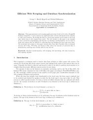
Consider a sampling and reconstruction system as in Figure 1.1. The input signal is x(t) = cos(ω 0 t). The
Fourier transform of the signal is
X(jω) = π [δ(ω − ω 0 ) + δ(ω + ω 0 )]
and the reconstruction (low-pass) filter has the transfer function
{
h, −ωs /2 < ω < ω s /2
F(jω) =
0, else
where ω s = 2π h is the sampling frequency. Find the reconstructed output signal x r(t) for the following input
frequencies
(a) ω 0 = ω s /6
(b) ω 0 = 2ω s /6
(c) ω 0 = 4ω s /6
(d) ω 0 = 5ω s /6
x(t)
p(t)
h
0
t
x(t)
x s (t)
F(jw)
x r (t)
p(t)
Sampling
Reconstruction
0
x s (t)
t
0
t
Figure 1.1: Sampling and reconstruction of a band-limited signal.
EXERCISE 1.2
Let the matrix A be
Compute the matrix exponential e A .
A =
( ) 0 1
.
−1 0
8

EXERCISE 1.3
Compute the z-transform of
x(kh) = e −kh/T T > 0.
EXERCISE 1.4
Compute the z-transform of
x(kh) = sin(wkh)
EXERCISE 1.5
Given the following system described by the following difference equation
y(k + 2) − 1.5y(k + 1) + 0.5y(k) = u(k + 1)
with initial condition y(0) = 0.5 and y(1) = 1.25, determine the output when the input u(k) is a unitary step.
2 Models of sampled systems
EXERCISE 2.1 (Ex. 2.1 in [2])
Consider the scalar system
dx
= −ax + bu
dt
y = cx.
Let the input be constant over periods of length h. Sample the system and discuss how the poles of the discretetime
system vary with the sampling frequency.
EXERCISE 2.2
Consider the following continuous-time transfer function
G(s) =
The system is sampled with sampling period h = 1.
1
(s + 1)(s + 2) .
(a) Derive a state-space representation of the sampled system.
(b) Find the pulse-transfer function corresponding to the system in (a).
9

EXERCISE 2.3 (Ex. 2.2 in [2])
Derive the discrete-time system corresponding to the following continuous-time systems when a zero orderhold
circuit is used
(a)
ẋ =
( ) ( 0 1 0
x + u
−1 0 1)
y = ( 1 0 ) x
(b)
(c)
d 2 y
dt 2 + 3dy du
+ 2y =
dt dt + 3u
d 3 y
dt 3 = u
EXERCISE 2.4 (Ex. 2.3 in [2])
The following difference equations are assumed to describe continuous-time systems sampled using a zeroorder-hold
circuit and the sampling period h. Determine, if possible, the corresponding continuous-time systems.
(a)
(b)
(c)
x(kh + h) =
y(kh) − 0.5y(kh − h) = 6u(kh − h)
( )
−0.5 1
x(kh) +
0 −0.3
y(kh) = ( 1 1 ) x(kh)
y(kh) + 0.5y(kh − h) = 6u(kh − h)
( ) 0.5
u(kh)
0.7
EXERCISE 2.5 (Ex. 2.11 in [2])
The transfer function of a motor can be written as
Determine:
(a) the sampled system
(b) the pulse-transfer function
(c) the pulse response
G(s) =
(d) a difference equation relating input and output
1
s(s + 1) .
(e) the variation of the poles and zeros of the pulse-transfer function with the sampling period
10

EXERCISE 2.6 (Ex. 2.12 in [2])
A continuous-time system with transfer function
G(s) = 1 s e−sτ
is sampled with sampling period h = 1, where τ = 0.5.
(a) Determine a state-space representation of the sampled system. What is the order of the sampled-system?
(b) Determine the pulse-transfer function and the pulse response of the sampled system
(c) Determine the poles and zeros of the sampled system.
EXERCISE 2.7 (Ex. 2.13 in [2])
Solve Problem 2.6 with
and h = 1 and τ = 1.5.
G(s) = 1
s + 1 e−sτ
EXERCISE 2.8 (Ex. 2.15 in [2])
Determine the polynomials A(q), B(q), A ∗ (q −1 )) and B ∗ (q −1 ) so that the systems
A(q)y(k) = B(q)u(k)
and
A ∗ (q −1 )y(k) = B ∗ (q −1 )u(k − d)
represent the system
y(k) − 0.5y(k − 1) = u(k − 9) + 0.2u(k − 10).
What is d? What is the order of the system?
EXERCISE 2.9 (Ex. 2.17 in [2])
Use the z-transform to determine the output sequence of the difference equation
y(k + 2) − 1.5y(k + 1) + 0.5y(k) = u(k + 1)
when u(k) is a step at k = 0 and when y(0) = 0.5 and y(−1) = 1.
11

EXERCISE 2.10
Consider the following continuous time controller
U(s) = − s 0s + s 1
s + r 1
Y (s) + t 0s + t 1
s + r 1
R(s)
where s 0 ,s 1 ,t 0 ,t 1 and r 1 are parameters that are chosen to obtain the desired closed-loop performance. Discretize
the controller using exact sampling by means of sampled control theory. Assume that the sampling
interval is h, and write the sampled controller on the form u(kh) = −H y (q)y(kh) + H r (q)r(kh).
EXERCISE 2.11 (Ex. 2.21 in [2])
If β < α, then
s + β
s + α
is called a lead filter (i.e. it gives a phase advance). Consider the discrete-time system
(a) Determine when it is a lead filter
z + b
z + a
(b) Simulate the step response for different pole and zero locations
3 Analysis of sampled systems
EXERCISE 3.1 (Ex. 3.2 in [2])
Consider the system in Figure 3.1 and let
H(z) =
K
z(z − 0.2)(z − 0.4)
K > 0
Determine the values of K for which the closed-loop system is stable.
r
-
e
H(z)
y
Figure 3.1: Closed-loop system for Problem 3.1.
12

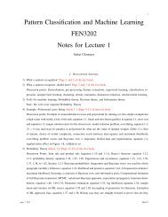
EXERCISE 3.2 (Ex. 3.3 in [2])
Consider the system in Figure 3.2. Assume the sampling is periodic with period h, and that the D-A converter
holds the control signal constant over a sampling interval. The control algorithm is assumed to be
u(kh) = K ( r(kh − τ) − y(kh − τ) )
where K > 0 and τ is the computation time. The transfer function of the process is
G(s) = 1 s .
(a) How large are the values of the regulator gain, K, for which the closed-loop system is stable when τ = 0
and τ = h?
(b) Compare this system with the corresponding continuous-time systems, that is, when there is a continuoustime
proportional controller and a time delay in the process.
H(q)
r u y
C(q)
A/D G(s) D/A
-
Figure 3.2: Closed-loop system for Problem 3.2.
EXERCISE 3.3 (Ex. 3.6 in [2])
Is the following system (a) observable, (b) reachable?
x(k + 1) =
( 0.5 −0.5
0 0.25
y(k) = ( 2 −4 ) x(k)
)
x(k) +
( 6
4)
u(k)
EXERCISE 3.4 (Ex. 3.7 in [2])
Is the following system reachable?
x(k + 1) =
( ) 1 0
x(k) +
0 0.5
( ) 1 1
u(k).
1 0
Assume that a scalar input v(k) such that
u(k) =
( ) 1
v(k)
−1
is introduced. Is the system reachable from v(k)?
13

EXERCISE 3.5 (Ex. 3.11 in [2])
Determine the stability and the stationary value of the output for the system described by Figure 3.2 with
H(q) =
1
q(q − 0.5)
where r is a step function and C(q) = K (proportional controller), K>0.
EXERCISE 3.6 (Ex. 3.12 in [2])
Consider the Problem 3.5. Determine the steady-state error between the reference signal r and the output y,
when r is a unit ramp, that is r(k) = k. Assume C(q) to be a proportional controller.
EXERCISE 3.7 (Ex. 3.18 in [2])
Consider a continuous-time (CT) system
ẋ(t) = Ax(t) + Bu(t)
y(t) = Cx(t).
The zero-order hold sampling of CT gives the discrete-time (DT) system
x(kh + h) = Φx(kh) + Γu(kh)
y(kh) = Cx(kh).
Consider the following statements:
(a) CT stable ⇒ DT stable
(b) CT unstable ⇒ DT unstable
(c) CT controllable ⇒ DT controllable
(d) CT observable ⇒ DT observable.
Which statements are true and which are false (explain why) in the following cases:
(i) For all sampling intervals h > 0
(ii) For all h > 0 except for isolated values
(iii) Neither (i) nor (ii).
EXERCISE 3.8 (Ex. 3.20 in [2])
Given the system
(q 2 + 0.4q)y(k) = u(k),
(a) for which values of K in the proportional controller
u(k) = K ( r(k) − y(k) )
is the closed-loop system stable?
(b) Determine the stationary error r − y when r is a step and K=0.5 in the controller (a).
14

EXERCISE 3.9 (Ex. 4.1 in [2])
A general second-order discrete-time system can be written as
( )
a11 a
x(k + 1) = 12
x(k) +
a 21 a 22
y(k) = ( c 1
Determine a state-feedback controller in the form
c 2
)
x(k).
u(k) = −Lx(k)
such that the characteristic equation of the closed-loop system is
z 2 + p 1 z + p 2 = 0.
(
b1
b 2
)
u(k)
Use the previous result to compute the deadbeat controller for the double integrator.
EXERCISE 3.10 (Ex. 4.2 in [2])
Given the system
x(k + 1) =
( ) ( 1 0.1 1
x(k) + u(k)
0.5 0.1 0)
y(k) = ( 1 1 ) x(k).
Determine a linear state-feedback controller
u(k) = −Lx(k)
such that the poles of the closed-loop system are placed in 0.1 and 0.25.
EXERCISE 3.11 (Ex. 4.5 in [2])
The system
x(k + 1) =
( ) 0.78 0
x(k) +
0.22 1
y(k) = ( 0 1 ) x(k).
( ) 0.22
u(k)
0.03
represents the normalized motor for the sampling interval of h = 0.25. Determine observers for the state based
on the output by using each of the following:
(a) Direct calculation.
(b) An full-state observer.
(c) The reduced-order observer.
15

EXERCISE 3.12 (Ex. 4.8 in [2])
Given the discrete-time system
x(k + 1) =
( ) 0.5 1
x(k) +
0.5 0.7
y(k) = ( 1 0 ) x(k).
( ) ( 0.2 1
u(k) + v(k)
0.1 0)
where v is a constant disturbance. Determine controller such that the influence of v can be eliminated in steady
state in each of the following cases:
(a) The state and v can be measured.
(b) The state can be measured.
(c) Only the output can be measured.
EXERCISE 3.13 (Ex. 4.6 in [2])
Figure 3.13 shows a system with two tanks, where the input signal is the flow to the first tank and the output is
the level of water in the second tank. The continuous-time model of the system is
( ) ( )
−0.0197 1 0.0263
ẋ =
x + u
0.0178 −0.0129 0
y = ( 0 1 ) x.
u
x 1
x 2
Figure 3.13: Closed-loop system for Problem 3.13.
(a) Sample the system with h = 12.
(b) Verify that the pulse-transfer operator for the system is
H(q) =
0.030q + 0.026
q 2 − 1.65q + 0.68
(c) Determine a full-state observer. Choose the gain such that the observer is twice as fast as the open-loop
system.
16

EXERCISE 3.14
Consider the following scalar linear system
ẋ(t) = −5x(t) + u(t)
y(t) = x(t).
(a) Sample the system with sampling period h = 1,
(b) Show, using Lyapunov result, that the sampled system is stable when the input u(kh) = 0 for k ≥ 0.
EXERCISE 3.15
Consider the following linear system
ẋ(t) =
y(t) = x(t).
(a) Sample the system with sampling period h = 1
( ) ( −1 0 1
x(t) + u(t)
0 −2 1)
(b) Design a controller that place the poles in 0.1 and 0.2.
(c) Show, using Lyapunov result, that the closed loop sampled system is stable
4 Computer realization of controllers
EXERCISE 4.1
Consider the following pulse-transfer
H(z) =
z − 1
(z − 0.5)(z − 2)
(a) Design a digital PI controller
H c (z) = (K + K i)z − K
z − 1
that places the poles of the closed-loop system in the origin.
(b) Find a state-space representation of the digital controller in (a).
EXERCISE 4.2 (Ex. 8.2 in [2])
Use different methods to make an approximation of the transfer function
G(s) =
17
a
s + a

(a) Euler’s method
(b) Tustin’s approximation
(c) Tustin’s approximation with pre-warping using ω 1 = a as warping frequency
EXERCISE 4.3 (Ex. 8.3 in [2])
The lead network with transfer function
G l (s) = 4 s + 1
s + 2
Give a phase advance of about 20 ◦ at ω c = 1.6rad/s. Approximate the network for h = 0.25 using
(a) Euler’s method
(b) Backward differences
(c) Tustin’s approximation
(d) Tustin’s approximation with pre-warping using ω 1 = ω c as warping frequency
EXERCISE 4.4 (Ex. 8.7 in [2])
Consider the tank system in Problem 2.13. Assume the following specifications:
1. The steady-state error after a step in the reference value is zero
2. The crossover frequency of the compensated system is 0.025 rad/s
3. The phase margin is about 50 ◦ .
(a) Design a PI-controller such that the specifications are fulfilled.
(b) Determine the poles and the zeros of the closed-loop system. What is the damping corresponding to the
complex poles?
(c) Choose a suitable sampling interval and approximate the continuous-time controller using Tustin’s method
with pre-warping. Use the crossover frequency as warping frequency.
EXERCISE 4.5 (Ex. 8.4 in [2])
The choice of sampling period depends on many factors. One way to determine the sampling frequency is to use
continuous-time arguments. Approximate the sampled system as the hold circuit followed by the continuoustime
system. Assuming that the phase margin can be decreased by 5 ◦ to 15 ◦ , verify that a rule of thumb in
selecting the sampling frequency is
hω c ≈ 0.15 to 0.5
where ω c is the crossover frequency of the continuous-time system.
18

EXERCISE 4.6 (Ex. 8.12 in [2])
Consider the continuous-time double integrator described by
( ) ( 0 1 0
ẋ = x + u
0 0 1)
y = ( 1 0 ) x.
Assume that a time-continuous design has been made giving the controller
with K T = (1,1).
u(t) = 2r(t) − ( 12 ) ˆx(t)
dˆx(t)
dt
= Aˆx(t) + Bu(t) + K ( y(t) − Cˆx(t) )
(a) Assume that the controller should be implemented using a computer. Modify the controller (not the
observer part) for the sampling interval h = 0.2 using the approximation for state models.
(b) Approximate the observer using a backward-difference approximation
EXERCISE 4.7
Consider the following continuous time controller
U(s) = − s 0s + s 1
s + r 1
Y (s) + t 0s + t 1
s + r 1
R(s)
where s 0 ,s 1 ,t 0 ,t 1 and r 1 are parameters that are chosen to obtain the desired closed-loop performance.
(a) Discretize the controller using forward difference approximation. Assume that the sampling interval is
h, and write the sampled controller on the form u(kh) = −H y (q)y(kh) + H r (q)r(kh).
(b) Assume the following numerical values of the coefficients: r 1 = 10, s 0 = 1, s 1 = 2, t 0 = 0.5 and
t 1 = 10. Compare the discretizations obtained in part (a) for the sampling intervals h = 0.01, h = 0.1
and h = 1. Which of those sampling intervals should be used for the forward difference approximation?
EXERCISE 4.8
Consider the following continuous-time controller in state-space form
ẋ = Ax + Be
u = Cx + De
(a) Derive the backward-difference approximation in state-space form of the controller, i.e. derive Φ c , Γ c ,
H and J for a system
w(k + 1) = Φ c w(k) + Γ c e(k)
u(k) = Hw(k) + Je(k)
19

(b) Prove that the Tustin’s approximation of the controller is given by
Φ c =
Γ c =
(
I + A ch
2
(
I − A ch
2
H = C c
(
I − A ch
2
) (
I − A ch
2
) −1
B c h
2
) −1
J = D c + C c
(
I − A ch
2
) −1
) −1
B c h
2 .
5 Implementation aspects
EXERCISE 5.1
Consider the discrete-time controller characterized by the pulse-transfer function
H(z) =
Implement the controller in parallel form.
1
(z − 1)(z − 1/2)(z 2 + 1/2z + 1/4) .
EXERCISE 5.2
(a) Given the system in Figure 5.2, find the controller C s (s) such that the closed loop transfer function from
r to y becomes
H cl =
C(s)P(s)
1 + C(s)P(s) e−sτ
(b) Let
find the expression for the Smith predictor C s (s).
P(s) = 1
s + 1
8
H cl (s) =
s 2 + 4s + 8 e−sτ
r(t)
__
C s (s) e −sτ P(s)
y(t)
Figure 5.2: System of Problem 5.2.
20

EXERCISE 5.3
A process with transfer function
is controlled by the PI-controller
P(z) =
z
z − 0.5
z
C(z) = K p + K i
z − 1
where K p = 0.2 and K i = 0.1. The control is performed over a wireless network, as shown in Figure 5.3. Due
to retransmission of dropped packets, the network induces time-varying delays. How large can the maximum
delay be, so that the closed loop system is stable?
P(z)
ZOH
G(s)
Sample
Wireless Network
C(z)
Figure 5.3: Closed loop system for Problem 5.3.
EXERCISE 5.4 (Inspired by Ex. 9.15 in [2])
Two different algorithms for a PI-controller are listed. Use the linear model for roundoff to analyze the sensitivity
of the algorithms to roundoff in multiplications and divisions. Assume that the multiplications happen in
the order as they appear in the formula and that they are executed before the division.
Algorithm 1:
repeat
e:=r-y
u:=k*(e+i)
i:=i+e*h/ti
forever
21

Algorithm 2:
repeat
e:=r-y
u:=i+k*e
i:=k*i+k*h*e/ti
forever
EXERCISE 5.5
Consider a first-order system with the discrete transfer function
H(z) =
1
1 − az −1 a = 1 8 .
Assume the controller is implemented using fixed point arithmetic with 8 bits word length and h = 1 second.
Determine the system’s unit step response for sufficient number of samples to reach steady-state. Assume that
the data representation consists of
• 1 bit for sign
• 2 bits for the integer part
• 5 bits for the fraction part
and consider the cases of truncation and round-off.
22

Part II
Event-triggered control
23

6 Real-time operating systems
EXERCISE 6.1
In an embedded control system the control algorithm is implemented as a task in a CPU. The control task J c
can compute the new control action only after the acquisition task J a has acquired new sensor measurements.
The two tasks are independent and they share the same CPU. Suppose the sampling period is h = 0.4 seconds
and the tasks have the following specifications
C i
J c 0.1
J a 0.2
We assume that the period T i and the deadline D i are the same for the two tasks, and the release time is 0 for
both tasks.
(a) Is possible to schedule the two tasks J c and J a ? Determine the schedule length and draw the schedule.
(b) Suppose that a third task is running in the CPU. The specifications for the task are
C i T i = D i r i
J x 0.2 0.8 0.3
and we assume that the task J x has higher priority than the tasks J c and J a . We also assume the CPU can
handle preemption. Are the three tasks schedulable? Draw the schedule and determine the worst-case response
time for the control task J c .
EXERCISE 6.2
A digital PID controller is used to control the plant, which sampled with period h = 2 has the following transfer
function
P(z) = 1 z − 0.1
100 z − 0.5 .
The control law is
(
C(z) = 15 1 + z )
.
z − 1
Assume that the control task J c is implemented on a computer and has C c = 1 as the worst case computation
time. Assume that a higher priority interrupt occurs at time t = 2 which has a worst case computation time C I .
Determine the largest value of C I such that the closed loop system is stable.
EXERCISE 6.3
A robot has been designed with three different tasks J A , J B , J C , with increasing priority. The task J A is a low
priority thread which implements the DC-motor controller, the task J B periodically send a "ping" through the
wireless network card so that it is possible to know if the system is running. Finally the task J C , with highest
priority, is responsible to check the status of the data bus between two I/O ports, as shown in Figure 6.3. The
control task is at low priority since the robot is moving very slowly in a cluttered environment. Since the data
bus is a shared resource there is a semaphore that regulates the access to the bus. The tasks have the following
characteristics
24

T i
C i
J A 8 4
J B 5 2
J C 1 0.1
Assuming the kernel can handle preemption, analyze the following possible working condition:
• at time t = 0, the task J A is running and acquires the bus in order to send a new control input to the
DC-motors,
• at time t = 2 the task J C needs to access the bus meanwhile the control task J A is setting the new control
signal,
• at the same t J B is ready to be executed to send the "ping" signal.
(a) Show graphically which tasks are running. What happens to the high priority task J C ? Compute the
response time of J C in this situation.
(b) Suggest a possible way to overcome the problem in (a).
DC-Motors
I/O
Data Bus
I/O
Ping
Dedicated Data Bus
Network Card
CPU
Figure 6.3: Schedule for the control task J c and the task handling the interrupt, of Problem 6.2.
EXERCISE 6.4 (Jackson’s algorithm, page 52 in [3])
We consider here the Jackson’s algorithm to schedule a set J of n aperiodic tasks minimizing a quantity called
maximum lateness and defined as
( )
L max := max fi − d i .
i∈J
All the tasks consist of a single job, have synchronous arrival times but have different computation times and
deadlines. They are assumed to be independent. Each task can be characterized by two parameters, deadline d i
and computation time C i
J = {J i |J i = J i (C i ,d i ), i = 1,... ,n}.
The algorithm, also called Earliest Due Date (EDD), can be expressed by the following rule
25

Theorem 1. Given a set of n independent tasks, any algorithm that executes the tasks in order of nondecreasing
deadlines is optimal with respect to minimizing the maximum lateness.
(a) Consider a set of 5 independent tasks simultaneously activated at time t = 0. The parameters are indicated
in the following table
J 1 J 2 J 3 J 4 J 5
C i 1 1 1 3 2
d i 3 10 7 8 5
Determine what is the maximum lateness using the scheduling algorithm EDD.
(b) Prove the optimality of the algorithm.
7 Real-time scheduling
EXERCISE 7.1 (Ex. 4.3 in [3])
Verify the schedulability and construct the schedule according to the rate monotonic algorithm for the following
set of periodic tasks
C i
T i
J 1 1 4
J 2 2 6
J 3 3 10
EXERCISE 7.2 (Ex. 4.4 in [3])
Verify the schedulability under EDF of the task set given in Exercise 7.1 and then construct the corresponding
schedule.
EXERCISE 7.3
Consider the following set of tasks
C i T i D i
J 1 1 3 3
J 2 2 4 4
J 3 1 7 7
Are the tasks schedulable with rate monotonic algorithm? Are the tasks schedulable with earliest deadline first
algorithm?
26

EXERCISE 7.4
Consider the following set of tasks
C i T i D i
J 1 1 4 4
J 2 2 5 5
J 3 3 10 10
Assume that task J 1 is a control task. Every time that a measurement is acquired, task J 1 is released. When
executing, it computes an updated control signal and outputs it.
(a) Which scheduling of RM or EDF is preferable if we want to minimize the delay between the acquisition
and control output?
(b) Suppose that J 2 is also a control task and that we want its maximum delay between acquisition and
control output to be two time steps. Suggest a schedule which guarantees a delay of maximally two time
steps, and prove that all tasks will meet their deadlines.
EXERCISE 7.5
Consider the two tasks J 1 and J 2 with computation times, periods and deadlines as defined by the following
table:
C i T i D i
J 1 1 3 3
J 2 1 4 4
(a) Suppose the tasks are scheduled using the rate monotonic algorithm. Will J 1 and J 2 meet their deadlines
according to the schedulability condition on the utilization factor? What is the schedule length, i.e., the
shortest time interval that is necessary to consider in order to describe the whole time evolution of the
scheduler? Plot the time evolution of the scheduler when the release time for both tasks is at t = 0.
(b) If the two tasks implement a controller it is important to know what is the worst-case delay between the
time the controller is ready to sample and the time a new input u(kh) is ready to be released. Find the
worst-case response time for J 1 and J 2 . Compare with the result in (a).
EXERCISE 7.6
Consider the set of periodic tasks given in the table below:
C i T i O i
J 1 1 3 1
J 2 2 5 1
J 3 1 6 0
where for task i, C i the worst-case execution time, T i denotes the period, and O i the offset for the respective
tasks. Assume that the deadlines coincide with the period. The offset denotes the relative release time of the
first task instance for each task. Assume that all tasks are released at time 0 with their respective offset O i .
27

(a) Determine the schedule length.
Determine the worst-case response time for task J 2 for each of the following three scheduling policies:
(b) Rate-monotonic scheduling
(c) Deadline-monotonic scheduling
(d) Earliest-deadline-first scheduling
EXERCISE 7.7
A control task J c is scheduled in a computer together with two other tasks J 1 and J 2 . Assume that the three
tasks are scheduled using a rate monotonic algorithm. Assume that the release time for all tasks are at zero and
that the tasks have the following characteristics
C i T i D i
J 1 1 4 4
J 2 1 6 6
J c 2 5 5
(a) Is the set of tasks schedulable with rate monotonic scheduling? Determine the worst-case response time
for the control task J c .
(b) Suppose the control task implements a sampled version of the continuous-time controller with delay
ẋ(t) = Ax(t) + By(t − τ)
u(t) = Cx(t)
where we let τ be the worst-case response time R c of the task J c . Suppose that the sampling period of the
controller is h = 2 and R c = 3. Derive a state-space representation for the sampled controller. Suggest
also an implementation of the controller by specifying a few lines of computer code.
(c) In order to improve performance the rate monotonic scheduling is substituted by a new scheduling algorithm
that give highest priority to the control task and intermediate and lowest to the task J 1 and J 2 ,
respectively. Are the tasks schedulable in this case?
EXERCISE 7.8
Compute the maximum processor utilization that can be assigned to a polling server to guarantee the following
periodic task will meet their deadlines
C i
T i
J 1 1 5
J 2 2 8
28

EXERCISE 7.9
Together with the periodic tasks
C i
T i
J 1 1 4
J 2 1 8
we want to schedule the following aperiodic tasks with a polling server having T s = 5 and C s = 2. The
aperiodic tasks are
a i
C i
a 1 2 3
a 2 7 2
a 3 9 1
a 3 29 4
EXERCISE 7.10
Consider the set of tasks in Problem 7.5, assuming that an aperiodic task could ask for CPU time. In order
to handle the aperiodic task we run a polling server J s with computation time C s = 3 and period T s = 6.
Assume that the aperiodic task has computation time C a = 3 and asks for the CPU at time t = 3. Plot the time
evolution when a polling server is used together with the two tasks J 1 and J 2 scheduled as in Problem 7.5 part
(a). Describe the scheduling activity illustrated in the plots.
8 Models of computation I: Discrete-event systems
EXERCISE 8.1
Consider the problem of controlling a gate which is lowered when a train is approaching and it is raised when
the train has passed. We assume that the railway is unidirectional and that a train can be detected 1500m before
the gate and 1000m after the gate. The sensors give binary outputs i.e., they give a ’0’ when the train is not over
the sensor and a ’1’ when the train is over the sensor. The gate has a sensor which gives a binary information
and in particular gives ’0’ if the gate is (fully) closed and ’1’ if the gate is (fully) opened. Figure 8.1 shows
a schema of the system. The gate needs to be lowered as soon as a train is approaching, and raised when the
train has passed. Model the system as a discrete-event system. Assume that trains, for safety reasons are distant
from each other, so that no train approaches before the previous train has left.
EXERCISE 8.2
A vending machine dispenses soda for $0.45. It accepts only dimes ($0.10) and quarters ($0.25). It does not
give change in return if your money is not correct. The soda is dispensed only if the exact amount of money
is inserted. Model the vending machine using a discrete-event system. Is it possible that the machine does not
dispense soda? Prove it formally.
29

1000m
1500m
Gate
Train
S 3
A
S 2
S 1
Controller
Figure 8.1: Control of a gate. Problem 8.1.
EXERCISE 8.3
Consider the automaton describing some discrete-event system shown in Figure 8.3. Describe formally the
0
q 1 q 2
Figure 8.3: Automaton A of Problem 8.3.
DES. Compute the marked language L m and the generated language L.
1
EXERCISE 8.4 (Example 2.13 in [5])
Consider the automaton A of Figure 8.4. Compute the language marked by the automaton A, L m (A) and the
language generated by the automaton, L(A).
1
0 1
q 1 q 2 q 3
0
0,1
Figure 8.4: Automaton A of Problem 8.4.
30

EXERCISE 8.5 (Example 3.8 in [5])
Consider the automaton A of Figure 8.5. Determine the minimum state automaton.
1
a
0
0 1
b
0
1
c
0
1
d
0
e
1
f
1
g
0
1
h
1
0
0
Figure 8.5: Automaton A of Problem 8.5.
EXERCISE 8.6 (Example 2.5 in [5])
Consider the automaton
A = ({q 0 ,q 1 }, {0,1},δ,q 0 , {q 1 })
be a nondeterministic automaton where
δ(q 0 ,0) = {q 0 ,q 1 } δ(q 0 ,1) = {q 1 } δ(q 1 ,0) = δ(q 1 ,1) = {q 0 ,q 1 }.
Construct an deterministic automaton A ′ which accept the same L m .
9 Models of computation II: Transition systems
EXERCISE 9.1
Consider a Discrete Event System described by an automaton and model it formally as a transition system.
EXERCISE 9.2
Try to model by a transition system the basic functionalities of the keypad of a mobile phone, including the
states mainmenu, contacts and lock.
EXERCISE 9.3 [4]
31

Queuing systems arises in many application domain such as computer networks, manufacturing, logistics and
transportation. A queuing systems is composed by three basic elements: 1) the entities, generally referred to
as customers, that do the waiting in their request for resources, 2) the resources for which the waiting is done,
which are referred to as servers, and 3) the space where the waiting is done, which is defined as queue. Typical
examples of servers are communications channels, which have a finite capacity to transmit information. In
such a case, the customers are the unit of information and the queue is the amount of unit of information that is
waiting to be transmitted over the channel.
A basic queue system is reported in figure 9.3. The circle represent a server, the open box is a queue
preceding the server. The slots in the queue are waiting customers. The arrival rate of customers in the queue
is denoted by a, whereas the departure rate of customers is denoted by b.
Model the queue system of figure 9.3 by a transition system. How many states has the system?
queue
server
C ustom ers
A rrivals
C ustom ers
D eparture
Figure 9.3: A basic queue system.
EXERCISE 9.4 [14]
Consider the transition system T = {S,Σ, →,S S }, where the cardinality of S is finite. The reachability
algorithm is
Initialization : Reach 1 = ∅;
Prove formally that
Reach 0 = S S ;
i = 0;
Loop : While Reach i ≠ Reach i−1 do
Reach i+1 = Reach i ∪ {s ′ ∈ S : ∃ : s ∈ Reach i ,σ ∈ Σ,s → σ s ′ ∈→};
i = i + 1;
• the reachability algorithm finishes in a finite number of steps;
• upon exiting the algorithm, Reach i = Reach T (S S ).
EXERCISE 9.5 [14]
Give the Transition System T = {S,Σ, →,S S } reported in figure 9.5, describe the reach set when S S = {3}
and S S = {2} by using the teachability algorithm.
32

1
a b a
2 3
a a a b
4 5 6
Figure 9.5: A Transition System.
33

Part III
Hybrid control
34

10 Modeling of hybrid systems
EXERCISE 10.1
A water level in a tank is controlled through a relay controller, which senses continuously the water level and
turns a pump on or off. When the pump is off the water level decreases by 2 cm/s and when it is on, the water
level increases by 1 cm/s. It takes 2 s for the control signal to reach the pump. It is required to keep the water
level between 5 and 12 cm.
(a) Assuming that the controller starts the pump when the level reaches some threshold and turns it of when
it reaches some other threshold, model the closed-loop system as a hybrid automaton.
(b) What thresholds should be used to fulfill the specifications?
EXERCISE 10.2
Consider the quantized control system in Figure 10.2. Such a system can be modeled as a hybrid automaton
with continuous dynamics corresponding to P(s)C(s) and discrete states corresponding to the levels of the
quantizer. Suppose that each level of the quantizer can be encoded by a binary word of k bits. Then, how
many discrete states N should the hybrid automaton have? Describe when discrete transitions in the hybrid
automaton should take place.
v
P(s)
v = Q(u)
u
Q
C(s)
D
D
2
u
Figure 10.2: Quantized system in Problem 10.2.
EXERCISE 10.3
A system to cool a nuclear reactor is composed by two independently moving rods. Initially the coolant temperature
x is 510 degrees and both rods are outside the reactor core. The temperature inside the reactor increases
according to the following (linearized) system
ẋ = 0.1x − 50.
When the temperature reaches 550 degrees the reactor mush be cooled down using the rods. Three things can
happen
• the first rod is put into the reactor core
• the second rod is put into the reactor core
• none of the rods can be put into the reactor
35

For mechanical reasons a rod can be placed in the core if it has not been there for at least 20 seconds. If no
rod is available the reactor should be shut down. The two rods can refrigerate the coolant according to the two
following ODEs
rod 1: ẋ = 0.1x − 56
rod 2: ẋ = 0.1x − 60
When the temperature is decreased to 510 degrees the rods are removed from the reactor core. Model the
system, including controller, as a hybrid system.
Rod 2
Rod 1
Controller
Reactor
Figure 10.3: Nuclear reactor core with the two control rods
EXERCISE 10.4
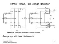
Consider the classical sampled control system, shown in Figure 10.4. Model the system with a hybrid automaton.
Suppose that the sampling period is k and that the hold circuit is a zero-order hold.
EXERCISE 10.5
Consider a hybrid system with two discrete states q 1 and q 2 . In state q 1 the dynamics are described by the linear
system
( ) −1 0
ẋ = A 1 x =
p −1
and in state q 2 by
Assume the system is
ẋ = A 2 x =
( ) −1 p
.
0 −1
36

u(t)
y(t)
t
u(t)
y(t)
Process
Hold
Sample
u k ū k ȳ k y k
DA Computer AD
u k
...
...
t
Figure 10.4: Sampled data control system of Problem 10.4.
y k
.......
t
t
in state q 1 if 2k ≤ t < 2k + 1 and
in state q 2 if 2k + 1 ≤ t < 2k + 2,
where k = 0,1,2,... .
(a) Formally define a hybrid system with initial state q 1 , which operates in the way described above.
(b) Starting from x(0) = x 0 , specify the evolution of the state x(t) in the interval t ∈ [0,3) as a function of
x 0 .
EXERCISE 10.6
Consider the hybrid system of Figure 10.6:
(a) Describe it as a hybrid automaton, H = (Q,X, Init,f,D,E,G,R)
(b) Find all the domains D(q 3 ) so that the hybrid system is live?
(c) Plot the solution of the hybrid system.
x(0) := 0
q 1
x ≥ 5
q 2
x ≤ 3, x := −2
q 3
ẋ = 2
ẋ = −1
ẋ = x + 2
x < 5
x > 3
D(q 3 ) =?
Figure 10.6: Hybrid system for Problem 10.6.
37

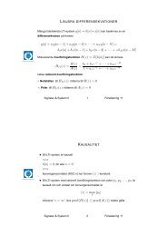
11 Stability of hybrid systems
EXERCISE 11.1
Consider three balls with unit mass, velocities v 1 , v 2 , v 3 , and suppose that they are touching at time t = τ 0 , see
Figure 11.1. The initial velocity of Ball 1 is v 1 (τ 0 ) = 1 and Balls 2 and 3 are at rest, i.e., v 2 (τ 0 ) = v 3 (τ 0 ) = 0.
v 1
Ball 1 Ball 2 Ball 3
Figure 11.1: Three balls system. The Ball 1 has velocity v 1 at time t = 0.
Assume that the impact is a sequence of simple inelastic impacts occurring at τ 0 ′ = τ 1 ′ = τ 2 ′ = ... (using
notation from hybrid time trajectory). The first inelastic collision occurs at τ 0 ′ between balls 1 and 2, resulting
in v 1 (τ 1 ) = v 2 (τ 1 ) = 1/2 and v 3 (τ 1 ) = 0. Since v 2 (τ 1 ′) > v 3(τ 1 ′ ), Ball 2 hits Ball 3 instantaneously giving
v 1 (τ 2 ) = 1/2, and v 2 (τ 2 ) = v 3 (τ 2 ) = 1/4. Now v 1 (τ 2 ′) > v 2(τ 2 ′ ), so Ball 1 hits Ball 2 again resulting in a new
inelastic collision. This leads to an infinite sequence of collisions.
(a) Model the inelastic collisions of the three-ball system described above as a hybrid automaton H =
(Q,X, Init,f,D,E,G,R) with one discrete variable Q = {q} and three continuous variables X =
{v 1 ,v 2 ,v 3 }.
(b) Is the execution described above a Zeno execution? Motivate.
(c) What is the accumulation point of the infinite series of hits described above? Make a physical interpretation.
EXERCISE 11.2
Consider the following system
⎛ ⎞ ⎛ ⎞ ⎛ ⎞
ẋ 1 −1 0 2 x 1
⎝ẋ 2
⎠ = ⎝ 0 −1 3 ⎠ ⎝x 2
⎠
ẋ 3 −2 −3 −2 x 3
Show, using a Lyapunov function, that the system is asymptotically stable.
EXERCISE 11.3
Consider the following theorem:
Theorem 2. A linear system
ẋ = Ax
is asymptotically stable if and only if for any positive definite symmetric matrix Q the equation
A T P + PA = −Q
in the unknown P ∈ R n×n has a solution which is positive definite and symmetric.
Show the necessary part of the previous theorem (i.e., the if part).
38

EXERCISE 11.4
Consider the following system
ẋ 1 = −x 1 + g(x 2 )
ẋ 2 = −x 2 + h(x 1 )
where the functions g and h are such that
|g(z)| ≤ |z|/2
|h(z)| ≤ |z|/2
Show that the system is asymptotically stable.
EXERCISE 11.5
Consider the following discontinuous differential equations
ẋ 1 = −sgn(x 1 ) + 2sgn(x 2 )
ẋ 2 = −2sgn(x 1 ) − sgn(x 2 ).
where
sgn(z) =
{
+1 if z ≥ 0
−1 if z < 0.
Assume x(0) ≠ 0,
(a) define a hybrid automaton that models the discontinuous system
(b) does the hybrid automaton exhibit Zeno executions for every initial state?
EXERCISE 11.6
Consider the following switching system
ẋ = a q x, a q < 0 ∀q
where q ∈ {1,2} and
Ω 1 = {x ∈ R|x ∈ [2k,2k + 1),k = 0,1,2,... }
Ω 2 = {x ∈ R|x ∈ [2k + 1,2k + 2),k = 0,1,2,... }
Show that the system is asymptotically stable.
39

EXERCISE 11.7
Consider the following switching system
where q ∈ {1,2} and
ẋ = A q x
( ) −1 0
A 1 =
0 −2
( ) −3 0
A 2 = .
0 −5
Let Ω q be such that
Show that the system is asymptotically stable.
Ω 1 = {x ∈ R 2 |x 1 ≥ 0}
Ω 2 = {x ∈ R 2 |x 1 < 0}
EXERCISE 11.8
Consider the following switching system
where q ∈ {1,2} and
ẋ = A q x
( )
−a1 b
A 1 = 1
0 −c 1
( )
−a2 b
A 2 = 2
.
0 −c 2
Assume that a i , b i and c i , i = 1,2 are real numbers and that a i ,c i > 0. Show that the switched system is
asymptotically stable.
EXERCISE 11.9
Consider a system that follows the dynamics
for a time ǫ/2 and then switches to the system
ẋ = A 1 x
ẋ = A 2 x
for a time ǫ/2. It then switches back to the first system, and so on.
(a) Model the system as a switched system
(b) Model the system as a hybrid automaton
(c) Let t 0 be a time instance at which the system begins a period in mode 1 (the first system) with initial
condition x 0 . Determine the state at t 0 + ǫ/2 and t 0 + ǫ.
(d) Let ǫ tend to zero (very fast switching). Determine the solution the hybrid system will tend to.
40

EXERCISE 11.10
Consider the following hybrid system
where
ẋ = A q x
( ) −1 0
A 1 =
0 −2
( ) −3 0
A 2 = .
0 −5
Let Ω q be such that
Ω 1 = {x ∈ R 2 |x 1 ≥ 0}
Ω 2 = {x ∈ R 2 |x 1 < 0}
show that the switched system is asymptotically stable using a common Lyapunov function.
EXERCISE 11.11 (Example 2.1.5 page 18-19 in [12])
Consider the following switched system with q ∈ {1,2}
ẋ = A q x
where
( ) −1 −1
A 1 =
1 −1
( ) −1 −10
A 2 = .
0.1 −1
(a) Show that is impossible to find a quadratic common Lyapunov function.
(b) Show that the origin is asymptotically stable for any switching sequence.
EXERCISE 11.12
Consider the following two-dimensional state-dependent switched system
{
A 1 x if x 1 ≤ 0
ẋ =
A 2 x if x 1 > 0
where
A 1 =
( ) −5 −4
−1 −2
and A 2 =
( ) −2 −4
.
20 −2
(a) Prove that there is not a common quadratic Lyapunov function suitable to prove stability of the system
(b) Prove that the switched system is asymptotically stable using the multiple Lyapunov approach.
41

12 Verification of hybrid systems
EXERCISE 12.1
Consider the following linear system
ẋ =
( ) −1 0
x
0 −5
Assume that the initial condition is defined in the following set
x 0 ∈ {(x 1 ,x 2 ) ∈ R 2 |x 1 = x 2 , −10 ≤ x 1 ≤ 10}
We want to verify that no trajectories enter in a Bad set defined as
Bad = {(x 1 ,x 2 ) ∈ R| − 8 ≤ x 1 ≤ 0 ∧ 2 ≤ x 2 ≤ 6}.
EXERCISE 12.2
Consider the following linear system
ẋ =
Assume that the initial condition lies in the following set
( ) −5 −5
x.
0 −1
x 0 ∈ {(x 1 ,x 2 ) ∈ R 2 | − 2 ≤ x 1 ≤ 0 ∧ 2 ≤ x 2 ≤ 3}.
Describe the system as a transition system and verify that no trajectories enter a Bad set defined as the triangle
with vertices v 1 = (−3,2), v 2 = (−3, −3) and v 3 = (−1,0).
EXERCISE 12.3
Consider the following controlled switched system
⎛
) (ẋ1
= ⎝ 0 1
⎞
( )
1 ⎠ x1
ẋ 2
3 5 + B
x 1 u if ‖x‖ < 1
2
⎛
) (ẋ1
= ⎝ 0 1
⎞
) (
1 ⎠(
x1 0
ẋ 2
3 −1 + u if 1 ≤ ‖x‖ ≤ 3
x 2 1)
⎛⎛
3
) (ẋ1
= − ⎝⎝ 0 1
⎞
⎞
( ) (
1 ⎠ x1 − 1 0
ẋ 2
3 5 + u⎠
otherwise
x 2 1)
Assume that the initial conditions are x 0 ∈ {x ∈ R 2 |‖x‖ > 3},
(a) Determine a control strategy such that Reach q ∪Ω 1 ≠ ∅, i.e. Ω 1 can be reached from any initial condition
when B 1 = 0.
Suppose in the following B 1 = (0,1) T ,
(b) Is it possible to determine a linear control input such that (0,0) is globally asymptotically stable?
(c) Construct a piecewise linear system such that (0,0) is globally asymptotically stable.
(d) Suppose now, that we do not want that the solution of the linear system would enter the Bad set Ω 1 .
Determine a controller such that Reach q ∩ Ω 1 = ∅.
42

EXERCISE 12.4
A system to cool a nuclear reactor is composed by two independently moving rods. Initially the coolant temperature
x is 510 degrees and both rods are outside the reactor core. The temperature inside the reactor increases
accordingly to the following (linearized) system
ẋ = 0.1x − 50.
When the temperature reaches 550 degrees the reactor mush be cool down using the rods. Three things can
happen
• the first rod is put into the reactor core
• the second rod is put into the reactor core
• none of the rods can be put into the reactor
For mechanical reasons the rods can be placed in the core if it has not been there for at least 20 seconds. The
two rods can refrigerate the coolant accordingly to the two following ODEs
rod 1: ẋ = 0.1x − 56
rod 2: ẋ = 0.1x − 60
When the temperature is decreased to 510 degrees the rods are removed from the reactor core.
a Model the system as a hybrid system.
b If the temperature goes above 550 degrees, but there is no rod available to put down in the reactor, there
will be a meltdown. Determine if this Bad state can be reached.
Rod 2
Rod 1
Controller
Reactor
Figure 12.4: Nuclear reactor core with the two control rods
43

a
q 0
a
a
a
q 1
q2
c
c
b
q 3 q 4 q 5 q 6
Figure 13.1: The transition system T .
13 Simulation and bisimulation
EXERCISE 13.1
Figure 13.1 shows a transition system T = {S,Σ, →,S 0 ,S F }, where
S = {q 0 ,...,q 6 }
Σ = {a,b,c}
→ : According to the figure
S 0 = {q 0 }
S F = {q 3 ,q 6 }.
Find the simplest quotient transition system ˆT that is bisimular to T .
EXERCISE 13.2
Here we should insert a problem that the students do themselves: Show a system T and three candidates ˆT i .
Determine which systems are bisimular to T .
44

Solutions
45

Part I
Time-triggered control
46

Solutions to review exercises
SOLUTION 1.1
Before solving the exercise we review some concepts on sampling and aliasing
Shannon sampling theorem
Let x(t) be band-limited signal that is, X(jω) = 0 for |ω| > ω m . Then x(t) is uniquely determined by its
samples x(kh), k = 0, ±1, ±2,... if
ω s > 2ω m
where ω s = 2π/h is the sampling frequency, h the sampling period. The frequency w s /2 is called the Nyquist
frequency.
Reconstruction
Let x(t) be the signal to be sampled. The sampled signal x s (t) is obtained multiplying the input signal x(t) by
a period impulse train signal p(t), see Figure1.1. We have that
Thus the sampled signal is
x s (t) = x(t)p(t)
∞∑
p(t) = δ(t − kh).
x s (t) =
k=−∞
∞∑
k=−∞
x(kh)δ(t − kh).
If we let the signal x s (t) pass through an ideal low-pass filter (see Figure 1.1.1) with impulse response
( ws
)
f(t) = sinc
2 t
and frequency response
{ h, −ωs /2 < ω < ω
F(jω) =
s /2;
o, otherwise.
as shown in Figure 1.1.1. The output signal is
∫ ∞
x r (t) = x s (t) ∗ f(t) = x s (t − τ)f(τ)dτ
−∞
∫ (
∞ ∑ ∞
)
= x(kh)δ(t − τ − kh) f(τ)dτ
=
=
−∞
∞∑
k=−∞
∞∑
k=−∞
k=−∞
x(kh)sinc
( ωs
2 (t − kh) )
( π
)
x(kh)sinc
h (t − kh) .
Notice that perfect reconstruction requires an infinite number of samples.
Returning to the solution of the exercise we have that the Fourier transform of the sampled signal is given
by
X s (ω) = 1 ∞∑
X(ω + kω s )
h
k=−∞
(a) The reconstructed signal is x r (t) = cos(ω 0 t) since ω s = 6ω 0 > 2ω 0 .
47

f(t)
F(jw)
−ω s /2) ω s /2
Figure 1.1.1: Impulse and frequency response of an ideal low-pass filter.
X s (t)
ω 0 − ω s
−ω 0 + ω s
ω
−ω 0
ω 0
−ω0 − ω
ω
−ω s
ω 0 + ω s
s s
Figure 1.1.2: Frequency response of the signal with ω 0 = ω s /6
(b) The reconstructed signal is x r (t) = cos(ω 0 t) since ω s = 6ω 0 /2 > 2ω 0 .
X s (t)
ω 0 − ω s
−ω 0 + ω s
ω
−ω 0
ω 0
−ω0 − ω
ω
−ω s
ω 0 + ω s
s s
Figure 1.1.3: Frequency response of the signal with ω 0 = 6ω s /2
(c) The reconstructed signal is x r (t) = cos ( (−ω 0 + ω s )t ) = cos(ω 0 /2t) since ω s = 6ω 0 /4 < 2ω 0 .
(d) The reconstructed signal is x r (t) = cos ( (−ω 0 + ω s )t ) = cos(ω 0 /5t) since ω s = 6ω 0 /5 < 2ω 0 .
48

X s (t)
ω 0 − ω s
−ω 0 + ω s
ω 0 + ω s
−ω s
−ω 0 ω 0
ω s
ω
−ω0 − ω s
Figure 1.1.4: Frequency response of the signal with ω 0 = 6ω s /4
X s (t)
ω 0 + ω s
ω 0 − ω s
−ω 0 −ω 0 + ω s
ω 0
−ω s
ω s
ω
−ω 0 − ω s
Figure 1.1.5: Frequency response of the signal with ω 0 = 6ω s /5
49

SOLUTION 1.2
We have that
The eigenvalues of Ah are ±ih thus we need to solve
This gives
Thus
e Ah = sin h
h
e Ah = α 0 Ah + Iα 1 .
e ih = α 0 ih + α 1
e −ih = −α 0 ih + α 1 .
α 0 = eih − e −ih
2ih
α 1 = eih + e −ih
2
= sinh
h
= cos h.
( ) ( )
0 1 1 0
h + cos h
−1 0 0 1
We remind here some useful way of computing the matrix exponential of a matrix A ∈ R n×n . Depending
on the form of the matrix A we can compute the exponential in different ways
• If A is diagonal then
⎛
⎞ ⎛
a 11 0 ... 0
e a ⎞
11
0 ... 0
0 a 22 ... 0
A = ⎜
⎝
.
. . ..
⎟
. ⎠ ⇒ 0 e a 22
... 0
eA = ⎜
⎝
.
. . ..
⎟
. ⎠
0 0 ... a nn 0 0 ... e ann
• A is nilpotent of order m. Then A m = 0 and A m+i = 0 for i = 1,2,... . Then it is possible to use the
following series expansion to calculate the exponential
• Using the inverse Laplace transform we have
e A = I + A + A2
2! + · · · + Am−1
(m − 1)!
e At = L −1 ( (sI − A) −1)
• In general it is possible to compute the exponential of a matrix (or any continuous matrix function f(A)))
using the Cayley-Hamilton Theorem. For every function f there is a polynomial p of degree less than n
such that
f(A) = p(A) = α 0 A n−1 + α 1 A n−2 + · · · + α n−1 I.
If the matrix A has distinct eigenvalues, the n coefficient α 0 ,... ,α n−1 are computed solving the system
of n equations
f(λ i ) = p(λ i ) i = 1,... ,n.
If the there is a multiple eigenvalue with multiplicitity m, then the additional conditions
f (1) (λ i ) = p (i) (λ i )
.
f (m−1) (λ i ) = p (m−1) (λ i )
hold, where f (i) is the ith derivative with respect to λ.
52

SOLUTION 1.3
We recall here what is the z-transform of a signal. Consider a discrete-time signal x(kh), k = 0,1,... . The
z-transform of x(kh) is defined as
where z is a complex variable.
Using the definition
If |e −h/T z −1 | < 1 then
X(z) =
Z {x(kh)} = X(z) =
∞∑
e −kh/T z −k =
k=0
X(z) =
∞∑
x(kh)z −k
k=0
∞∑
k=0
{
e −h/T z −1} k
.
1
1 − z −1 e −h/T = z
z − e −h/T .
SOLUTION 1.4
Using the definition
Since
then
If |e ±iwh z −1 | < 1 then
SOLUTION 1.5
X(z) = 1 2i
X(z) = 1 2i
(
X(z) =
∞∑
sin(wkh)z −k .
k=0
sin wkh = ejwkh − e −jwkh
2i
∞∑
k=0
z
z − e iwh −
{
e iwh z −1} k
−
1
2i
For a discrete-time signal x(k), we have the following
Z(x k ) = X(z) =
∞∑ {e −iwh z −1} k
k=0
)
z
z − e −iwh = · · · =
z sin wh
z 2 − 2z cos wh + 1 .
∞∑
x(k)z −k = x(0) + x(1)z −1 + ...
k=0
Z(x k+1 ) = x(1) + x(2)z −1 + ...
= z x(0) − z x(0) + z ( x(1)z −1 + x(2)z −2 + ... )
= z ( x(0) + x(1)z −1 + x(2)z −2 + ... ) − z x(0)
= z X(z) − z x(0)
similarly,
Z(x k+2 ) = z 2 X(z) − z 2 x(0) − z x(1)
53

The discrete step is the following function
u(k) =
{ 0, if k < 0;
1, if k ≥ 0.
Thus
Using the previous z-transform we have
U(z) =
z
z − 1 .
z 2 Y (z) − z 2 y(0) − z y(1) − 1.5z Y (z) + 1.5z y(0) + 0.5 Y (z) = z U(z) − z u(0).
Collecting Y (z) and substituting the initial conditions we get
Since U(z) = z/(z − 1) then
Inverse transform gives
Y (z) = 0.5z2 − 0.5z
z 2 − 1.5z + 0.5 + z
z 2 − 1.5z + 0.5 U(z)
Y (z) = 0.5z
z − 0.5 + z 2
(z − 1) 2 (z − 0.5) .
( )
0.5(k + 1) − 1
y(k) = 0.5 k+1 +
0.5 2 + 0.5k+1
0.5 2 u(k − 1)
( )
k − 1
= 0.5 k+1 +
0.5 + 0.5k−1 u(k − 1)
Solutions to models of sampled systems
SOLUTION 2.1
The sampled system is given by
x(kh + h) = Φx(kh) + Γu(kh)
y(kh) = Cx(kh)
where
Thus the sampled system is
Φ = e −ah
Γ =
∫ h
0
e −as dsb = b a
x(kh + h) = e −ah x(kh) + b a
y(kh) = cx(kh).
(
1 − e −ah) .
(
1 − e −ah) u(kh)
The poles of the sampled system are the eigenvalues of Φ. Thus there is a real pole at e −ah . If h is small
e −ah ≈ 1. If a > 0 then the pole moves towards the origin as h increases, if a < 0 it moves along the positive
real axis, as shown in Figure 2.1.1.
54

h = ∞
a > 0
h incr.
h = 0
a < 0
h incr.
Figure 2.1.1: Closed-loop system for Problem 2.1.
SOLUTION 2.2
(a) The transfer function can be written as
G(s) =
A state-space representation (in diagonal form) is then
( ) −1 0
ẋ =
0 −2
} {{ }
A
y = ( 1 −1 )
x.
1
(s + 1)(s + 2) = α
s + 1 + β
s + 2 = 1
s + 1 − 1
s + 2 .
} {{ }
C
The state-space representation of the sampled system is
( 1
x +
1)
u
}{{}
B
x(k + 1) = Φx(k) + Γu(k)
y(k) = Cx(k)
where
Φ = e Ah =
Γ =
∫ h
0
( ) e
−1
0
0 e −2
e As ds B =
∫ 1
0
( ) ( e
−s 1 − e
−1)
e −2s =
ds
1−e −2
2
since A is diagonal.
(b) The pulse-transfer function is given by
H(z) = C(zI − Φ) −1 Γ = ( 1 −1 ) ( 1
)(
0
z−e 1 − e
−1)
−1
1
0
1−e −2
z−e −2
= z(3/2 + e−1 − 1/2e −2 ) + (3/2e −3 − e −2 − 1/2e −1 )
(z − e −1 )(z − e −2 )
2
55

SOLUTION 2.3
(a) The sampled system is
x(kh + h) = Φx(kh) + Γu(kh)
y(kh) = Cx(kh)
where
To compute e Ah we use the fact that
Φ = e Ah Γ =
e Ah = L −1 ( (sI − A) −1) = L −1 ( 1
s 2 + 1
∫ h
0
e Ah Bds.
( )) s 1
.
−1 s
Since
then
( ) s
L −1 s 2 = cos h
+ 1
( ) 1
L −1 s 2 = sinh
+ 1
e Ah =
( ) cos h sin h
.
− sin h cos h
Equivalently we can compute e Ah using Cayley-Hamilton’s theorem. The matrix e Ah can be written as
e Ah = a 0 Ah + a 1 I
where the constants a 0 and a 1 are computed solving the characteristic equation
e λ k
= a 0 λ i + a 1 k = 1,... ,n
where n is the dimension of the matrix A and λ k are distinct eigenvalues of the matrix Ah. In this
example the eigenvalues of Ah are ±hi. Thus we need to solve the following system of equations
e ih = a 0 ih + a 1
e −ih = −a 0 ih + a 1
which gives
Finally we have
e Ah = sin h
h
a 0 = 1
2hi
a 1 = 1 2
( ) 0 1
h + cos h
−1 0
(
e ih − e −ih) = sin h
h
(
e ih + e −ih) = cos h.
( ) 1 0
=
0 1
( ) cos h sin h
.
− sin h cos h
56

(b) Using Laplace transform we obtain
Thus the system has the transfer function
s 2 Y (s) + 3sY (s) + Y (s) = sU(s) + 3U(s).
G(s) =
s + 3
s 2 + 3s + 2 = 2
s + 1 − 1
s + 2 .
One state-space realization of the system with transfer function G(s) is
( ) ( −1 0 1
ẋ = x + u
0 −2 1)
} {{ } }{{}
A B
y = ( 2 −1 )
x.
} {{ }
C
Thus the sampled system is
x(kh + h) = Φx(kh) + Γu(kh)
y(kh) = Cx(kh)
with
Φ = e Ah =
Γ =
∫ h
0
( ) e
−h
0
0 e −2h
e As Bds =
∫ h
0
( e
−s
e −2s )
ds =
( 1 − e
−h)
1−e −2h
2
(c) One state-space realization of the system is
⎛ ⎞ ⎛ ⎞
0 0 0 1
ẋ = ⎝1 0 0⎠
x + ⎝0⎠
u
0 1 0 0
} {{ } } {{ }
A
B
y = ( 0 0 1 )
x.
} {{ }
C
We need to compute Φ and Γ. In this case we can use the series expansion of e Ah
e Ah = I + Ah + A2 h 2
2
+ ...
since A 3 = 0, and thus all the successive powers of A. Thus in this case
⎛
1
⎞
0 0
Φ = e Ah = ⎝ h 1 0⎠
h 2 /2 h 1
Γ =
∫ h
0
e As Bds =
∫ h
0
(
1 s s 2 /2 ) T ds =
(
h h 2 /2 h 3 /6 ) T
57

SOLUTION 2.4
We will use in this exercise the following relation
(a)
Φ = e Ah ⇒ A = ln Φ
h
y(kh) − 0.5y(kh − h) = 6u(kh − h) ⇒ y(kh) − 0.5q −1 y(kh) = 6q −1 u(kh)
which can be transformed in state-space as
The continuous time system is then
x(kh + h) = Φx(kh) + Γu(kh) = 0.5x(kh) + 6u(kh)
y(kh) = x(kh).
ẋ(t) = ax(t) + bu(t)
y(t) = x(t),
where, in this case since Φ and Γ are scalars, we have
a = ln Φ
h = −ln 2
h
b = Γ/
∫ h
0
e as ds = 12ln 2
h
(b)
( )
−0.5 1
x(kh + h) =
x(kh) +
0 −0.3
} {{ }
Φ
y(kh) = ( 1 1 ) x(kh).
( ) 0.5
u(kh)
0.7
We compute the eigenvalues of Φ
det(sI − Φ) =
λ 1 = −0.5,
( s + 0.5 −1
)
0 s + 0.3
λ 2 = −0.3.
= 0 ⇔ (s + 0.5)(s + 0.3) = 0
Both eigenvalues of Φ are on the negative real axis, thus no corresponding continuous system exists.
(c) We can proceed as in (a). In this case Φ = −0.5 which means that the sampled system has a pole on the
negative real axis. Thus, as in (b), no corresponding continuous system exists.
SOLUTION 2.5
(Ex. 2.11 in [2])
(a) A state space representation of the transfer function is
( ) ( 0 0 1
ẋ = x + u
0 −1 1)
y = ( 1 −1 ) x.
58

In this case
Φ = e Ah =
Γ =
∫ h
0
( ) 1 0
0 e −h
e As Bds =
( h
1 − e −h )
(b) The pulse-transfer function is given by
H(z) = C(zI − Φ) −1 Γ = ( 1 −1 )( z − 1 0
0 z − e −h ) −1 ( h
1 − e −h )
= (h + e−h − 1)z + (1 − e −h − he −h )
(z − 1)(z − e −h )
(c) The pulse response is
Since
then we have
h(k) =
Φ k =
{ 0, k = 0;
CΦ k−1 Γ, k ≥ 1.
(
e Ah) k
= e
Akh
h(k) = CΦ k−1 Γ = ( 1 −1 ) ( 1 0
0 e −(k−1)h )( h
1 − e −h )
= h − e −(kh−h) + e −hk
(d) A difference equation relating input and output is obtained from H(q).
which gives
y(kh) = H(q)u(kh) = (h + e−h − 1)q + (1 − e −h − he −h )
(q − 1)(q − e −h u(kh)
)
y(kh + 2h) − (1 + e −h )y(kh + h) + e −h y(kh) = (h + e −h − 1)u(kh + h) + (1 − e −h − he −h )u(kh)
(e) The poles are in z = 1 and z = e −h . The second pole moves from 1 to 0 as h goes from 0 to ∞. There
is a zero in
z = − 1 − e−h − he −h
h + e −h − 1 .
The zero moves from -1 to 0 as h increases, see Figure 2.5.1
SOLUTION 2.6
(a) We notice that τ < h. The continuous-time system in state-space is
ẋ = }{{} 0 ·x + }{{} 1 ·u(t − τ)
A B
y = }{{} 1 ·x
C
59

h
0
5
10
15
20
-0,2
-0,4
-0,6
-0,8
-1
Figure 2.5.1: The zero of Problem 2.5 as function of h.
Sampling the continuous-time system with sampling period h = 1 we get
where
x(k + 1) = Φx(k) + Γ 0 u(k) + Γ 1 u(k − 1)
y(k) = x(k),
Φ = e Ah = e 0 = 1
Γ 0 =
The system in state space is
( ) x(k + 1)
=
u(k)
The system is of second order.
(b) The pulse-transfer function is
∫ h−τ
0
e As dsB = 0.5
∫ τ
Γ 1 = e A(h−τ) e As dsB = 0.5.
0
( )( 1 0.5 x(k)
0 0 u(k − 1)
)
y(k) = ( 1 0 ) ( x(k)
u(k − 1)
.
)
+
( ) 0.5
u(k)
1
H(z) = C(zI − Φ) −1 Γ = · · · =
0.5(z + 1)
z(z − 1) .
To determine the pulse-response we inverse-transform H(z).
(
)
0.5(z + 1)
H(z) =
z(z − 1) = 0.5 z −1 z
z − 1 + z
z−2 .
z − 1
60

The inverse transform of z/(z − 1) is a step. Thus we have the sum of two steps delayed of 1 and 2
time-steps, thus the pulse-response is
⎧
⎨ 0, k = 0;
h(kh) = 0.5, k = 1;
⎩
1, k > 1.
(c) We can consider H(z) computed in (b). There are to poles, one in z = 0 and another in z = 1. There is
a zero in z = −1.
SOLUTION 2.7
In this case the time delay is longer than the sampling period, τ > h. The sampled system with h = 1 is
x(k + 1) = Φx(k) + Γ 0 u ( k − (d − 1) ) + Γ 1 u(k − d)
y(k) = x(k),
where we compute d as the integer such that
τ = (d − 1)h + τ ′ ,
0 < τ ′ ≤ h
and where Γ 0 and Γ 1 are computed as in the solution of exercise 2.6, where τ is replaced by τ ′ . In this example
d = 2 and τ ′ = 0.5, and where
Φ = e −1
Γ 0 = 1 − e −0.5
Γ 1 = e −0.5 − e −1 .
A state representation is then
⎛ ⎞
x(k + 1)
⎛
Φ Γ 0
⎞ ⎛
Γ 1 x(k)
⎞ ⎛ ⎞
0
⎝u(k − 1) ⎠ = ⎝0 0 1 ⎠ ⎝u(k − 2) ⎠ + ⎝0⎠u(k)
u(k) 0 0 0 u(k − 1) 1
⎛ ⎞
y(k) = ( 1 0 0 ) x(k)
⎝u(k − 2) ⎠ .
u(k − 1)
We still have a finite dimensional system (third order).
SOLUTION 2.8
The system
can be shifted in time so that
y(k) − 0.5y(k − 1) = u(k − 9) + 0.2u(k − 10)
y(k + 10) − 0.5y(k + 9) = u(k + 1) + 0.2u(k)
which can be written as
Thus
(q 10 − 0.5q 9 )y(k) = (q + 0.2)u(k).
A(q) = q 10 − 0.5q 9
B(q) = q + 0.2
61

and the system order is degA(q) = 10. We can rewrite the given system as
(1 − 0.5q −1 )y(k) = (1 + 0.2q −1 )u(k − 9).
where
A ∗ (q −1 ) = 1 − 0.5q −1
B ∗ (q −1 ) = 1 + 0.2q −1
with d = 9. Notice that
B(q)
A(q) = q + 0.2 + 0.2q−1
q 10 = q−91
− 0.5q9 1 − 0.5q −1 = B∗ (q −1 )
A ∗ (q −1 )
SOLUTION 2.9
We can rewrite the system
as
y(k + 2) − 1.5y(k + 1) + 0.5y(k) = u(k + 1)
q 2 y(k) − 1.5qy(k) + 0.5y(k) = qu(k).
We use the z-transform to find the output sequence when the input is a step, namely
{ 0, k < 0;
u(k) =
1, k ≥ 0.
when y(0) = 0.5 and y(−1) = 1. We have
z 2 (Y (z) − y(0) − y(1)z −1 ) − 1.5z ( Y (z) − y(0) ) + 0.5Y (z) = z ( U − u(0) ) .
We need to compute y(1). From the given difference equation we have
y(1) = 1.5y(0) − 0.5y(−1) + u(0) = 1.25
Thus substituting in the z-transform and rearranging the terms, we get
Thus we have
(z 2 − 1.5z + 0.5)Y (z) − 0.5z 2 − 1.25z + 0.75z = zU(z) − z.
Y (z) =
Now U(z) = z/(z − 1) this we obtain
0.5z(z − 1)
(z − 1)(z − 0.5) + z
(z − 1)(z − 0.5) U(z).
Y (z) = 0.5z
z − 0.5 + 2
(z − 1) 2 + 1
z − 0.5 .
Using the following inverse z-transforms
( )
Z −1 z
z − e 1/T = e −k/T , e −1/T = 0.5 ⇒ T = 1/ln 2
( )
Z −1 z −1 z
= e −(k−1)ln 2
z − 0.5
( ) ( )
Z −1 1
(z − 1) 2 = Z −1 z −1 z
(z − 1) 2 = k − 1
we get
y(k) = 0.5e −k ln2 + 2(k − 1) + e −(k−1)ln 2
62

SOLUTION 2.10
The controller can be written as
U(s) = −U y (s) + U r (s) = −G y (s)Y (s) + G r (s)R(s)
where the transfer functions G y (s) and G r (s) are given
G y (s) = s 0s + s 1
s + r 1
= s 0 + s 1 − s 0 r 1
s + r 1
G r (s) = t 0s + t 1
s + r 1
= t 0 + t 1 − t 0 r 1
s + r 1
.
We need to transform this two transfer functions in state-space form. We have
and
ẋ y (t) = −r 1 x y (t) + (s 1 − s 0 r 1 )y(t)
u y (t) = x y (t) + s 0 y(t)
ẋ r (t) = −r 1 x r (t) + (t 1 − t 0 r 1 )r(t)
u r (t) = x r (t) + t 0 r(t).
The sampled systems corresponding to the previous continuous time systems, when the sampling interval in h,
are
and
where
Φ = e −r 1h
γ y =
γ r =
∫ h
0
∫ h
0
x y (kh + h) = Φx y (kh) + γ y y(kh)
u y (kh) = x y (kh) + s 0 y(kh)
x r (kh + h) = Φx r (kh) + γ r r(kh)
u r (kh) = x r (kh) + t 0 r(kh)
e −r 1s ds (s 1 − s 0 r 1 ) = −(e −r 1h − 1) s 1 − s 0 r 1
r 1
e −r 1s ds (t 1 − t 0 r 1 ) = −(e −r 1h − 1) t 1 − t 0 r 1
r 1
.
From the state representation we can compute the pulse transfer function as
( )
γy
u y (kh) = + s 0 y(kh)
q − φ y
( )
γr
u r (kh) = + t 0 r(kh).
q − φ r
Thus the sampled controller in the form asked in the problem is
u(kh) = − s 0q + γ y − s 0 φ y
q − φ y
} {{ }
H y(q)
y(kh) + t 0q + γ r − t 0 φ r
q − φ r
63
} {{ }
H r(q)
r(kh).

SOLUTION 2.11
(Ex. 2.21 in [2]) Consider the discrete time filter
(a)
arg
( e iωh )
+ b
e iωh = arg
+ a
= arctan
We have a phase lead if
( ) sin ωh
arctan
b + cos ωh
sin ωh
b + cos ωh >
Thus we have lead if b < a.
z + b
z + a
( )
cos ωh + b + isin ωh
cos ωh + b + isin ωh
( ) sinωh
− arctan
b + cos ωh
( sin ωh
> arctan
a + cos ωh
sin ωh
a + cos ωh .
( ) sin ωh
.
a + cos ωh
)
, 0 < ωh < π
Solutions to analysis of sampled systems
SOLUTION 3.1
The characteristic equation of the closed loop system is
z(z − 0.2)(z − 0.4) + K = 0 K > 0.
The stability can be determined using the root locus. The starting points are z = 0, z = 0.2 and z = 0.4. The
asymptotes have the directions ±π/3 and −π. The crossing of the asymptotes is 0.2. To find the value of K
such that the root locus intersects the unit circle we let z = a + ib with a 2 + b 2 = 1. This gives
Multiplying by a − ib and since a 2 + b 2 = 1 we obtain
Equating real parts and imaginary parts we obtain
If b ≠ 0 then
Solving with respect to a we get
(a + ib)(a + ib − 0.2)(a + ib − 0.4) = −K.
a 2 − 0.6a − b 2 + 0.08 + i(2ab − 0.6b) = −K(a − ib).
a 2 − 0.6a − b 2 + 0.08 = −Ka
b(2a − 0.6) = Kb.
a 2 − 0.6a − (1 − a 2 ) + 0.087 = −a(2a + 0.6)
4a 2 − 1.2a − 0.92 = 0.
a = 0.15 ± √ 0.0225 + 0.23 =
64
{ 0.652
−0.352

Root Locus
1
0.6π/T
0.5π/T
0.4π/T
0.8
0.7π/T
0.1
0.2
0.3π/T
Imaginary Axis
0.6
0.4
0.2
0
−0.2
0.9π/T
π/T
π/T
0.9π/T
0.8π/T
0.3
0.4
0.5
0.6
0.7
0.8
0.9
0.2π/T
0.1π/T
0.1π/T
−0.4
−0.6
−0.8
0.8π/T
0.7π/T
System: H
Gain: 0.705
Pole: 0.652 − 0.758i
Damping: 0.00019
Overshoot (%): 99.9
Frequency (rad/sec): 0.86
0.3π/T
0.2π/T
0.6π/T
0.4π/T
0.5π/T
−1
−1 −0.8 −0.6 −0.4 −0.2 0 0.2 0.4 0.6 0.8 1
Real Axis
Figure 3.1.1: Root locus for the system in Problem 3.1
This gives K = 0.70 and K = −1.30. The root locus may also cross the unit circle if b = 0 for a = ±1. A
root at z = −1 is obtained when
−1(−1 − 0.2)(−1 − 0.4) + K = 0
namely when K = 1.68. There is a root at z = 1 when K = −0.48. The closed loop system is stable for
K ≤ 0.70
SOLUTION 3.2
We sample the system G(s). In order to do this we derive a state-space realization of the given system
ẋ = u
y = x
which gives the following matrices of the sampled system
The pulse transfer operator is
(a) When τ = 0 the regulator is
Φ = e −h 0 = 1
Γ =
∫ h
0
ds = h.
H(q) = C(qI − Φ) −1 Γ =
u(kh) = Ke(kh)
h
q − 1 .
and the characteristic equation of the closed loop system becomes
1 + C(z)H(z) = Kh + z − 1 = 0.
The system is stable if
|1 − Kh| < 1 ⇒ 0 < K < 2/h.
65

When there is a delay of one sample, τ = h then the characteristic equation becomes
z 2 − z + Kh = 0.
The roots of the characteristic equation (the poles of the system) must be inside the unit circle for guaranteeing
stability and thus |z 1 | < 1 and |z 2 | < 1. Thus |z 1 ||z 2 | = |z 1 z 2 | < 1. Since z 1 z 2 = Kh we
have
K < 1/h.
(b) Consider the continuous-time system G(s) in series with a time delay of τ seconds. The transfer function
is then
Ḡ(s) = K s e−sτ .
The phase of the system as function of the frequency is
argḠ(jω) = −π 2 − ωτ
and the gain is
|Ḡ(jω)| = K ω .
The system is stable if the gain is less than 1 at the cross over frequency, which satisfies
− π 2 − ω cτ = π ⇒ ω c = π 2τ
The system is stable if
|Ḡ(jω c)| = K ω c
< 1
which yields
{
K < π 2τ = ∞ τ = 0
τ = π
The continuous-time system will be stable for all values of K if τ = 0 and for K < π/2h when τ = h.
This value is about 50% larger than the value obtained for the sampled system in (a).
π
2h
SOLUTION 3.3
(a) The observability matrix is
W o =
( ) C
=
CΦ
( ) 2 −4
.
1 −2
The system is not observable since rank(W o ) = 1, or detW o = 0.
(b) The controllability matrix is
W c = ( Γ ΦΓ ) =
which has full rank. Thus the system is reachable.
( ) 6 1
4 1
66

SOLUTION 3.4
The controllability matrix is
W c = ( Γ ΦΓ ) =
( ) 1 1 1 1
1 0 0.5 0
which has full rank (check the first two rows of W c ), thus the system is reachable. From the input u we get the
system
( ) ( 1 0 0
x(k + 1) = x(k) + v(k).
0 0.5 1)
In this case
W c =
( ) 0 0
1 0.5
which has rank one, and thus the system is not reachable from v.
SOLUTION 3.5
The closed loop system is
(a) With C(q) = K, K > 0 we get
y(k) = H cl (q)r(k) =
y(k) =
The characteristic polynomial of the closed loop system is
C(q)H(q)
1 + C(q)H(q) r(k).
K
q 2 − 0.5q + K r(k).
z 2 − 0.5z + K = 0,
and stability is guaranteed if the roots of the characteristic polynomial are inside the unit circle. In general for
a second order polynomial
z 2 + a 1 z + a 2 = 0
all the roots are inside the unit circle if 1 a 2 < 1
a 2 > −1 + a 1
a 2 > −1 − a 1 .
If we apply this result to the characteristic polynomial of the given system H cl we get
K < 1
K > −1.5
K > −0.5
which together with the hypothesis that K > 0 gives 0 < K < 1. The steady state gain is given by
lim
z→1 H cl(z) =
K
K + 0.5 .
1 The conditions come from the Jury’s stability criterion applied to a second order polynomial. For details see pag. 81 in [2].
67

SOLUTION 3.6
The z-transform of a ramp is given in Table 2, pag. 22 in [1] and we get
R(z) =
z
(z − 1) 2.
Using the pulse transfer function from Problem 3.5 and the final value theorem we obtain
⎛
⎞
⎜
lim e(k) = lim (r(k) − y(k)) = lim ⎝ z − 1 ⎟
H cl (z)R(z) ⎠
k→∞ k→∞ z→1 z } {{ }
F(z)
if (1−z −1 )F(z) does not have any root on or outside the unit circle. For the H cl (z) as in this case the condition
is not fulfilled. Let us consider the steady state of the first derivative of the error signal e(k)
lim = lim
k→∞ z→1
z − 1
z
z 2 − 0.5z
z 2 − 0.5z + K
z
(z − 1) 2 = 0.5
K + 0.5
which is positive, meaning that in steady state the reference and the output diverge.
SOLUTION 3.7
(a) (i) - Poles are mapped as z = e sh . This mapping maps the left half plane on the unit circle
(b) (i) - The right half plane is mapped outside the unit circle
(c) (ii) - Consider the harmonic oscillator:
which is controllable since
ẋ =
( ) ( 0 1 0
x + u
−1 0 1)
y = ( 1 0 ) x
W c =
( ) 0 1
1 0
has full rank. If we sampled with sampling period h we get
( ) ( )
cos ωh sin ωh 1 − cos ωh
x(kh + h) =
x(kh) + u(kh)
− sin ωh cos ωh sinωh
} {{ }
Γ
y(kh) = ( 1 0 ) x(kh)
If we choose h = 2π/ω then Γ is the 0 vector and clearly the system is not controllable.
(d) (ii) - as in (c) we can find example sampling periods that make the system not observable.
SOLUTION 3.8
The open loop system has pulse transfer operator
H 0 =
and the controller is proportional, thus C(q) = K.
1
q 2 + 0.4q
68

(a) The closed loop system has pulse transfer operator
H cl = KH 0
1 + KH 0
=
K
q 2 + 0.4q + K .
From the solution of Problem 3.5 we know that the poles are inside the unit circle if
(b) Let e(k) = r(k) − y(k) then
K < 1
K > −1 + 0.4
K > −1 − 0.4 ⇒ −0.6 < K < 1
E(z) = (1 − H cl ) R(z).
If K is chosen such that the closed loop system is stable, the final-value theorem can be used and
lim e(k) = lim
k→∞ z→1
z − 1
z
1
R(z) = z − 1 z 2 + 0.4z
1 + KH 0 z z 2 + 0.4z + K
If for example we choose K = 0.5 then lim k→∞ e(k) = 0.74.
z
z − 1 = 1.4
1.4 + K
SOLUTION 3.9
The closed loop system has the following characteristic equation
det (zI − (Φ − ΓL)) = z 2 −(a 11 +a 22 −b 2 l 2 −b 1 l 1 )z+a 11 a 22 −a 12 a 21 +(a 12 b 2 −a 22 b 1 )l 1 +(a 21 b 1 −a 11 b 2 )l 2 .
This must be equal to the given characteristic equations, thus
(
)( )
b 1 b 2 l1
a 12 b 2 − a 22 b 1 a 21 b 1 − a 11 b 2 l 2
=
( )
p1 + tr Φ
p 2 − det Φ
where tr Φ = a 11 + a 22 and detΦ = a 11 a 22 − a 12 a 21 . The solution is
( )
l1
= 1 ( )( )
a21 b 1 − a 11 b 2 −b 2 p1 + tr Φ
l 2 ∆ −a 12 b 2 + a 22 b 1 b 1 p 2 − detΦ
where ∆ = a 21 b 2 1 − a 12b 2 2 + b 1b 2 (a 22 − a 11 ). To check when ∆ = 0 we consider the controllability matrix of
the system
W c = ( Γ ΦΓ ) ( )
b1 a
= 11 b 1 + a 12 b 2
b 2 a 21 b 1 + a 22 b 2
and we find that ∆ = detW c . There exists a solution to the system of equation above if the system is controllable,
since then the rank of the controllability matrix is full and detW c ≠ 0.
For the double integrator a 11 = a 12 = a 22 = b 2 = 1 and a 21 = 0 and b 1 = 0.5. In order to design an dead
beat controller we need to place the poles in zero, thus p 1 = p 2 = 0. This yields
SOLUTION 3.10
(
l1
)
= −1
l 2
In this case the characteristic equation is
( −1 −1
−0.5 −0.5)( 2
−1
)
=
( 1
1.5
(z − 0.1)(z − 0.25) = z 2 − 0.35z + 0.025.
Using the result from Problem 3.9 we find that ∆ = 0.5 and L is obtained from
( )
L T l1
= = 1 ( )( ) ( )
0.5 0 0.75 0.75
= .
l 2 ∆ 0.1 1 −0.025 0.1
69
)
.

SOLUTION 3.11
(a) The static observer gives
⎛ ⎞
y(k − n + 1)
ˆx(k) = Φ n−1 Wo
−1 ⎜ ⎟
⎝ . ⎠
y(k)
+ ( Φ n−2 Γ Φ n−3 Γ ... Γ ) − Φ n−1 W −1
o
⎛
⎜
⎝
0 0 ... 0
CΓ 0 ... 0
CΦΓ CΓ ... 0
. .
. .. .
CΦ n−2 Γ CΦ n−3 Γ ...
} {{ }
} {{
W u
}
Ψ
In this case we have
( ) ( )
C 0 1
W o = =
CΦ 0.22 1
( ) ( ) 0 0
W u = =
CΓ 0.03
Ψ = Γ − ΦWo
−1 W u
( ) ( 0.22 0.78 0
= −
0.03 0.22 1
W −1
o =
)( −4.55 4.55
1 0
( )
−4.55 4.55
1 0
)( 0
0.03
)
=
⎞
⎛ ⎞
u(k − n + 1)
⎜
⎝
⎟ .
⎠ u(k − 1)
CΓ
( ) 0.114
.
0
⎟
⎠ .
Thus we get
ˆx(k) = ΦW −1
o
=
( y(k − 1)
y(k)
( −3.55 3.55
0 1
)
+ Ψu(k − 1)
)( y(k − 1)
y(k)
)
+
( ) 0.114
u(k − 1).
0
(b) The dynamic observer has the form
ˆx(k + 1|k) = (Φ − KC)ˆx(k|k − 1) + Γu(k) + Ky(k).
We choose K such that the the eigenvalues of Φ − KC are in the origin (very fast observer). Using the
results in Problem 3.9 where we use Φ T and C T instead of Φ and Γ, we obtain
( ) 2.77
K = .
1.78
(c) The reduced observer has the form
In this case we want to find K such that
– CK = 1
ˆx(k|k) = (I − KC)[Φˆx(k − 1|k − 1) + Γu(k − 1)] + Ky(k).
– (I − KC)Φ has the eigenvalues in the origin.
70

The first condition imposes k 2 = 1. Since
(I − KC)Φ =
( )
0.78 − 0.22k1 −k 1
0 0
in order to have eigenvalues in the origin we need to choose k 1 = 0.78/0.22 = 3.55. The reduced
observer is then
( )
( ) ( )
0 −3.55
0.114 3.55
ˆx(k|k) = ˆx(k − 1|k − 1) + u(k − 1) + y(k).
0 0
0
1
Since ˆx 2 (k|k) = y(k) the we get
ˆx(k|k) =
( −3.55 3.55
0 1
)( y(k − 1)
y(k)
which is the same as the static observer computed in (a).
SOLUTION 3.12
)
+
( ) 0.114
u(k − 1)
0
The constant disturbance v(k), which typically has high energy at low frequencies, can be described by the
dynamical system
w(k + 1) = A w w(k)
v(k) = C w w(k),
where the matrix A w typically has eigenvalues at the origin or on the imaginary axis. We consider the augmented
state vector
( x
z = .
w)
The augmented system ca be described by
(ẋ ) ( )( ) A Cw x
=
ẇ 0 A w w
y = ( C 0 ) ( )
x
w
Sampling the system gives the following discrete-time system
( ) ( )( )
x(k + 1) Φ Φxw x(k)
=
w(k + 1) 0 Φ w w(k)
y(k) = ( C 0 )( )
x(k)
w(k)
where
w(k + 1) = Φ w w(k)
v(k) = C w w(k),
( B
+ u
0)
( Γ
+ u(k)
0)
and Φ xw relates x(k + 1) and w(k). In this exercise the disturbance can be modeled by the system
and the process is described by
w(k + 1) = w(k)
v(k) = w(k),
Φ w = 1
( 1
Φ xw = .
0)
71

(a) If the state x and the disturbance v can be measured then we can use the controller
u(k) = −Lx(k) − L w w(k).
This gives the closed loop system
x(k + 1) = Φx(k) + Φ xw w(k) − ΓLx(k) − ΓL w w(k)
y(k) = Cx(k)
In general it is not possible to eliminate completely the influence of w(k). This is possible only if
Φ xw − ΓL w = 0. We will therefore consider the situation at the output in steady state
y(∞) = C (I − (Φ − ΓL)) −1 (Φ xw − ΓL w )w(∞) = H w (1)w(∞).
The influence of w (or v) can be zero in steady state if
H w (1) = 0.
Let φ ij the (i,j) element of Φ − ΓL and γ i the ith element of Γ. Then
yields
C (I − (Φ − ΓL)) −1 (Φ xw − ΓL w ) = − 1 − L wγ 1 − φ 22 + φ 22 L w γ 1 − φ 12 L w γ 2
−1 + φ 22 + φ 11 − φ 11 φ 22 + φ 12 φ 21
= 0
L w =
−1 + φ 22
−γ 1 + φ 22 γ 1 − φ 12 γ 2
.
If L is the feedback matrix that gives a dead beat controller, that is
L = ( 3.21 5.57 )
such that
Φ − ΓL =
( )
−0.142 −0.114
0.179 0.142
then we have L w = 5.356.
(b) In this case the state is measurable, but not the disturbance. The disturbance can be calculated from the
state equation
The first element of this vector gives
Φ xw w(k − 1) = x(k) − Φx(k − 1) − Γu(k − 1).
w(k − 1) = (1 0)(x(k) − Φx(k − 1) − Γu(k − 1)) .
Since w(k) is constant and x(k) is measurable, it is possible to calculate ŵ(k) = w(k − 1) . The
following control law can then be used
u(k) = −Lx(k) − L w ŵ(k)
where L and L w are the same as in (a). Compared with the controller in (a) there is a delay in the
detection of the disturbance.
72

(c) If only the output is measurable then the state and the disturbance can be estimated by using the following
observer:
) ( ) ( ( )
(ˆx(k + 1) Φ Φxw
)(ˆx(k) Γ K
=
+ u(k) + ǫ(k)
ŵ(k + 1) 0 1 ŵ(k) 0)
K w
ǫ(k) = y(k) − Cˆx(k).
The gains K and K w can be determined so that the error goes to zero, provided that the augmented
system is observable. Let ˜x(k) = ˆx(k) − x(k) and similarly ˜w(k) = ŵ(k) − w(k). Then
) ( )
(˜x(k + 1) Φ − KC Φxw
)(˜x(k)
=
.
˜w(k + 1) −K w C 1 ˜w(k)
The characteristic equation of the system matrix for the error is
z 3 + (k 1 − 2.2)z 2 + (1.05 − 1.7k 1 + k 2 + k w )z + 0.7k 1 + 0.15 − 0.7k w − k 2 = 0.
The eigenvalues can be placed at the origin if
( ) 2.2
K = K
−0.64 w = 3.33.
The controller is
where L and L w are the same as (a).
SOLUTION 3.13
u(k) = −Lˆx(k) − L w ŵ(k)
(a) The eigenvalues of the matrix A are
λ 1 = −0.0197
λ 2 = −0.0129.
The matrices of the sampled system are
( )
Φ = e Ah 0.790 0
=
0.176 0.857
( ) 0.281
Γ =
0.0296
(b) The pulse transfer operator is given by
H(q) = C(qI − Φ) −1 Γ = ( 0 1 ) ( ) −1
q − 0.790 0 ( ) 0.030q + 0.026
0.281 0.0297 =
−0176 q − 0.857
q 2 − 1.65q + 0.68
(c) The poles of the continuous-time system are at -0.0197 and -0.0129. The observer should be twice as fast as
the fastest mode of the open-loop system, thus we choose the poles of the observer in
The desired characteristic equation of Φ − KC is then
Using the results from Problem 3.9 we obtain
z = e −0.0192·2·12 = 0.62.
z 2 − 1.24z + 0.38 = 0.
K = ( 0.139 0.407 ) .
73

SOLUTION 3.14
(a) The sampled system is
x(k + 1) = Φx(k) + Γu(k)
y(k) = x(k)
where
Φ = e −5
Γ = 1 − e−5
.
5
(b) In order to to prove stability with Lyapunov argument we need to choose a Lyapunov function V . Let
V = |x|. The increment of the Lyapunov function is then
∆V = |x + | − |x| = |e −5 x| − |x| = (e −5 − 1)|x| ≤ 0.
since u(k) = 0. Since ∆V ≤ 0, then the system is stable. We actually know that the system is
asymptotically stable, since the pole is inside the unit circle. We can conclude on asymptotical stability
using the Lyapunov argument, noticing that ∆V < 0 if x ≠ 0. Thus the system is asymptotically stable.
SOLUTION 3.15
(a) The sampled system is
x(k + 1) = Φx(k) + Γu(k)
y(k) = x(k)
where
( ) e
−1
0
Φ =
0 e −2
⎛
Γ = ⎝ 1 − ⎞
e−1
1 − e −2 ⎠ .
2
(b) The characteristic polynomial is
(z − 0.1)(z − 0.2) = z 2 − 0.3z + 0.02.
Using the result from Problem 3.9 we obtain
⎛
( )
l1 1
= ⎝ −e−11 − e−2
l 2 −0.0636 2
−e −2 (1 − e −1 )
− 1 − ⎞
e−2
2
⎠
1 − e −1
( −0.3 + e −1 + e −2 )
0.02 − e −1 e −2 =
( ) 0.3059
0.0227
(c) The closed loop system is
( )
0.1745 −0.0143
x(k + 1) =
x(k).
−0.1323 0.1255
} {{ }
Φ c
74

We consider the following Lyapunov function
then
V (x) = x T x
∆V (x) = x T Φ T c Φ c x − x T x = x T (Φ T c Φ c − I) x.
} {{ }
Ω, symmetric
Since the eigenvalues of the symmetric matrix Ω are negative then ∆V ≤ 0. Thus the closed loop
system is stable. Notice that ∆V < 0 if x ≠ 0 thus the closed loop system is asymptotically stable (the
eigenvalues are placed in 0.1 and 0.2).
Solutions to computer realization of controllers
SOLUTION 4.1
(a) The characteristic polynomial of the closed loop system is equal to the numerator of 1 + HH c , that is,
z 2 + (K + K i − 2.5)z − K + 1.
The poles of the closed-loop system are in the origin if
which yields K = 1 and K i = 1.5.
K + K i − 2.5 = 0
−K + 1 = 0
(b) We can use the following partial fraction expansion for H c (z)
H c (z) = M + N
z − 1 .
With simple calculations we obtain M = 2.5 and N = 1.5. Thus the state-space representation of the
controller is
x(k + 1) = x(k) + e(k)
u(k) = 1.5x(k) + 2.5e(k)
SOLUTION 4.2
(a) Using Euler’s method we get
H(z) =
This corresponds to the difference equation
The difference equation is stable if
a
(z − 1)/h + a = ah
z − 1 + ah .
y(kh + h) + (ah − 1)y(kh) = a h u(kh).
|ah − 1| < 1 ⇒ 0 < h < 2/a.
The approximation may be poor even if the difference equation is stable.
75

(b) Tustin’s approximation gives
a (z + 1ah/2)
H(z) = =
2z − 1
hz + 1 + a (1 + ah/2)z + (ah/2 − 1)
= ah/2 z + 1
1 + ah/2
z + ah/2 − 1 .
ah/2 + 1
The pole of the discrete-time system will vary from 1 to - 1 when h varies from 0 to ∞. The discrete-time
approximation is always stable if a > 0.
(c) Tustin’s approximation with prewarping gives
H(z) =
a
α z − 1
z + 1 + a =
a/α
1 + a/α
z + 1
z + a/α − 1
a/α − 1
where
α =
a
tan(ah/2) .
SOLUTION 4.3
(a) Euler’s method gives
(b) Backward differences give
(c) Tustin’s approximation gives
(z − 1)/h + 1
H(z) = 4
(z − 1)/h + 2 = 4 z − 1 + h − 0.75
= 4z
z − 1 + 2h z − 0.5
(z − 1)/(zh) + 1 z(1 + h) − 1 z − 0.80
H(z) = 4 = 4 = 3.33
(z − 1)/(zh) + 2 z(1 + 2h) + 1 z − 0.667
2z − 1
H(z) = 4
hz + 1 + 1 z(1 + h/2) − (1 − h/2)
= 4
2z − 1
hz + 1 + 2 z(1 + h) − (1 − h)
(d) Tustin’s approximation with pre-warping
= 3.6 z − 0.778
z − 0.6
α z − 1
H(z) = 4
z + 1 + 1 z(1 + 1/α) − (1 − 1α) − 0.775
α z − 1 = 4 = 3.596z
z + 1 + 2 z(1 + 2/α) − (1 − 2/α) z − 0.596
All the four approximation has the form
H(z) = K z + a
z + b .
76

The gain and phase at ω = 1.6rad/s are obtained from
H(e iωh ) = K eiωh + a
e iωh + b = K (eiωh + a)(e −iωh + b)
(e iωh + b)(e −iωh + b)
1 + ab + (a + b)cos(ωh) + i(b − a)sin(ωh)
= K
1 + b 2 + 2bcos(ωh)
|H(e iωh )| = K
argH(e iωh (b − a)sin ωh
) = arctan
1 + ab + (a + b)cos(ωh)
√
1 + a 2 + 2acos(ωh)
1 + b 2 + 2bcos(ωh) .
The four different approximations give at ω = 1.6rad/s the following results
SOLUTION 4.4
|H(.)| argH(.) Rel. err. |.| Rel. err. arg(.)
Continuous-time (no approx.) 2.946680646 0.3374560692
Euler 2.966414263 0.4105225474 0.67% 21.65%
Backward 2.922378065 0.2772636846 -0.82% -17.83%
Tustin 2.959732059 0.3369122161 0.44% -0.16%
Tustin with prewarping 2.946680646 0.3374560692 0.0% 0.0%
The tank process in Problem 2.13 has the transfer function
G(s) =
(a) At the desired cross-over frequency we have
0.000468
(s + 0.0197)(s + 0.0129)
|G(iω c )| = 0.525
argG(iω c ) = −115 ◦ .
We use a PI controller in the form
F(s) =
K(T s + 1)
T s
and we have the following specifications atω c
– gain 1/0.525
– phase -15 ◦ .
This gives K = 1.85 and T = 149.
(b) The characteristic equation of the closed loop system is
s 2 + 0.0326s 2 + 0.00112s + 5.91 10 −6 = 0
which has roots s 1,2 = −0.0135 ± i0.0281 and s 3 = −0.006. The complex poles have a damping of
ζ = 0.43. The zero of the closed loop system is −0.0062.
77

(c) Tustin’s approximation with given warping is
(
1.85 α z − 1
)
z + 1 + 0.0067
H c (z) =
α z − 1 =
z + 1
1.85(α + 0.0067)
α
The rule of thumb for the selection of the sampling period gives
h ≈ 6 − 20sec.
The choice of h = 12 seems to be reasonable. This gives α = 0.165 and
(
H c (z) = 1.925 1 + 0.0778 )
.
z − 1
SOLUTION 4.5
(
)
0.0134
1 +
.
(α + 0.0067)(z − 1)
The sample and zero-order hold circuit can be approximate by a delay of h/2 seconds. Indeed the output of the
zero-order hold is
u h (t) = u(kh), kh < t < kh + h
u(kh)
t
u h (t)
u(kh)
ZOH
u h (t)
t
Figure 4.5.1: The zero-order hold.
If u(kh) = δ(kh) then u h (t) is the impulse response of the ZOH filter. In this case the output, let us call it,
u δ h
(t) is a pulse of height 1 and duration h i.e.,
u δ h (t) = (1(t) − 1(t − h)) .
The Laplace transform of the impulse response is the transfer function of the ZOH filter, which is
ZOH(s) = L{u δ h (t)} = ∫ ∞
When we sample a signal we have a scaling factor of 1/h, as
0
X s (jω) = 1 h
1
h (1(t) − 1(t − h)) e−st dt = (1 − e −sh )/s.
∞∑
k=−∞
78
X(j(ω + kω s )).

Thus for small h we have
SAMPLE(s) · ZOH(s) = 1 (1 − e −sh )
= 1 − 1 + sh − (sh)2 /2 + ...
= 1 − sh h s
sh
2 + · · · ≈ e−sh/2
which is approximately a delay of h/2. If we assume a decrease of the phase margin of 5 ◦ − 15 ◦ , then
which then gives
or
∆φ ZOH = ω c h/2 = 180◦ ω c h
2π
ω c h = 0.17 − 0.52
ω c h ≈ 0.15 − 0.5.
= ω ch
0.035 = 5◦ − 15 ◦ ,
SOLUTION 4.6
Consider the general problem of controlling a continuous-time system
ẋ(t) = Ax(t) + Bu(t)
y(t) = Cx(t)
with the continuous-time controller
u(t) = Mr(t) − Lx(t).
The closed-loop system is
ẋ(t) = (A − BL)x(t) + BMr(t) = A c x(t) + BMr(t)
y(t) = Cx(t).
If r(t) is constant over one sampling period, then the previous equation can be sampled, giving
x(kh + h) = Φ c x(kh) + Γ c Mr(kh)
y(kh) = Cx(kh), (0.0)
where
Let us assume that the controller
is used to control the sampled system
Φ c = e Ach
Γ c =
∫ h
0
e Acs dsB.
u(kh) = ˜Mr(kh) − ˜Lx(kh)
x(kh + h) = Φx(kh) + Γu(kh)
y(kh) = Cx(kh),
where
Φ = e Ah
Γ =
∫ h
0
e Ah dsB.
79

In this case the closed-loop system is
It is in general not possible to choose ˜L such that
x(kh + h) = (Φ − Γ˜L)x(kh) + Γ ˜Mr(kh)
y(kh) = Cx(kh). (0.0)
Φ c = Φ − Γ˜L.
However, we can make a series expansion and equate terms. Assume
then
and
˜L = L 0 + L 1 h/2
Φ c ≈ I − (A − BL)h + ( A 2 − BLA − ABL − (BL) 2) h 2 /2 + ...
Φ − Γ˜L ≈ I + (A − BL 0 )h + ( A 2 − ABL 0 − (BL 1 ) 2) h 2 /2 + ...
The systems (0.0) and (0.0) have the same poles up to and including order h 2 if
˜L = L(I + (A − BL)h/2) .
The modification on ˜M is determined by assuming the steady-state values of (0.0) and (0.0) are the same. Let
the reference be constant and assume that the steady-state value of the state is x 0 . This gives the relations
(I − Φ c )x 0 = Γ c Mr
and ( )
I − (Φ − Γ˜L) x 0 = Γ ˜Mr
The series expansion of the left-hand sides of these two relations are equal for power of h up to and including h 2 .
Then, we need to determine ˜M so that the expansions of the right-hands are the same for h and h 2 . Assuming
˜M = M 0 + M 1 h/2
then
and
which gives
Γ c M ≈ BMh + (A − BL)BMh 2 /2 + ...
Γ ˜M ≈ BM 0 h + (BM 1 − ABM 0 )h 2 /2 + ...,
˜M = (I − LBh/2)M.
(a) We need to compute ˜L and ˜M, which are
) 1 h/2
˜L = L(
−h/2 1 − h
˜M = 2 − 2h = 1.6
(b) The backward difference approximation gives
= ( 1 2 )( )
1 h/2
= ( 0.8 1.7 )
−h/2 1 − h
1 − q −1
ˆx(kh) = (A − KC)ˆx(kh) + Bu(kh) + Ky(kh)
h
(I − Ah − KCh)ˆx(kh) = q −1ˆx(kh) + Bu(kh) + Ky(kh).
80

Let
This gives,
Φ 0 = (I − Ah − KCh) −1 =
( )
1 1 h
h 2 .
+ h + 1 −h 1 + h
ˆx(kh) = (Φ 0ˆx(kh − h) + Φ 0 Bu(kh) + Φ 0 Ky(kh)
( ) ( ) ( )
0.81 0.16
0.03 0.19
=
ˆx(kh − h) + u(kh) + y(kh).
−0.16 0.97
0.19 0.16
(c) Simulate the continuous-time controller and the discrete-time approximation. Let x(0) = (1,1) T and
ˆx(t) = (0,0) T .
SOLUTION 4.7
(a) To obtain the forward difference approximation we substitute s = q−1
h
in the continuous-time expression.
We obtain
u(kh) = − s 0q − s 0 + hs 1
q + r 1 h − 1 y(kh) + t 0q − t 0 + ht 1
q + r 1 h − 1 r(kh)
(b) In order to compare the discretizations we examine the location of the controller pole. We use the graph
available in order to compute the poles for the exact discretization. We have the following results:
Discretization h = 0.01 h = 0.1 h = 1
Exact 0.9048 0.3679 0.00004540
Forward difference 0.9 0 -9
We notice that the forward difference approximation yields an unstable system for h = 1 (pole in -9).
For h = 0.1, the forward difference approximation gives a pole at the origin, which corresponds to a one
step delay. Thus this approximations of the continuous-time controller cannot be considered satisfactory.
For h = 0.01 the pole of the forward difference approximation is very closed to the exact discretization
which means that this is a better choice.
We could also consider how the sampling interval relates to the dominating time constant of the system.
We know that the relation between this two parameters is given by the following rule-of-thumb
N r = T r
h ≈ 4 − 10.
In this case only the controller dynamics are available, but using the time constant of the controller that
is T c = 1/r 1 = 0.1 we see that only for h = 0.01 the rule-of-thumb is fulfilled.
SOLUTION 4.8
(a) The backward differences approximation substitutes s with (z − 1)/zh. We can consider the Laplace
transform of the controller’s equation yields
sX(s) = AX(s) + BE(s)
U(s) = CX(s) + DE(s)
Substituting s with (z − 1)/zh we get the following equations
x(k + 1) − x(k) = hAx(k + 1) + hBe(k + 1)
u(k) = Cx(k) + De(k).
81

We consider first the state update equation. Dividing the signals at time k + 1 and k we get the following
x(k + 1) − hAx(k + 1) − hBe(k + 1) = x(k) =: w(k + 1).
Solving this equation for x in terms of w and e we get
thus, since w(k + 1) = x(k) we get
This gives that
x(k + 1) = (I − hA) −1 w(k + 1) + (I − hA) −1 Bhe(k + 1)
w(k + 1) = (I − hA) −1 w(k) + (I − hA) −1 Bhe(k).
Φ c = (I − hA) −1
Γ c = (I − hA) −1 Bh.
From the output equation substituting x(k) we get directly
Thus
u(k) = C(I − hA) −1 + {D + C(I − hA) −1 Bh}e(k).
H = C(I − hA) −1
J = D + C(I − hA) −1 Bh.
(b) To compute the Tustin’s approximation we proceed in the same way, and we substitute s with 2(z −
1)/(h(z + 1)). The state equation then becomes
x(k + 1) − x(k) = A ch
2
Again collecting the k + 1 terms on one side we get
x(k + 1) − Ah
2
x(k) −
Bh
2
( ) B c h
x(k + 1) − x(k) + (e(k + 1) + e(k)).
2
Ah
e(k + 1) = x(k) +
2
=: w(k + 1).
x(k) +
Bh
2 e(k)
Thus we can derive x(k + 1) from the previous equation as function of w(k + 1) and e(k + 1)
The state equation becomes
x(k + 1) = (I − Ah
2 )−1 w(k + 1) − (I − Ah
2 )−1Bh e(k + 1).
2
w(k + 1) = (I + Ah Ah
)(I −
2 2 )−1 w(k) + ( (I + Ah Ah
)(I −
} {{ } 2 2 )−1 + I ) Bh
e(k).
} {{ 2}
Φ c
Γ c
The output equation becomes
u(k) = C(I − Ah
2 )−1 w(k) + {D + C(I − Ah
} {{ }
2 )−1Bh 2 } e(k).
} {{ }
H c
J c
Notice that is possible to write Γ c in a more compact way as follows
( Ah Ah
(I + )(I −
2 2 )−1 + I ) Bh
2 = ( (I + Ah
2
= (I − Ah
2 )−1Bh 2 .
82
Ah
) + (I −
2 )) (I − Ah
2 )−1Bh 2

Solutions to implementation aspects
SOLUTION 5.1
The poles of the controller are
We can represent the controller in Jordan form as
The control input u(k) is then
z 1 = 1; z 2 = 1 √
3
2 ; z 3,4 = −1/4 ± i
4
Σ 1 : s 1 (k + 1) = 1 s 1 (k) + 2.286y(k)
Σ 2 : s 2 (k + 1) = 1 2 s 2(k) − 3.073y(k)
( ) ( √ ) (s3
s3 (k + 1) −1 3
Σ 3 : = 4 4
(k)
s 4 (k + 1)
s 4 (k)
−
√
3
4
−1
4
)
+
u(k) = 0.5s 1 (k) + 0.8677s 2 (k) + 0.8677s 3 (k)
( ) 1.756
y(k)
1.521
Another way to get the parallel form is the following. We write the given transfer function as
Σ 1
y(k)
Σ 2
∑
u(k)
Σ 3
Figure 5.1.1: Parallel form for the controller of Problem 5.1
H(z) =
1
(z − 1)(z − 1/2)(z 2 + 1/2z + 1/4) = A
z − 1 +
B
z − 1/2 +
Cz + D
z 2 + 1/2z + 1/4
where the constants A, B, C, D are to be determined. It easy to find that the two polynomial in z are equal if
and only if
A = 1.14, B = −2.67, D = 0.95, C = 1.52.
Then the system is the parallel of
Σ 1 : H Σ1 = 1.14
z − 1
Σ 2 : H Σ2 = −2.67
z − 1/2
1.52z + 0.95
Σ 3 : H Σ3 =
z 2 + 1/2z + 1/4 .
83

P(z)
y(kh)
∆
C(z)
Figure 5.3.1: Closed loop system for Problem 5.3.
SOLUTION 5.2
(a) The closed loop system from r to y shown in Figure has the following transfer function
H(s) =
C s(s)P(s)e −sτ
1 + C s (s)P(s)e −sτ .
In order to find C s (s) we need to solve H(s) = H cl (s) which gives
(b) We first find C(s):
Using the result in (a) we get
SOLUTION 5.3
C s (s)P(s)e −sτ C(s)P(s)
=
1 + C s (s)P(s)e−sτ 1 + C(s)P(s) e−sτ
C s (s) ( 1 + C(s)P(s) ) = C(s) ( 1 + C s (s)P(s)e −sτ)
1
C(s)
s + 1
e −sτ =
1
1 + C(s)
s + 1
C s (s) =
C s (s) =
8
s 2 + 4s + 8
C(s)
1 + C(s)P(s) − C(s)P(s)e −sτ
8(s + 1)
s 2 + 4s + 8(1 − e −sτ )
⇒ C(s) = 8s + 8
s 2 + 4s .
The control problem over wireless network can be represented as shown Figure 5.3.1. The delay ∆ is such that
∆(y(kh)) = y(kh − d(k))
d(k) ∈ {0,... ,N}
The closed loop system is stable if
P(e iω )C(e iω )
∣1 + P(e iω )C(e iω ) ∣ < 1
N|e iω − 1|
ω ∈ [0,2π]
where N is the number of samples that the control signal is delayed. Notice that the previous result is valid if
the closed loop transfer function is stable. In this case the closed loop transfer function is stable with poles
z 1 = 1, z 2 = 0.861, z 3 = 0.5, z 4 = 0.447.
If we plot the bode diagram of the closed loop system without delay versus the function 1/(N|e iω − 1|) for
different values of N we obtain the results shown in Figure 5.3.2. It can be seen that the closed loop system is
stable if N ≤ 3. Thus the maximum delay is 3 samples. Notice that the result is only a sufficient condition.
This means that it might be possible that the system is stable for larger delays than 3 samples.
84

60
50
Bode Diagram
Closed loop system
N=1
N=3
N=4
40
30
Magnitude (dB)
20
10
0
−10
−20
10 −2 10 −1 10 0 10 1
Frequency (rad/sec)
Figure 5.3.2: Bode diagram of the closed loop system of Problem 5.3 and the function 1/(N|e iω − 1|) for
different values of N.
SOLUTION 5.4
The linear model for multiplication with roundoff is shown in Figure 5.4.1. The signal ǫ is a stochastic variable
representing the roundoff, and it is uniformly distributed in the interval (−δ/2,δ/2). It thus has variance δ 2 /12.
Before computing the variance of u as function of the variance of i we show that the two algorithms compute
y
y
ǫ
x
π
Q
x
π
∑
the same u. For Algorithm 1 we have
Figure 5.4.1: Linear model for multiplication with roundoff.
whereas for algorithm 2 we have
u = k(e + i) i+ =i+eh/t i
=⇒ u = ke + k(i − 1) + keh/t i
Alg 1: We have that
u = i + ke i+ =ki+keh/t i
=⇒ u = ke + k(i − 1) + keh/t i .
V ar{i + } = V ar{i} + V ar
{
(eh + ǫ) 1 }
+ ǫ = V ar{i} +
(1 + 1 ) δ
2
t i t i 12 .
Using the approximation of roundoff we have that u ≈ k(e + i) + ǫ and thus
V ar{u} = kV ar{i} + δ2
12 .
85

Alg 2: We have that
{
V ar{i + } = kV ar{i} + δ2
12 + V ar ((ke + ǫ)h + ǫ) 1 }
+ ǫ
t i
Using the approximation of roundoff we have that u ≈ i + ke + ǫ and thus
V ar{u} = V ar{i} + δ2
12 .
= kV ar{i} +
(2 + h + 1 ) δ
2
t i t i 12 .
If we consider
then after n iteration we have that
V ar{i + } = αV ar{i} + f(δ 2 )
V ar{i} n =
( n−1 ∑
α
)f(δ i 2 ),
i=0
where we have considered V ar{i} 0 = 0. Thus we have that
Alg 1: In this case
and thus
Alg 2: In this case
and thus
V ar{i} n = n
(1 + 1 ) δ
2
t i 12
V ar{u} n =
V ar{i} n =
V ar{u} n =
(
kn + kn ) δ
2
+ 1
t i 12
( n−1
) ∑ (h
k i + 1 ) δ
2
+ 2
t
i=0 i t i 12
( k n )(
− 1 h
+ 1 δ
2
+ 2)
k − 1 t i t i 12 + δ2
12
In order to compare the two algorithms, we assume h = t i = 1. (This is just for comparison, since multiplication
with 1 normally does not add any roundoff error.) We then have for the two algorithms, that
V ar{u} (1)
n
= (2kn + 1)δ2
12
V ar{u} (2)
n = (
4 kn − 1
k − 1 + 1 ) δ
2
12 .
If we assume k < 1 and n large then
4 kn − 1
k − 1 + 1 ≈ 4
1 − k + 1
and thus
2kn + 1 > 4
1 − k + 1
which allows to conclude that the first algorithm is worst than the second. If k > 1 and n large then
and thus
4 kn − 1
k − 1 + 1 ≈
kn
k − 1
2kn(k − 1) + 1 < k n
which allows to conclude that in this case the second algorithm is worst than the first.
86

SOLUTION 5.5
For a = 1/8 the transfer function is
H(z) =
1
1 − 1 = y(z)
r(z)
8 z−1
thus in time we have
y(k) = 1 y(k − 1) + r(k).
8
For a step r(k) = 1 for k ≥ 0 thus
The data representation is the following
y(k) = 1 y(k − 1) + 1 k ≥ 0.
8
The steady state value is
± 2 1 1/2 1/4 1/8 1/16 1/32
□ □ □ • □ □ □ □ □
Sign Integer ←− Fraction −→
z − 1 1 z
lim
z→1 z
1 − 1 z − 1 = 1
1 − 0.125 = 1.14285714.
8 z−1
If we compute the steady-state value when truncation and roundoff are considered, and we have limited wordlength
we obtain
iteration y(k) with truncation y(k) with roundoff exact
0 1 1 1.0
1 001.00100b 001.00100b 1 + 1 8
2 001.00100b 001.00101b 1 + 1 8 (1 + 1 8 ) = 1 + 1 8 + 1
64 = 1 + 9
3 001.00100b 001.00101b 1 + 1 8 + 1
64 + 1
512 = 1 + 73
512
.
.
.
.
∞ 001.00100b = 1.125 001.00101b = 1.15625 1.14285714
which then gives the following steady-state values
y T ss = 1.125
y R ss = 1.15625
y E ss = 1.14285714
Truncation
Roundoff
Exact.
If we compute the relative error for the truncation an round-off we have
• Truncation: yT ss − y E ss
y E ss
• Roundoff: yR ss − y E ss
y E ss
≈ −1.6%
≈ +1.2%
64
87

Part II
Event-triggered control
88

Solutions to real-time operating systems
SOLUTION 6.1
(a) The two tasks are not independent in this particular case however. We first compute the CPU utilization
U =
n∑
i=1
C i
T i
= C c
T c
+ C a
T a
where the period T c = T a = h. The two tasks needs to be finished within the new sampling interval. Thus we
have
U = 0.1
0.4 + 0.2
0.4 = 0.75
thus the CPU is utilized 75% of the time. We still do not know if it is possible to schedule the tasks so that
they meet their deadlines. In order to do this we calculate the schedule length and we draw the schedule. The
schedule length is
lcm{T a ,T c } = 0.4
J a
J c
0 0.1 0.2 0.3 0.4
Figure 6.1.1: Schedule for the two tasks J a and J c of Problem 6.1.
(b) The utilization factor in this case is
U = 0.1
0.4 + 0.2
0.4 + 0.2
0.8 = 1
Thus the CPU will be fully occupied. In order to see if the tasks are schedulable we draw the schedule. In this
case the schedule length is
lcm{T a ,T c ,T x } = 0.8.
Notice that J x starts after 3 time steps since the release time is r x = 0.3. The worst case response time for the
control task J c is 0.4 as is can be seen from Figure 6.1.2.
SOLUTION 6.2
In a closed loop with a delay we know that the stability is guaranteed if
P(e iω )C(e iω )
∣1 + P(e iω )C(e iω ) ∣ < 1
N|e iω − 1|
ω ∈ [0,π]
where N = ⌈R c /h⌉, with R c the worst case response time of the control task J c caused by the high priority
task.
From the previous equation we have immediately that
N < |1 + P(eiω )C(e iω )|
|e iω − 1||P(e iω )C(e iω )|
89

0
J a
0
0.1
0.2
0.3
0.4
0.5
0.6
01
01
0.7
01
01
0.8
J c
0
0.1
0.2
0.3
0.4
0.5
0.6
01
01
01
0.7
01
01
01
0.8
J x
0
0.1
0.2
0.3
0.4
0.5
0.6
01
01
1
0.7
01
01
01
0.8
Figure 6.1.2: Schedule for the two tasks J a , J c and J x of Problem 6.1.
and this should hold for all ω ∈ [0,π]. We have that the magnitude of the closed loop transfer function is
P(e iω )C(e iω )
∣1 + P(e iω )C(e iω ) ∣ = 3 |10eiω − 1|
|130e iω − 103|
and thus we have that
for all ω ∈ [0,π]. This means that
N < 1 |130e iω − 103|
3 |(e iω − 1)(10e iω − 1)|
N < min
ω∈[0,π]
1 |130e iω − 103|
3 |(e iω − 1)(10e iω − 1)|
Since the right hand side of the previous inequality can be regarded as the magnitude of a transfer function with
one zero and two poles on the positive real axis, it is clear the minimum is at ω = π.
Thus we have that
N < 1 |130e iω − 103|
3 |(e iω − 1)(10e iω − 1)| ∣ ≈ 3.53.
ω=π
Since N is an integer then we have that N = 3. Thus we have that R c = 2N = 6.
We know that the worst case computation time for the control task is C c = 1 with period T c = h = 2. and
that the high priority task is not released until time t = 2. The worst case response time for the control task is
given by
R c = C c + C I
which than gives C I = 5. The schedule in this case looks as in Figure 6.2.1. As we can notice the control task
misses its deadlines at t = 4 and t = 6. The control task is then delayed and the worst case response time is
exactly R c = 6, which represents the maximum delay of the control task.
SOLUTION 6.3
(a) The situation is depicted in Figure 6.3.1. Let us consider the single instances.
0) The task J A is released and its starts its computations. The bus is locked.
1) The task J C requires to be executed. Since it has high priority the CPU preempts the task J A .
90

0
J c
0
1
2
3
4
5
6
7
8
01
01
9
01
01
10
01
01
11
Interrupt
J I
0 1 2 3 4 5 6 7 8
Figure 6.2.1: Schedule for the control task J c and the task handling the interrupt, of Problem 6.2.
01
1
9
01
01
10
01
01
11
J C
0
J B
J A
1
2
3
4
5
Figure 6.3.1: Priority inversion. Problem 6.3
2) Since J C needs to access the bus, and this resource is occupied by the task J A the task J C is stopped.
At the same time task J B asks for CPU time, and since J C is stopped and it has higher priority of
J A , J B can be executed. The execution of J B prevents J A to release the bus.
3) The task J B with medium priority has finished to be executed and the CPU is given to the task J A .
4) Task J A finishes to write on the bus, and it releases it.
5) Task J C finally can use the bus and it is scheduled by the CPU.
What we can see from this particular situation is that a high priority task as J C is blocked by a low
priority task. We have a situation called priority inversion. The response time for the high priority task
J C in this case is R C = 4.1.
(b) A possible way to overcome the problem is to use the priority inheritance protocol. In this case the task
J A inherits the priority of the task which has higher priority and needs to use the blocked resource. The
task J A , thus acquires high priority and is able to release the resource as soon as possible, so that the high
priority task J C can be served as soon as possible. The priorities are set to the default one, once the bus
is released.
SOLUTION 6.4
(a) Using the EDD algorithm the tasks are scheduled considering the deadlines. Those that have early
deadline are scheduled first. From the table given in the problem we see that the order of scheduling
91

is
J 1 → J 5 → J 3 → J 4 → J 2 .
The schedule is shown in Figure 6.4.1. The maximum lateness is equal to −1 due to task J 4 . The fact
d 1 d 5 d 3 d 4 d 2
J 1 J 5 J 3 J 4 J 2
0 1 2 3 4 5 6 7 8 9 10
Figure 6.4.1: Jackson’s scheduler
that the lateness is negative means that all the tasks meet their deadlines.
(b) Let σ be a schedule produced by any algorithm A. If A is different from EDD, then there exist two tasks
J a and J b with d a < d b with J b scheduled before the task J a . Now, let σ ′ be a schedule obtained from σ
by exchanging J a with J b in the schedule σ, so that J a is scheduled before J b in σ ′ . If we exchange J a
with J b in σ the maximum lateness cannot increase. In fact for the schedule σ we have that the maximum
lateness is
L maxab = f a − d a
as can be seen from Figure 6.4.2.
σ
J b
J a
σ ′ f b f ′ a f ′ b = f a d a d b
J a
J b
a 0
Figure 6.4.2: Jackson’s scheduling - proof
In σ ′ we have that
We can have two possible cases
L ′ max ab
= max(L ′ a ,L′ b ).
– L ′ a ≥ L ′ b , then L′ max ab
= L ′ a = f ′ a − d a , and since f ′ a < f a then we have L ′ max ab
< L maxab ,
– L ′ a ≤ L′ b , then L′ max ab
= L ′ b = f ′ b −d b = f a −d b , and since d a < d b we have that L ′ max ab
< L maxab .
Since in both cases L ′ max ab
< L maxab , then we can conclude that interchanging the tasks J a and J b in
σ we cannot increase the lateness of a set of tasks. By a finite number of such transpositions, σ can be
transformed in σ EDD . Since at each step the lateness cannot increase, σ EDD is optimal.
92

Solutions to real-time scheduling
SOLUTION 7.1
Notice that the four assumptions under which the schedulability test can be use are satisfied. We can remember
here the assumptions
A1 the instances of the task J i are regularly activated at constant rate,
A2 all instances of the periodic task J i have the same worst case execution time C i ,
A3 all instances of a periodic task J i have the same relative deadline, which is equal to the period,
A4 all tasks are independent i.e., there are no precedence relations and no resource constraints.
The schedulability test gives
U = 1 4 + 2 6 + 3
10 = 0.8833 ≰ 0.7798 = 3(21/3 − 1)
thus we cannot conclude if it is possible to schedule the three tasks. We need to use the necessary condition,
which ensures that the tasks are schedulable if the worst-case response time is less than the deadline. The
priority is assigned so that J 1 has highest priority, J 2 medium priority and J 3 lowest priority. The analysis
yields
for task J 2 we have
for task J 3 we have
R 1 = C 1 = 1 ≤ D 1 = 4
R2 0 = C 2 = 2
⌈ R
R2 1 0 = C 2 + 2
T 1
⌉
C 1 = 2 + 1 = 3
⌈ ⌉ R
R2 2 1 = C 2 + 2
C 1 = 2 + 1 = 3 ≤ D 2 = 6
T 1
R3 0 = C 3 = 3
⌈ R
R3 1 0
= C 3 + 3
⌈ R
R3 2 1
= C 3 + 3
⌈ R
R3 3 2
= C 3 + 3
⌈ R
R3 4 3 = C 3 + 3
T 1
⌉
C 1 +
T 1
⌉
C 1 +
T 1
⌉
C 1 +
T 1
⌉
C 1 +
⌈ ⌉ R
R4 5 4 = C 3 + 3
C 1 +
T 1
⌈ R
0⌉
3
C 2 = 3 + 2 + 1 = 6
T 2
⌈ R
1⌉
3
C 2 = 3 + 2 + 2 = 7
T 2
⌈ ⌉ R
2
3
C 2 = 3 + 2 + 2 = 9
T 2
⌈ ⌉ R
3
3
C 2 = 3 + 3 + 4 = 10
T 2
⌈ ⌉ R
4
3
C 2 = 3 + 3 + 4 = 10 ≤ D 3 = 10
T 2
Thus the three tasks are schedulable with rate monotonic. The schedule length is given by
The schedule is shown in figure 7.1.1.
lcm(T 1 ,T 2 ,T, 3 ) = 60
93

J 1
0
10
20
30
40
50
60
t
J 2
0
10
20
30
40
50
60
t
J 3
0
10
20
30
40
50
60
t
Figure 7.1.1: Rate monotonic scheduling for the tasks J 1 , J 2 and J 3 , in Problem 7.1
SOLUTION 7.2
The CPU utilization is
U = 1 4 + 2 6 + 3
10 = 0.8833 ≤ 1
thus the schedulability test for EDF ensures that the three tasks are schedulable. The schedule length, as in
Problem 7.1, is
lcm(T 1 ,T 2 ,T, 3 ) = 60.
The schedule is shown in figure 7.2.1.
J 1
0
10
20
30
40
50
60
t
J 2
0
10
20
30
40
50
60
t
J 3
0
10
20
30
40
50
60
t
Figure 7.2.1: EDF scheduling for the tasks J 1 , J 2 and J 3 , in Problem 7.2
94

SOLUTION 7.3
The CPU utilization is
U =
3∑
i=1
C i
T i
= C 1
T 1
+ C 2
T 2
+ C 3
T 3
= 1 3 + 2 4 + 1 7 = 0.9762 ≰ 3(21/3 − 1) = 0.7798
Let us consider the first 10 steps of the RM schedule. The RM algorithm assigns to J 1 the highest priority, to
J 2 middle priority and to J 3 the lowest. The schedule length is
lcm(3,4,7) = 84
but we draw here only the first 9 steps, as shown in Figure 7.3.1. We can notice that the task J 3 misses its
deadline at 7 and it is scheduled in the next time slot. Thus the set of tasks is not schedulable with RM.
J 1
0 1
2
3
4
5
6
7
8
9
t
J 2
0
1
2
3
4
5
6
7
8
9
t
J 3
0
1
2
3
4
5
6
7
8
9
t
Figure 7.3.1: RM scheduling for the tasks J 1 , J 2 and J 3 , in Problem 7.3. Notice that the task J 3 misses its
deadline.
Since the utilization factor U is less than one, then we can use the EDF algorithm to schedule the task. The
schedule is shown in Figure 7.3.2.
SOLUTION 7.4
(a) The CPU utilization is
U = 1 4 + 2 5 + 3 10 = 0.95
The RM algorithm assigns the highest priority to J 1 , middle to J 2 and the lowest to J 3 . The schedule
length is given by
lcm(4,5,10) = 20.
The RM scheduling algorithm assigns the highest priority to the control task J 1 which then has worstcase
response time of R 1 = 1. In the case of the EDF we need to draw the schedule in order to compute
R 1 . The schedule is shown in Figure 7.4.1. The EDF gives a worst-case response time of R 1 = 2 as
is shown in Figure 7.4.1. With the EDF algorithm is possible to schedule tasks that are not schedulable
with RM, but we do not have anymore "control" on the response time of some tasks.
95

J 1
0
10
20
30
40
50
60
70
80
84
t
J 2
0
10
20
30
40
50
60
70
80
84
t
J 3
0
10
20
30
40
50
60
70
80
84
t
Figure 7.3.2: EDF scheduling for the tasks J 1 , J 2 and J 3 , in Problem 7.3. Notice that all the tasks meet their
deadlines.
R 1 c
J 1
0
1 2 3 4 5
6 7 8 9 10
11 12 13 14 15
16 17 18 19 20
t
J 2
0
5
10
15
20
t
J 3
0
10
20
t
Figure 7.4.1: EDF scheduling for the tasks J 1 , J 2 and J 3 in Problem 7.4.
(b) In order to have R 2 = 1 we need to assign the highest priority to the task 2. We then give to J 1 middle
priority and J 3 the lowest. The tasks meet their deadline if the worst-case response time is less than the
deadline. In this case we have
R 2 = C 2 = 2 ≤ D 1 = 5
for task J 1 we have
R1 0 = C 1 = 1
⌈ R
R1 1 0 = C 1 + 1
T 2
⌉
C 2 = 1 + 2 = 3
⌈ R
R1 2 1⌉
= C 1 + 1
C 2 = 1 + 2 = 3 ≤ D 1 = 4
T 2
96

for task J 3 we have
R3 0 = C 3 = 3
⌈ R
R3 1 0
= C 3 + 3
⌈ R
R3 2 1
= C 3 + 3
⌈ R
R3 3 2
= C 3 + 3
T 1
⌉
C 1 +
T 1
⌉
C 1 +
T 1
⌉
C 1 +
⌈ ⌉ R
R3 4 3
= C 3 + 3
C 1 +
T 1
⌈ R
0⌉
3
C 2 = 3 + 1 + 2 = 6
T 2
⌈ R
1⌉
3
C 2 = 3 + 2 + 4 = 9
T 2
⌈ R
2
3
T 2
⌉
C 2 = 3 + 3 + 4 = 10
⌈ ⌉ R
3
3
C 2 = 3 + 3 + 4 = 10 ≤ D 3 = 10
T 2
Thus the three tasks are schedulable. The schedule is shown in Figure 7.4.2
J 2
0
5
10
15
20
t
J 1
0 1 2 3 4
5 6 7 8 9 10
11 12 13 14
15 16 17 18 19 20
t
J 3
0
10
20
t
Figure 7.4.2: Fixed-priority scheduling for the tasks J 1 , J 2 and J 3 , in Problem 7.4. J 2 in this case has the
highest priority.
SOLUTION 7.5
(a) The tasks will meet their deadlines since the schedulability condition for RM scheduling is fulfilled:
U =
2∑
i=1
C i
T i
= C 1
T 1
+ C 2
T 2
= 7
12 < 2( 2 1/2 − 1 ) ≈ 0.8
The schedule length is equal to lcm(T1,T2) = 12. The time evolution is shown in Figure 7.5.1.
(b) The worst-case response time for the higher priority tasks is given by the worst-case computation time.
Thus R 1 = C 1 = 1. For the second task we the worst-case response time is computed by
R 2 = C 2 +
97
⌈ ⌉ R2
C 1 .
T1

J 1
0000 1111
0000 1111
0000 1111
0000 1111
0000 1111
0000 1111
0000 1111
0000 1111
0 1 2 3 4
0000 1111
0000 1111
0000 1111
0000 1111
5 6 7 8
0000 1111
0000 1111
0000 1111
0000 1111
9 10 11 12
t
J 2
0
00000000
11111111
00000000
11111111
00000000
11111111
00000000
11111111
00000000
11111111
00000000
11111111
00000000
11111111
00000000
11111111
4
00000000
11111111
00000000
11111111
00000000
11111111
00000000
11111111
8
12
t
Figure 7.5.1: Rate monotonic scheduling for the tasks J 1 and J 2 , in Problem 7.5
In order to solve the equation we need to use an iterative procedure. Let R2 0 = 0, then
⌈ R
R2 1 0⌉
= C 2 + 2
C 1 = C 2 = 1
T1
⌈ R
R2 2 1⌉
= C 2 + 2
C 1 = C 2 + C 1 = 2
T1
⌈ ⌉ R
R3 2 2
= C 2 + 2
= C 2 + C 1 = 2.
T1
Thus R 2 = 2. This agrees with the time evolution plotted in (a).
SOLUTION 7.6
Since the tasks have an offset O i we cannot use the response time formula for rate-monotonic since it
assumes that all tasks are released simultaneously at time 0. We need to solve the problem drawing the
schedule.
(a) In order to draw the schedule for the three tasks we need to compute the schedule length. The schedule
length is the least common multiple (l.c.m.) of the task periods plus the offset. The l.c.m. is 30, thus the
schedule length is 30+1=31.
(b) Rate-monotonic
The rate-monotonic assigns the priority so that J 1 has the highest priority, J 2 medium priority and J 3 the
lowest.
J 1
1
4
7 10
13 16
19
22
25
28
31
t
J 2
1
6
11
16
21
26
31
t
J 3
0
6
12
18
24
30
31
t
Thus the worst-case response time for task J 2 is R 2 = 3.
(c) Deadline-monotonic
The deadlines agree by assumption with the periods, so deadline-monotonic scheduling is identical to
rate-monotonic scheduling. Thus the worst-case response time for task J 2 is R 2 = 3.
98

(d) Earliest-deadline-first
The schedule is shown below.
J 1
1 4
7 10
13
16
19
22
25
28
31
t
J 2
1
6
11
16
21
26
31
t
J 3
0
6
12
18
24
30 31
t
The worst-case response time for J 2 is R 2 = 3.
SOLUTION 7.7
(a) The utilization factor
U =
3∑
i=1
C i
T i
= C 1
T 1
+ C 2
T 2
+ C 3
T 3
= 1 4 + 2 5 + 1 6 ≈ 0.82 ≰ 3(21/3 − 1) ≈ 0.76.
so we derive the worst-case response times for all tasks. The priority assignment is such that J 1 has the
highest priority, J c intermediate priority and J 2 the lowest priority. Thus the analysis yields
⇒ R 1 = C 1 = 1
Rc 0 = C c = 2
⌈ R
Rc 1 0 = C c + c
T 1
⌉
C 1 = 3
⌈ ⌉ R
Rc 2 1 = C c + c
C 1 = 3
T 1
⇒ R c = 3 ≤ D c = 5
R2 0 = C 2 = 2
⌈ R
R2 1 0
= C 2 + 2
T 1
⌉
C 1 +
⌈ ⌉ R
R2 2 1
= C 2 + 2
C 1 +
T 1
⇒ R 2 = 4 ≤ D 2 = 6.
⌈ R
0
2
T c
⌉
C c = 4
⌈ ⌉ R
1
2
C c = 4
T c
Thus the set of task is schedulable with the ate monotonic algorithm, with the worst-case response time
for the control task equal to R c = 3.
(b) Since τ = R c = 3 > h = 2 then the sampled version controller in state space from is
x(kh + h) = Φx(kh) + Γ 0 y(kh − (d − 1)h) + Γ 1 y(kh − dh)
u(kh) = Cx(kh)
99

where τ = (d − 1)h + τ ′ with τ ′ ≤ h and d ∈ N. Thus if we choose d = 2 we get τ ′ = 1. The state
space description becomes
⎛ ⎞ ⎛ ⎞ ⎛ ⎞ ⎛ ⎞
x(kh + h) Φ Γ 1 Γ 0 x(kh) 0
⎝y(kh − h) ⎠ = ⎝0 0 I ⎠ ⎝y(kh − 2h) ⎠ + ⎝0⎠y(kh)
y(kh) 0 0 0 y(kh − h) I
⎛ ⎞
u(kh) = ( C 0 0 ) x(kh)
⎝y(kh − 2h) ⎠
y(kh − h)
A sketch of a computer program is given below. Notice that we assume that initial values of x(0),
y(−2h), y(−h) are known.
Computer Code
y=array{y(-1),y(-2)};
nexttime = getCurrentTime();
k = 0;
while true do
new_y=AD_conversion();
x(k) = Φx(k − 1) + Γ 1 y(k − 3) + Γ 0 y(k − 2);
u(k) = Cx(k);
DA_conversion();
y(k) =new_y;
k = k + 1;
nexttime = nexttime + h;
sleepUntil(nexttime);
end while
(c) The set of tasks will be schedulable if the worst-case response time, R i is less than the D i for i ∈ 1,2,c
In this case the control task has the highest priority, J 1 intermediate priority and J 2 the lowest priority.
The analysis yields
⇒ R c = C c = 2
R1 0 = C 1 = 1
⌈ R
R1 1 0
= C 1 + 1
T c
⌉
C c = 3
⌈ R
R1 2 1⌉
= C 1 + 1
C c = 3
T c
⇒ R 1 = 3 ≤ D 1 = 4
R2 0 = C 2 = 1
⌈ R
R2 1 0 = C 2 + 2
T c
⌉
C c +
⌈ ⌉ R
R2 2 1 = C 2 + 2
C c +
T c
⇒ R 2 = 4 ≤ D 2 = 6.
⌈ R
0
2
T 1
⌉
C 1 = 4
⌈ ⌉ R
1
2
C 1 = 4
T 1
Thus the tasks are schedulable even if the task J c is a high priority task. In doing this the delay τ is then
equal to R c = 2.
100

SOLUTION 7.8
The schedulability of periodic tasks can be guaranteed by evaluating the interference by the polling server on
periodic execution. In the worst case, such an interference is the same as the one introduced by an equivalent
periodic task having a period equal to T s and computation time equal to C s . Independently of the number of
aperiodic tasks handled by the server, a maximum time equal to C s is dedicated to aperiodic requests at each
server period. The utilization factor of the polling server is U s = C s /T s and hence the schedulability of a
periodic set with n tasks and utilization U p can be guaranteed if
Thus we need to have
which in this case is
U p + U s ≤ (n + 1)(2 1/(n+1) − 1)
U s ≤ (n + 1)(2 1/(n+1) − 1) − U p = (n + 1)(2 1/(n+1) − 1) −
n∑
i=1
C i
T i
U s ≤ 3(2 1/3 − 1) − 1 5 − 2 8
≈ 0.3298 ⇒ Umax s = 0.3298
SOLUTION 7.9
The tasks and the polling server can be scheduled since we computed the maximum utilization as
U =
2∑
i=1
C i
T i
+ C s
T s
= 1 4 + 2 8 + 1 5 = 0.77 ≤ 3(21/3 − 1) = 0.78
The schedule is shown is Figure 7.9.1
SOLUTION 7.10
The polling server has period T s = 6 thus has lower priority with respect to J 1 and J 2 . The time evolution is
given in the following Figure 7.10.1.
Note that the server is preempted both by J 1 and J 2 , so the aperiodic task is finished to be served only after one
period of the server i.e., T s = 6. The server has lower priority, so it runs only after J 1 and J 2 have terminated.
At time t = 0 the server is ready to be executed, but since no aperiodic tasks are waiting the server is suspended.
At t = 3 the aperiodic task is requiring the CPU but it will need to wait until the polling server is reactivated
i.e., until t = T s = 6. At this time the server is ready to handle the request of the aperiodic task, but the J 1 and
J 2 with higher priority preempt the server.
Solutions to models of computation I: Discrete-event systems
SOLUTION 8.1
Let us define the following event alphabet
E = {s 1 , ¯s 1 ,s 2 , ¯s 2 ,s 3 , ¯s 3 }
where
s i is triggered when S i becomes 1
¯s i is triggered when S i becomes 0 i = 1,2,3.
101

J 1
0
3
10
20
30
40
t
a 1
a 2
2
t
a 3
1
t
4
t
a 4
t
J s
2
1
C s
0
10
20
30
40
t
J 2
0
10
20
30
40
t
Figure 7.9.1: Polling server of Problem 7.9
We consider the following four possible states for the gate
Q = {O,C,R,L}
where O stands for ’opened’, C for ’closed’, R for ’raising’ and L for ’lowering’. The transition function is
defined as following
δ(O,s 1 ) = L
δ(O, ¯s 1 ) = O
δ(L, ¯s 2 ) = C
δ(L,s 2 ) = L
δ(C, ¯s 3 ) = C
δ(C,s 3 ) = R
δ(R,s 2 ) = O
δ(R, ¯s 2 ) = R
δ(R,s 1 ) = L.
We defined as initial state the state O, and as set of final states
Q m = {O}.
102

J 1
0000 1111
0000 1111
0000 1111
0000 1111
0000 1111
0000 1111
0000 1111
0000 1111
0000 1111
0000 1111
0000 1111
0000 1111
0 1 2 3 4 5 6 7
0000 1111
0000 1111
0000 1111
0000 1111
8 9 10 11
12
t
J 2
0
00000000
11111111
00000000
11111111
00000000
11111111
00000000
11111111
00000000
11111111
00000000
11111111
00000000
11111111
00000000
11111111
4
00000000
11111111
00000000
11111111
00000000
11111111
00000000
11111111
8
12
t
Aperiodic
3
0000 1111
0000 1111
0000 1111
0000 1111
0000 1111
0000 1111
00000000
11111111
00000000
11111111
00000000
11111111
00000000
11111111
00000000
11111111
00000000
11111111
C s
Figure 7.10.1: Polling server of Problem 7.5
0000
0000
0000
0000 1111
1111
1111
1111
0000 1111
0000 1111
0
0000 0000 1111
0000
111100000000
11111111
0000
111100000000
11111111
0000 1111
1111
1111
1111
0 00000000
11111111
0 00000000
11111111
111100000000
11111111 01
1
1
00000000
11111111
11110000
111100000000
11111111 01
00000000
11111111 01
11110000
111100000000
11111111 01
00000000
11111111 01
6
12
t
Thus the automaton is
A = (Q,E,δ,O,O)
where Q, E and δ are defined as before. In Figure 8.1.1 is shown the automaton.
s 1
¯s 2
O
L
s 2
Figure 8.1.1: Control of a gate. Problem 8.1.
R
s 3
C
SOLUTION 8.2
We consider the following automaton as model of the vending machine
A = (Q,E,δ,q 0 ,Q m )
where we have the state-space
Q = {0,10,20,30,40,25,35, 45,O}
103

where the state O denote ’overfull’. The event alphabet is
E = {D, Q}.
The initial state is q 0 = 0 and the set of final states is Q m = {45}. The transition map is
δ(0, D) = 10
δ(0, Q) = 25
δ(10, D) = 20
δ(10, Q) = 35
δ(20, D) = 30
δ(20, Q) = 45
δ(25, D) = 35
δ(25, Q) = O
δ(30, D) = 40
δ(30, Q) = O
δ(35, D) = 45
δ(35, Q) = O
δ(40, Q) = 0
δ(40, D) = 0.
The automaton is shown in Figure 8.2.1. We can compute the marked language by inspection
0
D
D D D
10 20 30 40
Q
Q
Q
D
25 35
D
45
Q
Q, D
Q
Q
O
Q, D
Figure 8.2.1: Automaton A of Problem 8.2.
L m (A) = {DDQ, DQD, QDD}.
We notice directly form Figure 8.2.1 that the machine will not dispense soda if the wrong amount of money is
inserted. In that case we can reach the states 30 or 40 or O from where is not possible to reach the state 45 or if
we reach the states 25 or 35 and we overpay we will not get a soda. Notice that we can continue to insert coins
and the soda will never be dispensed i.e., we have a livelock.
In order to prove it formally we can notice that
DDD ∈ L(A)
104

ut clearly
Thus the automaton blocks.
DDD /∈ L m (A).
SOLUTION 8.3
In order to compute the marked language and generated language we consider the following notation. Let R k ij
be the set of all strings x such that δ(q i ,x) = q j , and if δ(q i ,y) = q l , for any y that is prefix (initial segment)
of x or ǫ, then l ≤ k. That is, R k ij is the set of all strings that take the finite automaton from state q i to state q j
without going through any state numbered higher than k. Note that by “going through a state” we mean both
entering and leaving that state. Thus i or j may be greater than k. It is possible to define R k ij recursively
R k ij = R k−1
ik
(
R
k−1
kk
)
R
k−1
kj
∪ R k−1
ij
and
{
Rij 0 = {a|δ(q i ,a) = q i }
{a|δ(q i ,a) = q j }
if i = j
if i ≠ j
We then have that
and
L m (A) = ⋃
L(A) = ⋃
q j ∈Q m
R n 0j
q i ∈Q
A set of strings Rij k can be in general represented by the regular expressions rk ij , which allows a more compact
notation.
The automaton is formally defined by the following five-tuple
where
R n 0i.
A = (Q,E,δ,q 0 ,Q m )
Q = {q 1 ,q 2 }
E = {0,1}
δ(q 1 ,0) = q 2
δ(q 1 ,1) = q 1
δ(q 2 ,0) = q 2
δ(q 2 ,1) = q 1
q 0 = q 1
Q m = {q 2 }
The first column of the table is computed by inspection can compute the r 0 ij ,
k=0 k=1
r11 k ǫ ǫ
r12 k 0 0
r21 k 1 1
r22 k ǫ 10
105

The second column is computed using the recursive formula introduced before. In particular we have
The marked language is then
In this case the generated language is
The prefix closure L m (A) is
We prove that L m (A) = L(A).
r 1 11 = r0 11(
r
0
11
) ∗r 0
11 + r 0 11 = ǫ(ǫ)∗ ǫ + ǫ = ǫ
r 1 12 = r0 11(
r
0
11
) ∗r 0
12 + r 0 12 = ǫ(ǫ)∗ 0 + 0 = 0
r 1 21 = r0 21(
r
0
11
) ∗r 0
11 + r 0 21 = 1(ǫ)∗ ǫ + 1 = 1
r 1 22 = r0 21(
r
0
11
) ∗r 0
12 + r 0 22 = 1(ǫ)∗ 0 + ǫ = 10
L m (A) = r12 2 = r12
1 ( )
r
1 ∗r 1
22 22 + r12 1 = 0(10) ∗ 10 + 0 = 0(10) ∗
L(A) = r 2 11 + r 2 12 = 0(10) ∗ 1 + ǫ + 0(10) ∗
L m (A) = {s ∈ E ∗ |∃t ∈ E ∗ ,st ∈ L m (A)}.
Prove L m (A) ⊆ L(A): Let x ∈ L m (A) then is trivial to see that x ∈ L(A).
Prove L m (A) ⊇ L(A): Let now x ∈ L(A). Then x = {ǫ,0,010,01010,0101010,... ,01,0101,010101,01010101,... }.
The strings in L m (A) are 0,010,01010,0101010,... thus prefixes are {ǫ,0,01,0101,01010,010101,... }
and as we can see then x ∈ L m (A).
We can conclude that L m (A) = L(A), thus the DES is nonblocking.
SOLUTION 8.4
In this case the automaton is
A = (Q,E,δ,q 0 ,Q m )
where
Q = {q 1 ,q 2 ,q 3 }
E = {0,1}
δ(q 1 ,0) = q 2
δ(q 1 ,1) = q 3
δ(q 2 ,0) = q 1
δ(q 2 ,1) = q 3
δ(q 3 ,0) = q 2
δ(q 3 ,1) = q 2
q 0 = q 1
Q m = {q 2 ,q 3 }
We apply the recursive formula introduced in the solution of Problem 8.3 to compute the marked language and
the generated language.
106

k=0 k=1 k=2
r11 k ǫ ǫ (00) ∗
r12 k 0 0 0(00) ∗
r13 k 1 1 0 ∗ 1
r21 k 0 0 0(00) ∗
r22 k ǫ ǫ+00 (00) ∗
r23 k 1 1+01 0 ∗ 1
r31 k ∅ ∅ (0 + 1)(00) ∗ 0
r32 k 0+1 0+1 (0 + 1)(00) ∗
r33 k ǫ ǫ ǫ + (0 + 1)0 ∗ 1
Certain equivalences among regular expressions has been used to simplify the expressions. For example
or, for example for r13 2 we have
r 1 22 = r 0 21(
r
0
11
) ∗r 0
12 + r 0 22 = 0(ǫ) ∗ 0 + ǫ = ǫ + 00
r 2 13 = r1 12(
r
1
22
) ∗r 1
23 + r 1 13 = 0(ǫ + 00)∗ (1 + 01) + 1
Since (ǫ + 00) ∗ = (00) ∗ and (1 + 01) = (ǫ + 0)1, the expression becomes
and since (00) ∗ (ǫ + 0) = 0 ∗ the expression reduces to
r 2 13 = 0(00) ∗ (ǫ + 0) + 1 + 1
r 2 13 = 00∗ 1 + 1 = 0 ∗ 1.
We have that
where
L m (A) = r 3 12 + r 3 13
r12 3 = r13
2 ( )
r
2 ∗r 2
33 32 + r12 2 = 0 ∗ 1 ( ǫ + (0 + 1)0 ∗ 1 ) ∗ (0 + 1)(00) ∗ + 0(00) ∗
= 0 ∗ 1 ( (0 + 1)0 ∗ 1 ∗) ∗ (0 + 1)(00) ∗ + 0(00) ∗
and
Thus we have
r 3 13 = r 2 13(
r
2
33
) ∗r 2
31 + r 2 13 = 0 ∗ 1 ( ǫ + (0 + 1)0 ∗ 1 ) ∗ ( ǫ + (0 + 1)0 ∗ 1 ) + 0 ∗ 1
= 0 ∗ 1 ( (0 + 1)0 ∗ 1 ∗) ∗
L m (A) = r 3 12 + r 3 13 = 0 ∗ 1 ( (0 + 1)0 ∗ 1 ) ∗ ( ǫ + (0 + 1)(00) ∗) + 0(00) ∗ .
The generated language L(A) is given by
L(A) = r 3 11 + r3 12 + r3 13
where
r11 3 = ( ) r2 13 r
2 ∗r 2
33 31 + r11 2 = ( 0 ∗ 1((0 + 1)0 ∗ 1) ∗ (0 + 1)0 + ǫ ) (00) ∗
107

SOLUTION 8.5
Two states p and q are said to be equivalent, p ≡ q if and only if for each input string x, δ(p,x) is a marked
state if an only if δ(q,x) is a marked place. Two states p and q are said to be distinguishable if there exists an
x such that δ(p,x) is in Q m and δ(q,x) is not.
We build a table as follows
b X
c X X
d X X X
e X X X
f X X X X
g X X X X X X
h X X X X X X
a b c d e f g
where an ’X’ is placed in the table each time a pari of states cannot be equivalent. Initially an ’X’ is placed
in each entry corresponding to one marked state and one non-marked state. It is in fact impossible that a
marked state and a non-marked state are equivalent. In the example er place an ’X’ in the entries (a,c), (b,c),
(c,d), (c,e), (c,f), (c,g) and (c,h). Next for each pair of states p and q that are not already known to be
distinguishable, we consider the pairs of states r = δ(p,a) and s = δ(q,a) for a input symbol a. If states r
adn s have been shown to be distinguishable by some string x then p and q are distinguishable by the string ax.
Thus if the entry (r,s) n the table has an ’X’, an ’X’ is also placed at the entry (p,q). If the entry (r,s) does
not yet have an ’X’, then the pair (p,q) is placed on a list associated with the (r,s)-entry. At some future time,
if (r,s) entry receives and ’X’, then each pair on the list associated with the (r,s)-entry also receives and ’X’.
In the example , we place and ’X’ in the entry (a,b), since the entry (δ(b,1),δ(a,1)) = (c,f) is already
with ’X’. Similarly, the (a,d)-entry receives an ’X’ since the entry (δ(a,0),δ(b,0)) = (b,c) has an ’X’.
Consideration of the (a,e)-entry on input 0 results in the pair (a,e) being placed on the list associated with
(b,h). Observe that on input 1, both a and e go to the same state f and hence no string starting with 1 can
distinguish a from e. Because of the 0-input, the pair (a,g) is placed on the list associated with (b,g). When
the (b,g)-entry is considered, it receives an ’X’ on account of a 1-input and (a,g) receives a ’X’. The string 01
distinguishes a from g.
At the end of the algorithm a ≡ e, b ≡ h and d ≡ f. The minimum automaton is shown in Figure 8.5.1.
SOLUTION 8.6
We can construct a deterministic automaton
A ′ = (Q ′ , {0,1},δ ′ ,[q 0 ],Q m )
accepting L m (A) as follows. The set Q consists of all subsets of Q. These we denote with [q 0 ], [q 1 ], [q 0 ,q 1 ],
and . Since δ(q 0 ,0) = {q 0 ,q 1 } then we have
and similarly
Naturally, δ ′ (,0) = δ ′ (,1) =. Finally
since
δ ′ ([q 0 ],0) = [q 0 ,q 1 ]
δ ′ ([q 0 ],1) = [q 1 ] δ ′ ([q 1 ],0) = δ ′ ([q 1 ],1) = [q 0 ,q 1 ].
δ ′ ([q 0 ,q 1 ],0) = [q 0 ,q 1 ]
δ({q 0 ,q 1 },0) = δ(q 0 ,0) ∪ δ(q 1 ,0) = {q 0 ,q 1 }∪ = {q 0 ,q 1 },
108

[a,e]
0 0 1
0 1
[b,h]
0
[g]
1
[c]
1
0
1
[d,f]
Figure 8.5.1: Minimum automaton of Problem 8.5.
and similarly we get
δ([q 0 ,q 1 ]) = [q 0 ,q 1 ].
The final stats are Q ′ m = {[q 1 ],[q 0 ,q 1 ]}.
Solutions to models of computation II: Transition systems
SOLUTION 9.1
An automaton H = (Q,E,δ,q 0 ,Q m ) can be easily described by a transition system T H = {S,Σ, →,S S ,S F }
where
• The state is S = Q.
• The generator set is Σ = E.
• The transition relation is → S × Σ × S = δ.
• The set of starting states is S S = q 0 .
• The set of final states is S F = Q m .
Therefore, a transition system is just another formal way to describe a Discrete Event System
SOLUTION 9.2
The states MainMenu, Contacts and LockMenu of a typical keypad can be modelled by figure 9.2.1.
The transition system is then T C = {S,Σ, →,S S ,S F }, where
• S = {MainMenu,Contacts,LockMenu,UnLock}.
• The generator set is Σ = {menu,contacts,exit,#∗}.
109

C ontacts
contacts
m enu
exit
M ain M enu
U nLock
key ≠ #*
#*
Lock M enu
#*
Figure 9.2.1: Possible states of a Keypad of a cellphone.
• The transition relation is → S × Σ × S = δ, where
δ(MainMenu,#∗) = LockMenu,
δ(MainMenu,contacts) = Contacts ,
.
• A starting state is S S = LockMenu.
• A final state is S F = LockMenu.
SOLUTION 9.3
The queuing system of figure 9.3 has a generator set Σ = {a,d}.
A natural state variable is the number of customers in queue, thus the state-space is the set of non-negative
integers S = {0,1,2,...}.
The transition relation is
f(x,a) = x + 1 ∀x ≥ 0
f(x,d) = x − 1 ∀x > 0.
The starting state q 0 is chosen to be the initial number of customers in the system.
In figure 9.3.1, the transition system representing the basic queue system is reported. It is evident that the
cardinality of the state is infinite, but it is also countable.
a a a
0 1 2
b b b
Figure 9.3.1: A basic queue system.
SOLUTION 9.4
The proof is as follows:
110

1. In each iteration the number of elements in Reach i increases by at least 1. Since it can have, at most,
as many elements as S, there can only be as many iterations as the number of elements in S (minus the
number of elements in S S ).
2. Reach i is the set of states that can be reached in i steps, thus any state that can be reached in a finite
number of steps must be in one of the Reach i .
SOLUTION 9.5
Let S S = {3}. By applying the reachability algorithm we have
S S = 3
Reach 0 = {3}
Reach 1 = {1,3,5,6}
Reach 2 = {1,2,3,5,6}
Reach 3 = S
Reach 4 = S
Reach T ({3}) = S
Let S S = {2}. By applying the reachability algorithm we have
S S = 2
Reach 0 = {2}
Reach 1 = {2,4,5}
Reach 2 = {2,4,5}
Reach T ({2}) = {2,4,5}
111

Part III
Hybrid control
112

Solution to modeling of hybrid systems
SOLUTION 10.1
(a) Let the water level be x ≥ 0 m and use four discrete states. Let the thresholds be x on and x off . The
suggested model is illustrated in Figure 10.1.1.
“Wait for off”
“Pump off”
x ≤ x
q on ?
τ ≥ 2? 1
τ := 0
ẋ = −0.02
q 4
ẋ = 0.01
˙τ = 1
˙τ = 1
q 2
ẋ = −0.02
˙τ = 1
“Wait for on”
τ := 0
x ≥ x off ?
q 3
ẋ = 0.01
˙τ = 1
“Pump on”
τ ≥ 2?
Figure 10.1.1: Hybrid model of the tank and relay controller in Problem 10.1.
(The variable τ is included as a “timer”, used to keep track of how long the system stays in the waiting
states.)
(b) The water level decreases 2 · 0.02 m=0.04 m while waiting for the pump to turn on. Thus we need to
choose x on =0.09 to prevent underfilling. Similarly, choose
x off = 0.12 − 2 · 0.01 = 0.10.
SOLUTION 10.2
We see that v can assume 2 k values, called v i ,i ∈ {0,... ,2 k − 1}. So we introduce N = 2 k discrete states q i .
In state q i , the system has v i as constant control signal, illustrated in Figure 10.2.1.
v i P(s) Q(s) u
Figure 10.2.1: Dynamics of state q i in Problem 10.2.
When do we switch states? We define the edges as
E = {(q i ,q i+1 ),(q i+1 ,q i )|i = 0,... ,N − 2} ,
i.e., the system can only switch between adjacent states. The switchings are controlled by guards and domains.
The guards define when switching is allowed, and when the system is outside the domain, it must switch:
G(q i ,q i+1 ) = {u ≥ v i + D/2}
G(q i+1 ,q i ) = {u ≤ v i+1 − D/2}
D(q i ) = {v i − D/2 ≤ u ≤ v i + D/2}
So the hybrid system can be illustrated as in Figure 10.2.2.
113

q N−1
u ≤ v 1 − D/2
.
q 1
q 0
u ≥ v 0 + D/2
Figure 10.2.2: Control system with quantizer, modeled as a hybrid system. (Problem 10.2)
SOLUTION 10.3
A hybrid system system modeling the nuclear reactor is shown in Figure 10.3.1.
x = 510, c 1 = c 2 = 20
x ≥ 550 and c 1 ≥ 20 ẋ = 0.1x − 50 x ≥ 550 and c 2 ≥ 20
ċ 1 = ċ 2 = 1
ẋ = 0.1x − 56
ċ 1 = ċ 2 = 1
x ≤ 510 and c 1 := 0
x ≤ 510 and c 2 := 0
ẋ = 0.1x − 60
ċ 1 = ċ 2 = 1
Figure 10.3.1: The hybrid system for the nuclear reactor
SOLUTION 10.4
We model the system on linear state space form with a controller u = f(y) and neglect the time for computing
the control signal. (The computing time could otherwise be modeled as an extra waiting state between sampling
y(t) and applying the new u(t).) The suggested hybrid model is illustrated in Figure 10.4.1.
“Execution”
q 1
ẋ = Ax + Bu
˙τ = 1
τ ≥ k?
“Computation”
u := f(Cx)
τ := 0
Figure 10.4.1: The sampled control system in Problem 10.4.
The control law, as well as any quantization effects in the D/A or A/D converters are incorporated into f(y).
114

SOLUTION 10.5
(a) We need a timer variable t to control the switching, so the full state is (x,t) T . Now the hybrid automaton
can be described as H = (Q,X, Init,f,D,E,G,R), with
Q = {q 1 ,q 2 }
X = R 2 × R +
Init = q 1 × (0,0)
f(q i ,x,t) = [ A i x 1 ] T
D(q i ) = {(x,t) T |t < 1}
E = {(q 1 ,q 2 ),(q 2 ,q 1 )}
G(q 1 ,q 2 ) = G(q 2 ,q 1 ) = {(x,t) T |t ≥ 1}
R(q 1 ,q 2 ,x,t) = R(q 2 ,q 1 ,x,t) = [ x 0 ] T .
(b) The trajectory evolves as follows:
⎧
⎪⎨ e A1t x 0 , t ∈ [0,1)
x(t) = e
⎪⎩
A2(t−1) x(1), t ∈ [1,2)
e A1(t−2) x(2), t ∈ [2,3)
In order to express x(t) as a function of x 0 we need to derive x(1) and x(2) as functions of x 0 . We have
x(1) = e A 1(1−0) x 0 = e A 1
x 0
and
x(2) = e A 2(2−1) x(1) = e A 2
x(1).
Combining the two previous equations we have
⎧
⎪⎨ e A1t x 0 , t ∈ [0,1)
x(t) = e
⎪⎩
A2(t−1) e A 1
x 0 , t ∈ [1,2)
e A1(t−2) e A 2
e A 1
x 0 , t ∈ [2,3).
SOLUTION 10.6
115

(a) The hybrid automaton is defined as H = (Q,X, Init,f,D,E,G,R) with
Q = {q 1 ,q 2 ,q 3 }
X = R
Init = q 1 × 0
f(q 1 ,x) = 2
f(q 2 ,x) = −1
f(q 3 ,x) = x + 2
D(q 1 ) = {x ∈ R|x < 5}
D(q 2 ) = {x ∈ R|x > 3}
D(q 3 ) to be defined
E = {(q 1 ,q 2 ),(q 2 ,q 3 )}
G(q 1 ,q 2 ) = {x ∈ R|x ≥ 5}
G(q 2 ,q 3 ) = {x ∈ R|x ≤ 3}
R(q 1 ,q 2 ,x) = x
R(q 2 ,q 3 ,x) = −2
(b) In order for the hybrid automaton to be live we need to ensure that the domain D(q 3 ) contains the
trajectory of the system ẋ = x + 2 with initial condition x 0 = −2. But
x 0 = −2 ⇒ ẋ = −2 + 2 = 0,
so the state will stay constant. Thus all domains that fulfill {x = 2} ∈ D(q 3 ) guarantee liveness of the
system.
(c) The state-trajectory of the hybrid system is shown in Figure 10.6.1, where τ 0 = 0, τ 1 = 2.5 and τ 2 = 4.5.
q
q 3
q 2
q 1
x
5
3
-2
τ 0 τ ′ 0 τ ′ 1
τ 1 τ 2
Figure 10.6.1: Trajectory of the hybrid system in Problem 10.6
Solutions to stability of hybrid systems
SOLUTION 11.1
116

(a) A possible solution is H = (Q,X, Init,f,D,E,G,R) where
Q = {q}
X = R 3 and x = (v 1 ,v 2 ,v 3 ) T
Init = q × (1,0,0)
f(q,x) = (0,0,0) T
D(q) = {x ∈ R 3 |v 1 ≤ v 2 ≤ v 3 }
E = {(q,q)}
G(q,q) = {x ∈ R 3 |v 1 > v 2 } ∪ {x ∈ R 3 |v 2 > v 3 }
⎧( v1 + v 2
⎪⎨ , v )
1 + v 2
,v 3 if v 1 > v 2
2 2
R(q,q,x) = (
⎪⎩ v 1 , v 2 + v 3
, v )
2 + v 3
if v 2 > v 3
2 2
(b) The collisions result in the following evolution for the continuous state:
(1,0,0) → ( 1 2 , 1 2 ,0) → (1 2 , 1 4 , 1 4 ) → (3 8 , 3 8 , 1 4 ) → ...
which constitute a infinite sequence. We have that the solution is Zeno since it has an infinite number of
discrete transitions over a finite time interval, which in this case is a zero time interval.
(b) Since v 1 (τ i ) − v 3 (τ i ) = 2 −i → 0 as i → ∞ and v 1 (τ ∞ ) = v 2 (τ ∞ ) = v 3 (τ ∞ ), it follows that the
accumulation point is (1/3,1/3,1/3). The physical interpretation is that after an infinite number of hits, the
balls will have the same velocity (equal to one third of the initial velocity of ball 1).
SOLUTION 11.2
We can consider the following Lyapunov function:
It is an acceptable candidate, since
V (x) = 1 2 xT x
V (x) ≥ 0,
with equality only at x = 0. We then have
˙V = x T ẋ = x T Ax = ( x 1 x 2
⎛ ⎞ ⎛ ⎞
)
−1 0 2 x 1
x 3
⎝ 0 −1 3 ⎠ ⎝x 2
⎠
−2 −3 −2 x 3
which gives
˙V (x) = −x 2 1 − x 2 2 − 2x 2 3 < 0 ∀x ≠ 0
Thus we can conclude that the system is asymptotically stable.
117

SOLUTION 11.3
Let P be a positive definite symmetric matrix which satisfies
A T P + PA = −Q.
Then the function V (x) = x T Px is a positive definite function. Let us compute ˙V (x)
˙V (x) = d dt (xT Px) = ẋ T Px + x T Pẋ = x T A T Px + x T PAx = x T (A T P + PA)x = −x T Qx.
Thus ˙V (x) is negative definite. For Lyapunov’s stability criteria we can conclude that the system is asymptotically
stable.
SOLUTION 11.4
Let us consider the following Lyapunov function
V (x) = xT x
2
= x2 1 + x2 2
2
Let us compute the time derivative of V (x). We have
˙V (x) = x 1 ẋ 1 + x 2 ẋ 2 = −x 2 1 − x 2 2 + x 1 g(x 2 ) + x 2 h(x 1 )
≤ −x 2 1 − x 2 2 + 1 2 x 1|x 2 | + 1 2 x 2|x 1 |
≤ −x 2 1 − x 2 2 + |x 1 x 2 |
≤ − 1 2 (x2 1 + x 2 2)
where we used (|x 1 | − |x 2 |) 2 ≥ 0, which gives |x 1 x 2 | ≤ 1 2 (x2 1 + x2 2 ). Thus
˙V < 0 ∀x ≠ 0
thus the system is asymptotically stable. Notice that we do not need to know the expressions for g(.) and h(.)
to show asymptotic stability.
SOLUTION 11.5
(a) Depending on the sign of x 1 or x 2 we have four systems. If x 1 > 0 and x 2 > 0 then we have
ẋ 1 = −1 + 2 = 1
ẋ 2 = −2 − 1 = −3
If x 1 < 0 and x 2 > 0 then we have
ẋ 1 = 1 + 2 = 3
ẋ 2 = 2 − 1 = 1
If x 1 < 0 and x 2 < 0 then we have
ẋ 1 = 1 − 2 = −1
ẋ 2 = 2 + 1 = 3
118

x 2
x 1
Figure 11.5.1: A trajectory of the system in Problem 11.5. The dot represents the initial state.
If x 1 > 0 and x 2 < 0 then we have
ẋ 1 = −1 − 2 = −3
ẋ 2 = −2 + 1 = −1
A trajectory is represented in Figure 11.5.1. We can then represent the discontinuous system as a hybrid
system with four states. Formally we have H = (Q,X, Init,f,D,E,G,R) with
where q 0 depends on the state x 0 .
Q = {q 1 ,q 2 ,q 2 ,q 4 }
X = R 2
Init = q 0 × (x 10 ,x 20 ),
f(q 1 ,x) = (1, −3) T
f(q 2 ,x) = (3,1) T
f(q 3 ,x) = (−1,3) T
f(q 4 ,x) = (−3, −1) T
D(q 1 ) = {x ∈ R 2 |x 1 ≥ 0,x 2 ≥ 0}
D(q 2 ) = {x ∈ R 2 |x 1 < 0,x 2 ≥ 0}
D(q 3 ) = {x ∈ R 2 |x 1 < 0,x 2 < 0}
D(q 4 ) = {x ∈ R 2 |x 1 ≥ 0,x 2 < 0}
R(q i ,q j ,x) = x
We still need to define the set of edges E and the guards G. Since a trajectory of the given discontinuous
system is always such that from the 1st quadrant it moves to the 4th and then 3rd and 2nd (see
119

Figure 11.5.1), the set of edges is then
The guards are
E = {(q 1 ,q 4 ),(q 4 ,q 3 ),(q 3 ,q 2 ),(q 2 ,q 1 )}.
G(q 1 ,q 4 ) = {x ∈ R 2 |x 2 < 0}
G(q 4 ,q 3 ) = {x ∈ R 2 |x 1 < 0}
G(q 3 ,q 2 ) = {x ∈ R 2 |x 2 ≥ 0}
G(q 2 ,q 1 ) = {x ∈ R 2 |x 1 ≥ 0}.
(b) We can notice that for any initial condition (x(0) ≠ 0) a solution of the hybrid system will look like a
’spiral’ which is moving towards the origin. As we approach the origin the number of switches increases,
until we have an infinite number of switches in finite time. Thus we have Zeno behavior.
SOLUTION 11.6
Consider the Lyapunov function candidate
V (x) = 1 2 x2 .
For both q = 1 and q = 2 it holds that
˙V (x) = xẋ = a q x 2 ≤ 0,
with equality only for x = 0. Then V (x) is a common Lyapunov function for the switched system, and it is
asymptotically stable.
SOLUTION 11.7
The matrices A 1 and A 2 commute, i.e.
A 1 A 2 =
[ 3 0
0 10
]
= A 2 A 1 .
Further, they are both diagonal, which means that the eigenvalues are the diagonal elements. All eigenvalues
are negative, so each matrix is asymptotically stable.
If the system matrices commute and are asymptotically stable, then the switched system is also asymptotically
stable.
SOLUTION 11.8
1st method The second component of the state x satisfies
ẋ 2 = −c q x 2
where q = {1,2}. Therefore x 2 (t) decays to 0 asymptotically at the rate corresponding to min{c 1 ,c 2 }.
The first component of x satisfies the equation
ẋ 1 = −a q x 1 + b q x 2 .
This can be viewed as the asymptotically stable system ẋ 1 = −a q x 1 excited by a asymptotically decaying
input b q x 2 . Thus x 1 also converges to zero asymptotically.
120

2nd method A second way to show that the switched system is asymptotically stable consists in constructing
a common Lyapunov function for the family of linear system A q . In this case it is possible to find a
quadratic common Lyapunov function
V (x) = x T Px
with P = diag(d 1 ,d 2 ) with d 1 ,d 2 > 0, since P must be positive definite. We then have
− ( ( )
A T ) 2d1 a
q P + PA q = q −d 1 b q
−d 1 b q 2d 2 c q
q = 1,2
To ensure that this matrix is positive definite we can fix d 1 > 0 and then choose d 2 > 0 large enough so
that
4d 2 d 1 a q c q + d 2 1 b2 q > 0, q = 1,2.
Thus this concludes the proof.
SOLUTION 11.9
(a) To model the system as a switching system, we introduce a timer variable τ:
ẋ = A q x
˙τ = 1,
where q ∈ {1,2} and
Ω 1 = {x,τ|kǫ ≤ τ < (k + 1 )ǫ,k = 0,1,...}
2
Ω 2 = {x,τ|(k + 1 )ǫ ≤ τ < (k + 1)ǫ,k = 0,1,...}.
2
(b) A corresponding hybrid automaton is H = (Q,X, Init,f,D,E,G,R), with
Q = {q 1 ,q 2 }
X = R n × R + ( state vector: (x,τ) T )
Init = q 1 × (x 0 ,t 0 ) T
f(q 1 ,x,τ) = (A 1 x,1) T
f(q 2 ,x,τ) = (A 2 x,1) T
D(q) = {x,τ|τ < ǫ/2} ∀q ∈ Q
E = {(q 1 ,q 2 ),(q 2 ,q 1 )}
G(e) = {x,τ|τ ≥ ǫ/2} ∀e ∈ E
R(e,x,τ) = (x,0) T ∀e ∈ E.
Note that here we let τ be reset at every switching instant, to simplify the system.
(c) If the system starts in q = q 1 , with x = x 0 at t = t 0 , we get
x(t 0 + ǫ/2) = e A 1ǫ/2 x 0
and
x(t 0 + ǫ) = e A 2ǫ/2 e A 1ǫ/2 x 0 .
121

(d) We use the definition of the matrix exponential:
This allows us to write
e Aǫ = I + Aǫ + A 2 ǫ 2 + O(ǫ 3 )
e A 2ǫ/2 e A 1ǫ/2 = (I + A 2 ǫ/2 + ...) (I + A 1 ǫ/2 + ...)
= I + (A 1 + A 2 )/2ǫ + A 2 A 1 ǫ 2 /4 + ... ≈ { as ǫ → 0 } ≈ e A 1 +A 2
2 ǫ
So for fast switching (small ǫ), the system behaves like the average of the two subsystems.
SOLUTION 11.10
We choose Q = I and test if
solves the Lyapunov equation
PA 1 + A T 1 P = −I ⇔
P =
[ ]
p1 0
0 p 2
[ ] [ −2p1 0 −1 0
=
0 −4p 2 0 −1
Apparently it does, if we choose p 1 = 1/2 and p 2 = 1/4. So V (x) = x T Px is a Lyapunov function for
system 1. Does it also work for system 2?
˙V (x) = ẋ T Px + x T Pẋ = x T A 2 Px + x T PA 2 x
[ ]
= x T −3 0
x ≤ 0 ∀x,
0 −5/2
with equality only for x = 0. So V (x) is a common Lyapunov function for systems 1 and 2 and the switched
system is asymptotically stable.
]
.
SOLUTION 11.11
(a) Without loss of generality we can consider a positive definite matrix P in the form
( ) 1 s
P = .
s r
Assume the matrix P satisfies
then for q = 1 we have
and this matrix is positive definite only if
A T q P + PA q < 0
∀q
( )
−A T 2 − 2q 2q + 1 − r
1 P − PA 1 =
2q + 1 − r 2q + 2r
q < 1
8q 2 + 1 + r 2 − 6r < 0 ⇒ q 2 +
(r − 3)2
8
Similarly for the other matrix we have
(
−A T 2 − q
2 P − PA 2 = 5
2q + 10 − r )
10
2q + 10 − r
10
20q + 2r
122
< 1 (0.0)

which is a positive definite matrix if
q < 10
600r − 800q 2 − 1000 − r 2 ⇒ q 2 +
(r − 300)2
800
< 100. (0.0)
The inequalities 0.0 and 0.0 represent the interiors of two ellipsoids As can be seen in Figure 11.11.1 the
two ellipsoids do not intersect.
r
100(3 − √ 8) ≈ 17
3 + √ 8 ≈ 6
q
Figure 11.11.1: Ellipsoids representing the inequalities (0.0) and (0.0).
(b) We would like to show that the system is however asymptotically stable. In order to do that, since the
switching is arbitrary, we consider a ’worst-case-switching’, which we define as follows. The vectors
A 1 x and A 2 x are parallel on two lines which pass through the origin. If such lines define a switching
surface, we then choose to follow the trajectory of the vector field which is pointing outward, so that
we have a ’worst-case-switching’, in the sense that it should move away from the origin. The situation
is shown in Figure 11.11.2. The switching surface can be found solving the equation which describes
collinearity
(A 1 x) × (A 2 x) = 0
which gives the equation
The equations of the two lines are
(−x 1 − x 2 )(0.1x 1 − x 2 ) + (x 1 − x 2 )(x 1 + 10x 2 ) = 0.
x 2 = 1.18x 1
x 2 = −0.08x 1 .
In order know which of the two vectors is pointing outward we can determine when (A 1 x) × (A 2 x) > 0
which gives that between the line −0.08x 1 and 1.18x 1 the vectors A 2 x are pointing outward. We now
123

A 1 x
A 2 x
A 1 x
A 2 x
A 1 x
A 2 x
A 2 x
A 1 x
Figure 11.11.2: Worst case switching in Problem 11.11
need to show that the trajectory is converging toward the origin.
following initial condition
x 0 = (100, −8)
Let us consider, for example, the
which is a point on the switching surface x 2 = −0.08x 1 . The trajectory follows the vector field A 1 x and
intersects the next switching surface at the point
( ) ¯x1
= e A1¯t x
1.18¯x 0
1
which in our case is the point with coordinates (25,29.5). Then the trajectory is given by the vector field
A 2 x and the intersection point with the switching surface is (−86.3,6.8). The next point is (−21.7, −25).
The next point is the intersection of the trajectory with the switching surface that contained the initial
condition x 0 . We have the intersection at (25, −2). Thus after one rotation we have that the distance
of the trajectory to the origin is decreased from 100.1 to 25.1. Thus the system converges to the origin
considering the ’worst-case-switching’.
SOLUTION 11.12
(a) Use the same ideas as in Problem 11.11.
(b) Let us consider the following two positive definite symmetric matrices
P 1 =
( ) 1 0
0 3
If we consider the following Lyapunov equations
and P 2 =
A T q P q + P q A q q = 1,2
( ) 10 0
0 3
124

we have
( )
A T 10 7
1 P 1 + P 1 A 1 = − = Q
7 12 1
( )
A T −40 20
2 P 2 + P 2 A 2 = = Q
20 12 2
Since the matrices Q 1 and Q 2 are symmetric matrices and the eigenvalues are σ(Q 1 ) = {−3.9, −18.1}
and σ(Q 2 ) = {−1.6, −50.1}, the two matrices are negative definite. Thus the two linear systems are
asymptotically stable.
Let us consider the two Lyapunov functions
V 1 = x T P 1 x
V 2 = x T P 2 x.
In order to prove stability using the Lyapunov function approach we need to prove that the sequence
{V q (x(τ iq ))}
is non-decreasing. In this case we can notice that we have the switching when x 1 changes sign. We can
notice that
lim
x 1 →0 + V 2(x) = 3x 2 2
and
lim
x 1 →0 − V 1(x) = 3x 2 2
Thus the two Lyapunov function form a continuous non-increasing function, see Figure 11.12.1.
V q (x)
q = 1 q = 2 q = 1 q = 2 q = 1 q = 2
t
Figure 11.12.1: Multiple Lyapunov functions for Problem 11.12
Solutions to verification of hybrid systems
SOLUTION 12.1
The trajectories of the linear system are shown in Figure 12.1.1. It easy to prove that no trajectories intersects
the Bad set.
125

10
8
6
4
2
0
−2
−4
−6
−8
−10
−10 −8 −6 −4 −2 0 2 4 6 8 10
Figure 12.1.1: Trajectories of the linear system in Problem 12.1.
Ω 1
Ω 2
Ω 3
1 3
Figure 12.3.1: State-space partition for the system in Problem 12.3
126

Figure 12.3.2: Trajectories of the linear system in Problem 12.3.
SOLUTION 12.3
The partition of the state-space is shown in Figure 12.3.1.
(a) Let us consider the system in the region Ω 3 . It is easy to determine a linear state feedback g 3 (x) = K 3 x
which places the poles in p 1 = p 2 = −1, since the system is controllable. The feedback control gain is
in this case
K 3 =
(− 4 )
3 −3 .
Notice that if we use g 3 as controller for the system 2 we have a closed loop stable system with poles
p 1 = −3 p 2 = − 1 3 .
Notice moreover that the closed loop system for system 3 has the equilibrium point in (−1/3,0) since
the closed loop system is ( )( ) ( )
0 −1 x1 0
ẋ =
+
1 2 x 2 − 1 3
This means that all trajectories starting in Ω 3 will go towards (−1/3,0), which is in Ω 1 . Hence they will
enter Ω 2 , which also is stable with (0,0) as equilibrium. Thus the trajectory will enter Ω 1 . An example
of trajectories is shown in Figure 12.3.2.
(b) If B 1 = (0,1) T then as you can notice the dynamics in the set Ω 3 = {‖x‖ > 3} is the negative of the
dynamics in Ω 1 (modulo a bias term that only makes the equilibrium different). Therefore is we use
the linear controller g 3 computed in (a), this will not make the system 1 stable. Thus, we need to use a
different controller for the two regions.
(c) A simple choice to stabilize the system 1 is a feedback controller that place the poles in p 1 = p 2 = −1.
Such controller controller for the system 1 is Let the controller
(
g 1 (x 1 ,x 2 ) = − 4 )( )
x1
3 −7 x 2
127

x = 510, c 1 = c 2 = 20
x ≥ 550 and c 1 ≥ 20 ẋ = 0.1x − 50 x ≥ 550 and c 2 ≥ 20
ċ 1 = ċ 2 = 1
ẋ = 0.1x − 56
ċ 1 = ċ 2 = 1
x ≤ 510 and c 1 := 0
x ≥ 550 and c 2 := 0
ẋ = 0.1x − 60
ċ 1 = ċ 2 = 1
Figure 12.4.1: The hybrid system for the nuclear reactor
Notice that that controllers g 1 and g 3 place the poles of the systems 1 and 3 in p 1 = p 2 = −1. Both
controllers stabilizes the system in Ω 2 , since the closed loop for the system 2, when g 3 is used, has poles
in
p 1 = −3 p 2 = −1/3
and using g 1 the poles are
thus a possible control strategy is
g(x) =
p 1,2 = − 11 ± 4√ 7
.
3
{
g 1 (x)
g 3 (x)
if ‖x‖ ≤ α
otherwise
with 1 ≤ α ≤ 3, which means that we can use either g 1 or g 3 in any subset of the region Ω 2 .
(d) If the bad region corresponds to Ω 1 then we need to avoid the trajectory to go enter in Ω 1 at all. One
possible solution is to design a control law g 1 such that the eigenvalues of the closed loop system for
system 1 are placed in p 1,2 = ±i. In this way we have that the trajectories are confined in a circle with
radius 1.
SOLUTION 12.4
A hybrid system system modeling the nuclear reactor is shown in Figure 12.4.1.
128

S 0
a
a
R 1
b
c
R 2
SF
Figure 13.1.1: The resulting quotient transition system ˆT , which is bisimular to T .
Solutions to simulation and bisimulation
SOLUTION 13.1
We use the bisimulation algorithm, and start by defining the quotient transition system as ˆT = {Ŝ, ˆΣ, ˆ→,Ŝ0,ŜF }.
Further, let Pre σ (P) denote all states from which we can get to P in one transition σ.
We initialize the algorithm by letting S 1 = {q 1 ,... ,q 5 } and Ŝ = {S 0,S F ,S 1 }. Now there are P 1 = S 1 ,
P 2 = S F and σ = b such that
P 1
⋂
Preb (P 2 ) = {q 1 ,q 2 } ≠ ∅.
Thus we must partition the set P 1 :
R 1 = P 1
⋂
Preb (P 2 ) = {q 1 ,q 2 }
R 2 = P 1 \Pre b (P 2 ) = {q 4 ,q 5 }
Ŝ := Ŝ\P 1
⋂
{R1 ,R 2 } = {S 0 ,S F ,R 1 ,R 2 }
Now there are no more P 1 , P 2 and σ that fulfill the criterion in the algorithm, so it terminates. The resulting
quotient transition system ˆT is given in Fig. III.
129

BIBLIOGRAPHY
[1] Wittenmark, B. Åström, K.J. and Årzén K-H., “Computer Control: An Overview", IFAC Professional
Brief, 2003.
[2] Wittenmark, B. and Åström, K.J. , “Computer Controlled Systems”, Prentice Hall, 3rd Edition.
[3] Buttazzo, G.C., “Hard Real-Time Computing", Kluwer Academic Publisher, 4th edition, 2002. Systems"
[4] Cassandras, C.G. and Lafortune, S., “Introduction to Discrete Event Systems", Kluwer Academic Publisher,
1999.
[5] Hopcroft, J.E. and Ullman, J.D. “Introduction to automata theory, languages, and computation”, Addison-
Wesley, 1979.
[6] Murata, T., “Petri nets: Properties, analysis and applications", Proceedings of the IEEE, Volume: 77,
Issue: 4, 1989
[7] David, R. and Alla, H., “Petri Nets and Grafcet”, Prentice Hall, 1992.
[8] Johansson, K.H. , “Hybrid Control System”, in Control Systems, Robotics, and Automation , from Encyclopedia
of Life Support Systems (EOLSS)
[9] Johansson, K.H. and Lygeros, J. and Sastry, S., “ Modeling of Hybrid Systems”, in Control Systems,
Robotics and Automation, from Encyclopedia of Life Support Systems (EOLSS)
[10] Branicky, M.S. “Stability of Hybrid Systems”, in Control Systems, Robotics and Automation, from Encyclopedia
of Life Support Systems (EOLSS)
[11] Schaft, A. van der and Schumacher, H., “An Introduction to Hybrid Dynamical Systems”, Lecture Notes
in Control and Information Sciences, 251, Springer, 2000
[12] Liberzon, D., “Control Using Logic and Switching, Part I: Switching in Systems and Control”, Handout
notes at Workshop CDC 2001.
http://www.ece.ucsb.edu/~hespanha/cdc01/switchingcdc01.htm
[13] Oppenheim, A. V. and Willsky, A. S. and Nawab, S. H. “Signals & Systems”, Prentice Hall, 1997.
[14] Hespanha, João P. Lecture notes on Hybrid Control and Switched Systems, Reachability, University of
California at Santa Barbara, 2005.
130