Convex Optimization: Modeling and Algorithms - UCLA Engineering
Convex Optimization: Modeling and Algorithms - UCLA Engineering
Convex Optimization: Modeling and Algorithms - UCLA Engineering

Create successful ePaper yourself
Turn your PDF publications into a flip-book with our unique Google optimized e-Paper software.
<strong>Convex</strong> <strong>Optimization</strong>: <strong>Modeling</strong> <strong>and</strong><br />
<strong>Algorithms</strong><br />
Lieven V<strong>and</strong>enberghe<br />
Electrical <strong>Engineering</strong> Department, UC Los Angeles<br />
Tutorial lectures, 21st Machine Learning Summer School<br />
Kyoto, August 29-30, 2012
Introduction<br />
<strong>Convex</strong> optimization — MLSS 2012<br />
• mathematical optimization<br />
• linear <strong>and</strong> convex optimization<br />
• recent history<br />
1
Mathematical optimization<br />
minimize f 0 (x 1 ,...,x n )<br />
subject to f 1 (x 1 ,...,x n ) ≤ 0<br />
···<br />
f m (x 1 ,...,x n ) ≤ 0<br />
• a mathematical model of a decision, design, or estimation problem<br />
• finding a global solution is generally intractable<br />
• even simple looking nonlinear optimization problems can be very hard<br />
Introduction 2
The famous exception: Linear programming<br />
minimize c 1 x 1 +···c 2 x 2<br />
subject to a 11 x 1 +···+a 1n x n ≤ b 1<br />
...<br />
a m1 x 1 +···+a mn x n ≤ b m<br />
• widely used since Dantzig introduced the simplex algorithm in 1948<br />
• since 1950s, many applications in operations research, network<br />
optimization, finance, engineering, combinatorial optimization, . . .<br />
• extensive theory (optimality conditions, sensitivity analysis, . . . )<br />
• there exist very efficient algorithms for solving linear programs<br />
Introduction 3
<strong>Convex</strong> optimization problem<br />
minimize f 0 (x)<br />
subject to f i (x) ≤ 0, i = 1,...,m<br />
• objective <strong>and</strong> constraint functions are convex: for 0 ≤ θ ≤ 1<br />
f i (θx+(1−θ)y) ≤ θf i (x)+(1−θ)f i (y)<br />
• can be solved globally, with similar (polynomial-time) complexity as LPs<br />
• surprisingly many problems can be solved via convex optimization<br />
• provides tractable heuristics <strong>and</strong> relaxations for non-convex problems<br />
Introduction 4
History<br />
• 1940s: linear programming<br />
minimize c T x<br />
subject to a T i x ≤ b i, i = 1,...,m<br />
• 1950s: quadratic programming<br />
• 1960s: geometric programming<br />
• 1990s: semidefinite programming, second-order cone programming,<br />
quadratically constrained quadratic programming, robust optimization,<br />
sum-of-squares programming, . . .<br />
Introduction 5
New applications since 1990<br />
• linear matrix inequality techniques in control<br />
• support vector machine training via quadratic programming<br />
• semidefinite programming relaxations in combinatorial optimization<br />
• circuit design via geometric programming<br />
• l 1 -norm optimization for sparse signal reconstruction<br />
• applications in structural optimization, statistics, signal processing,<br />
communications, image processing, computer vision, quantum<br />
information theory, finance, power distribution, . . .<br />
Introduction 6
Advances in convex optimization algorithms<br />
interior-point methods<br />
• 1984 (Karmarkar): first practical polynomial-time algorithm for LP<br />
• 1984-1990: efficient implementations for large-scale LPs<br />
• around 1990 (Nesterov & Nemirovski): polynomial-time interior-point<br />
methods for nonlinear convex programming<br />
• since 1990: extensions <strong>and</strong> high-quality software packages<br />
first-order algorithms<br />
• fast gradient methods, based on Nesterov’s methods from 1980s<br />
• extend to certain nondifferentiable or constrained problems<br />
• multiplier methods for large-scale <strong>and</strong> distributed optimization<br />
Introduction 7
Overview<br />
1. Basic theory <strong>and</strong> convex modeling<br />
• convex sets <strong>and</strong> functions<br />
• common problem classes <strong>and</strong> applications<br />
2. Interior-point methods for conic optimization<br />
• conic optimization<br />
• barrier methods<br />
• symmetric primal-dual methods<br />
3. First-order methods<br />
• (proximal) gradient algorithms<br />
• dual techniques <strong>and</strong> multiplier methods
<strong>Convex</strong> sets <strong>and</strong> functions<br />
<strong>Convex</strong> optimization — MLSS 2012<br />
• convex sets<br />
• convex functions<br />
• operations that preserve convexity
<strong>Convex</strong> set<br />
contains the line segment between any two points in the set<br />
x 1 ,x 2 ∈ C, 0 ≤ θ ≤ 1 =⇒ θx 1 +(1−θ)x 2 ∈ C<br />
convex not convex not convex<br />
<strong>Convex</strong> sets <strong>and</strong> functions 8
Basic examples<br />
affine set: solution set of linear equations Ax = b<br />
halfspace: solution of one linear inequality a T x ≤ b (a ≠ 0)<br />
polyhedron: solution of finitely many linear inequalities Ax ≤ b<br />
ellipsoid: solution of positive definite quadratic inquality<br />
(x−x c ) T A(x−x c ) ≤ 1<br />
(A positive definite)<br />
norm ball: solution of ‖x‖ ≤ R (for any norm)<br />
positive semidefinite cone: S n + = {X ∈ S n | X ≽ 0}<br />
the intersection of any number of convex sets is convex<br />
<strong>Convex</strong> sets <strong>and</strong> functions 9
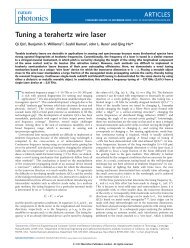
Example of intersection property<br />
C = {x ∈ R n | |p(t)| ≤ 1 for |t| ≤ π/3}<br />
where p(t) = x 1 cost+x 2 cos2t+···+x n cosnt<br />
2<br />
p(t)<br />
1<br />
0<br />
−1<br />
x2<br />
1<br />
0<br />
C<br />
−1<br />
0 π/3 2π/3 π<br />
t<br />
−2<br />
−2 −1 0 1 2<br />
x 1<br />
C is intersection of infinitely many halfspaces, hence convex<br />
<strong>Convex</strong> sets <strong>and</strong> functions 10
<strong>Convex</strong> function<br />
domain domf is a convex set <strong>and</strong> Jensen’s inequality holds:<br />
for all x,y ∈ domf, 0 ≤ θ ≤ 1<br />
f(θx+(1−θ)y) ≤ θf(x)+(1−θ)f(y)<br />
(x,f(x))<br />
(y,f(y))<br />
f is concave if −f is convex<br />
<strong>Convex</strong> sets <strong>and</strong> functions 11
Examples<br />
• linear <strong>and</strong> affine functions are convex <strong>and</strong> concave<br />
• expx, −logx, xlogx are convex<br />
• x α is convex for x > 0 <strong>and</strong> α ≥ 1 or α ≤ 0; |x| α is convex for α ≥ 1<br />
• norms are convex<br />
• quadratic-over-linear function x T x/t is convex in x, t for t > 0<br />
• geometric mean (x 1 x 2···x n ) 1/n is concave for x ≥ 0<br />
• logdetX is concave on set of positive definite matrices<br />
• log(e x 1 +···e x n<br />
) is convex<br />
<strong>Convex</strong> sets <strong>and</strong> functions 12
Epigraph <strong>and</strong> sublevel set<br />
epigraph: epif = {(x,t) | x ∈ domf, f(x) ≤ t}<br />
epif<br />
a function is convex if <strong>and</strong> only its<br />
epigraph is a convex set<br />
f<br />
sublevel sets: C α = {x ∈ domf | f(x) ≤ α}<br />
the sublevel sets of a convex function are convex (converse is false)<br />
<strong>Convex</strong> sets <strong>and</strong> functions 13
Differentiable convex functions<br />
differentiable f is convex if <strong>and</strong> only if domf is convex <strong>and</strong><br />
f(y) ≥ f(x)+∇f(x) T (y −x) for all x,y ∈ domf<br />
f(y)<br />
f(x) + ∇f(x) T (y − x)<br />
(x,f(x))<br />
twice differentiable f is convex if <strong>and</strong> only if domf is convex <strong>and</strong><br />
∇ 2 f(x) ≽ 0 for all x ∈ domf<br />
<strong>Convex</strong> sets <strong>and</strong> functions 14
Establishing convexity of a function<br />
1. verify definition<br />
2. for twice differentiable functions, show ∇ 2 f(x) ≽ 0<br />
3. show that f is obtained from simple convex functions by operations<br />
that preserve convexity<br />
• nonnegative weighted sum<br />
• composition with affine function<br />
• pointwise maximum <strong>and</strong> supremum<br />
• minimization<br />
• composition<br />
• perspective<br />
<strong>Convex</strong> sets <strong>and</strong> functions 15
Positive weighted sum & composition with affine function<br />
nonnegative multiple: αf is convex if f is convex, α ≥ 0<br />
sum: f 1 +f 2 convex if f 1 ,f 2 convex (extends to infinite sums, integrals)<br />
composition with affine function: f(Ax+b) is convex if f is convex<br />
examples<br />
• logarithmic barrier for linear inequalities<br />
f(x) = −<br />
m∑<br />
log(b i −a T i x)<br />
i=1<br />
• (any) norm of affine function: f(x) = ‖Ax+b‖<br />
<strong>Convex</strong> sets <strong>and</strong> functions 16
Pointwise maximum<br />
is convex if f 1 , . . . , f m are convex<br />
f(x) = max{f 1 (x),...,f m (x)}<br />
example: sum of r largest components of x ∈ R n<br />
f(x) = x [1] +x [2] +···+x [r]<br />
is convex (x [i] is ith largest component of x)<br />
proof:<br />
f(x) = max{x i1 +x i2 +···+x ir | 1 ≤ i 1 < i 2 < ··· < i r ≤ n}<br />
<strong>Convex</strong> sets <strong>and</strong> functions 17
Pointwise supremum<br />
g(x) = supf(x,y)<br />
y∈A<br />
is convex if f(x,y) is convex in x for each y ∈ A<br />
examples<br />
• maximum eigenvalue of symmetric matrix<br />
λ max (X) = sup y T Xy<br />
‖y‖ 2 =1<br />
• support function of a set C<br />
S C (x) = supy T x<br />
y∈C<br />
<strong>Convex</strong> sets <strong>and</strong> functions 18
Minimization<br />
h(x) = inf<br />
y∈C f(x,y)<br />
is convex if f(x,y) is convex in (x,y) <strong>and</strong> C is a convex set<br />
examples<br />
• distance to a convex set C: h(x) = inf y∈C ‖x−y‖<br />
• optimal value of linear program as function of righth<strong>and</strong> side<br />
follows by taking<br />
h(x) = inf<br />
y:Ay≤x cT y<br />
f(x,y) = c T y, domf = {(x,y) | Ay ≤ x}<br />
<strong>Convex</strong> sets <strong>and</strong> functions 19
Composition<br />
composition of g : R n → R <strong>and</strong> h : R → R:<br />
f is convex if<br />
f(x) = h(g(x))<br />
g convex, h convex <strong>and</strong> nondecreasing<br />
g concave, h convex <strong>and</strong> nonincreasing<br />
(if we assign h(x) = ∞ for x ∈ domh)<br />
examples<br />
• expg(x) is convex if g is convex<br />
• 1/g(x) is convex if g is concave <strong>and</strong> positive<br />
<strong>Convex</strong> sets <strong>and</strong> functions 20
Vector composition<br />
composition of g : R n → R k <strong>and</strong> h : R k → R:<br />
f is convex if<br />
f(x) = h(g(x)) = h(g 1 (x),g 2 (x),...,g k (x))<br />
g i convex, h convex <strong>and</strong> nondecreasing in each argument<br />
g i concave, h convex <strong>and</strong> nonincreasing in each argument<br />
(if we assign h(x) = ∞ for x ∈ domh)<br />
example<br />
log m ∑<br />
i=1<br />
expg i (x) is convex if g i are convex<br />
<strong>Convex</strong> sets <strong>and</strong> functions 21
Perspective<br />
the perspective of a function f : R n → R is the function g : R n ×R → R,<br />
g(x,t) = tf(x/t)<br />
g is convex if f is convex on domg = {(x,t) | x/t ∈ domf, t > 0}<br />
examples<br />
• perspective of f(x) = x T x is quadratic-over-linear function<br />
g(x,t) = xT x<br />
t<br />
• perspective of negative logarithm f(x) = −logx is relative entropy<br />
g(x,t) = tlogt−tlogx<br />
<strong>Convex</strong> sets <strong>and</strong> functions 22
the conjugate of a function f is<br />
Conjugate function<br />
f ∗ (y) = sup (y T x−f(x))<br />
x∈domf<br />
f(x)<br />
xy<br />
x<br />
(0,−f ∗ (y))<br />
f ∗ is convex (even if f is not)<br />
<strong>Convex</strong> sets <strong>and</strong> functions 23
convex quadratic function (Q ≻ 0)<br />
Examples<br />
f(x) = 1 2 xT Qx<br />
f ∗ (y) = 1 2 yT Q −1 y<br />
negative entropy<br />
norm<br />
f(x) =<br />
n∑<br />
x i logx i f ∗ (y) =<br />
i=1<br />
f(x) = ‖x‖ f ∗ (y) =<br />
n∑<br />
e y i<br />
−1<br />
i=1<br />
{<br />
0 ‖y‖∗ ≤ 1<br />
+∞ otherwise<br />
indicator function (C convex)<br />
f(x) = I C (x) =<br />
{<br />
0 x ∈ C<br />
+∞ otherwise<br />
f ∗ (y) = supy T x<br />
x∈C<br />
<strong>Convex</strong> sets <strong>and</strong> functions 24
<strong>Convex</strong> optimization problems<br />
<strong>Convex</strong> optimization — MLSS 2012<br />
• linear programming<br />
• quadratic programming<br />
• geometric programming<br />
• second-order cone programming<br />
• semidefinite programming
<strong>Convex</strong> optimization problem<br />
minimize f 0 (x)<br />
subject to f i (x) ≤ 0, i = 1,...,m<br />
Ax = b<br />
f 0 , f 1 , . . . , f m are convex functions<br />
• feasible set is convex<br />
• locally optimal points are globally optimal<br />
• tractable, in theory <strong>and</strong> practice<br />
<strong>Convex</strong> optimization problems 25
Linear program (LP)<br />
minimize c T x+d<br />
subject to Gx ≤ h<br />
Ax = b<br />
• inequality is componentwise vector inequality<br />
• convex problem with affine objective <strong>and</strong> constraint functions<br />
• feasible set is a polyhedron<br />
P<br />
x ⋆ −c<br />
<strong>Convex</strong> optimization problems 26
Piecewise-linear minimization<br />
minimize f(x) = max<br />
i=1,...,m (aT i x+b i )<br />
f(x)<br />
a T i x + b i<br />
equivalent linear program<br />
an LP with variables x, t ∈ R<br />
minimize t<br />
subject to a T i x+b i ≤ t, i = 1,...,m<br />
x<br />
<strong>Convex</strong> optimization problems 27
l 1 -Norm <strong>and</strong> l ∞ -norm minimization<br />
l 1 -norm approximation <strong>and</strong> equivalent LP (‖y‖ 1 = ∑ k |y k|)<br />
minimize ‖Ax−b‖ 1<br />
n∑<br />
minimize<br />
i=1<br />
y i<br />
subject to −y ≤ Ax−b ≤ y<br />
l ∞ -norm approximation (‖y‖ ∞ = max k |y k |)<br />
minimize ‖Ax−b‖ ∞<br />
minimize y<br />
subject to −y1 ≤ Ax−b ≤ y1<br />
(1 is vector of ones)<br />
<strong>Convex</strong> optimization problems 28
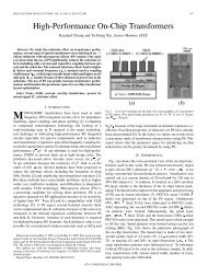
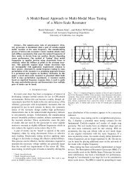
example: histograms of residuals Ax−b (with A is 200×80) for<br />
10<br />
8<br />
6<br />
4<br />
2<br />
01.5<br />
100<br />
80<br />
60<br />
40<br />
20<br />
¡1.5 0<br />
x ls = argmin‖Ax−b‖ 2 , x l1 = argmin‖Ax−b‖ 1<br />
1.0<br />
0.5 0.0 0.5 1.0 1.5<br />
¡¡1.0<br />
(Ax ls −b) k<br />
0.5 0.0 0.5 1.0 1.5<br />
(Ax l1 −b) k<br />
1-norm distribution is wider with a high peak at zero<br />
<strong>Convex</strong> optimization problems 29
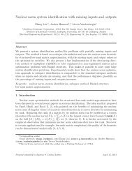
Robust regression<br />
f(t)<br />
25<br />
20<br />
15<br />
10<br />
5<br />
0<br />
¢5<br />
¢10<br />
¢15<br />
¢20<br />
¢10<br />
¢5 0 5 10<br />
t<br />
• 42 points t i , y i (circles), including two outliers<br />
• function f(t) = α+βt fitted using 2-norm (dashed) <strong>and</strong> 1-norm<br />
<strong>Convex</strong> optimization problems 30
Linear discrimination<br />
• given a set of points {x 1 ,...,x N } with binary labels s i ∈ {−1,1}<br />
• find hyperplane a T x+b = 0 that strictly separates the two classes<br />
a T x i +b > 0 if s i = 1<br />
a T x i +b < 0 if s i = −1<br />
homogeneous in a, b, hence equivalent to the linear inequalities (in a, b)<br />
s i (a T x i +b) ≥ 1, i = 1,...,N<br />
<strong>Convex</strong> optimization problems 31
Approximate linear separation of non-separable sets<br />
minimize<br />
N∑<br />
max{0,1−s i (a T x i +b)}<br />
i=1<br />
• a piecewise-linear minimization problem in a, b; equivalent to an LP<br />
• can be interpreted as a heuristic for minimizing #misclassified points<br />
<strong>Convex</strong> optimization problems 32
Quadratic program (QP)<br />
minimize (1/2)x T Px+q T x+r<br />
subject to Gx ≤ h<br />
• P ∈ S n +, so objective is convex quadratic<br />
• minimize a convex quadratic function over a polyhedron<br />
P<br />
x ⋆ −∇f 0 (x ⋆ )<br />
<strong>Convex</strong> optimization problems 33
Linear program with r<strong>and</strong>om cost<br />
minimize c T x<br />
subject to Gx ≤ h<br />
• c is r<strong>and</strong>om vector with mean ¯c <strong>and</strong> covariance Σ<br />
• hence, c T x is r<strong>and</strong>om variable with mean ¯c T x <strong>and</strong> variance x T Σx<br />
expected cost-variance trade-off<br />
minimize Ec T x+γvar(c T x) = ¯c T x+γx T Σx<br />
subject to Gx ≤ h<br />
γ > 0 is risk aversion parameter<br />
<strong>Convex</strong> optimization problems 34
Robust linear discrimination<br />
H 1 = {z | a T z +b = 1}<br />
H −1 = {z | a T z +b = −1}<br />
distance between hyperplanes is 2/‖a‖ 2<br />
to separate two sets of points by maximum margin,<br />
minimize ‖a‖ 2 2 = a T a<br />
subject to s i (a T x i +b) ≥ 1, i = 1,...,N<br />
a quadratic program in a, b<br />
<strong>Convex</strong> optimization problems 35
Support vector classifier<br />
minimize γ‖a‖ 2 2+<br />
N∑<br />
max{0,1−s i (a T x i +b)}<br />
i=1<br />
γ = 0 γ = 10<br />
equivalent to a quadratic program<br />
<strong>Convex</strong> optimization problems 36
Kernel formulation<br />
minimize f(Xa)+‖a‖ 2 2<br />
• variables a ∈ R n<br />
• X ∈ R N×n with N ≤ n <strong>and</strong> rank N<br />
change of variables<br />
y = Xa,<br />
a = X T (XX T ) −1 y<br />
• a is minimum-norm solution of Xa = y<br />
• gives convex problem with N variables y<br />
minimize f(y)+y T Q −1 y<br />
Q = XX T is kernel matrix<br />
<strong>Convex</strong> optimization problems 37
Total variation signal reconstruction<br />
minimize ‖ˆx−x cor ‖ 2 2+γφ(ˆx)<br />
• x cor = x+v is corrupted version of unknown signal x, with noise v<br />
• variable ˆx (reconstructed signal) is estimate of x<br />
• φ : R n → R is quadratic or total variation smoothing penalty<br />
φ quad (ˆx) =<br />
n−1<br />
∑<br />
(ˆx i+1 − ˆx i ) 2 , φ tv (ˆx) =<br />
i=1<br />
n−1<br />
∑<br />
i=1<br />
|ˆx i+1 − ˆx i |<br />
<strong>Convex</strong> optimization problems 38
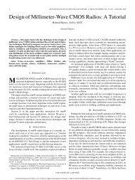
example: x cor , <strong>and</strong> reconstruction with quadratic <strong>and</strong> t.v. smoothing<br />
2<br />
xcor<br />
0<br />
£2<br />
2<br />
0 500 1000 1500 2000<br />
i<br />
quad.<br />
0<br />
£2<br />
2<br />
0 500 1000 1500 2000<br />
i<br />
t.v.<br />
0<br />
£2<br />
0 500 1000 1500 2000<br />
i<br />
• quadratic smoothing smooths out noise <strong>and</strong> sharp transitions in signal<br />
• total variation smoothing preserves sharp transitions in signal<br />
<strong>Convex</strong> optimization problems 39
Geometric programming<br />
posynomial function<br />
f(x) =<br />
K∑<br />
k=1<br />
c k x a 1k<br />
1 xa 2k<br />
2 ···x a nk<br />
n , domf = R n ++<br />
with c k > 0<br />
geometric program (GP)<br />
with f i posynomial<br />
minimize f 0 (x)<br />
subject to f i (x) ≤ 1, i = 1,...,m<br />
<strong>Convex</strong> optimization problems 40
Geometric program in convex form<br />
change variables to<br />
y i = logx i ,<br />
<strong>and</strong> take logarithm of cost, constraints<br />
geometric program in convex form:<br />
( K<br />
∑<br />
)<br />
minimize log exp(a T 0ky +b 0k )<br />
( k=1<br />
∑ K<br />
)<br />
subject to log<br />
exp(a T iky +b ik )<br />
≤ 0, i = 1,...,m<br />
k=1<br />
b ik = logc ik<br />
<strong>Convex</strong> optimization problems 41
Second-order cone program (SOCP)<br />
minimize f T x<br />
subject to ‖A i x+b i ‖ 2 ≤ c T i x+d i, i = 1,...,m<br />
• ‖·‖ 2 is Euclidean norm ‖y‖ 2 = √ y 2 1 +···+y2 n<br />
• constraints are nonlinear, nondifferentiable, convex<br />
1<br />
constraints are inequalities<br />
w.r.t. second-order cone:<br />
{<br />
y<br />
√ }<br />
∣ y1 2+···+y2 p−1 ≤ y p<br />
y3<br />
0.5<br />
0<br />
1<br />
0<br />
0<br />
1<br />
y 2<br />
−1<br />
−1<br />
y 1<br />
<strong>Convex</strong> optimization problems 42
Robust linear program (stochastic)<br />
minimize c T x<br />
subject to prob(a T i x ≤ b i) ≥ η, i = 1,...,m<br />
• a i r<strong>and</strong>om <strong>and</strong> normally distributed with mean ā i , covariance Σ i<br />
• we require that x satisfies each constraint with probability exceeding η<br />
η = 10% η = 50% η = 90%<br />
<strong>Convex</strong> optimization problems 43
SOCP formulation<br />
the ‘chance constraint’ prob(a T i x ≤ b i) ≥ η is equivalent to the constraint<br />
ā T i x+Φ −1 (η)‖Σ 1/2<br />
i x‖ 2 ≤ b i<br />
Φ is the (unit) normal cumulative density function<br />
1<br />
η<br />
Φ(t)<br />
0.5<br />
0<br />
0<br />
t<br />
Φ −1 (η)<br />
robust LP is a second-order cone program for η ≥ 0.5<br />
<strong>Convex</strong> optimization problems 44
Robust linear program (deterministic)<br />
minimize c T x<br />
subject to a T i x ≤ b i for all a i ∈ E i , i = 1,...,m<br />
• a i uncertain but bounded by ellipsoid E i = {ā i +P i u | ‖u‖ 2 ≤ 1}<br />
• we require that x satisfies each constraint for all possible a i<br />
SOCP formulation<br />
minimize c T x<br />
subject to ā T i x+‖PT i x‖ 2 ≤ b i , i = 1,...,m<br />
follows from<br />
sup (ā i +P i u) T x = ā T i x+‖Pi T x‖ 2<br />
‖u‖ 2 ≤1<br />
<strong>Convex</strong> optimization problems 45
Examples of second-order cone constraints<br />
convex quadratic constraint (A = LL T positive definite)<br />
x T Ax+2b T x+c ≤ 0<br />
⇕<br />
∥ L T x+L −1 b ∥ 2<br />
≤ (b T A −1 b−c) 1/2<br />
extends to positive semidefinite singular A<br />
hyperbolic constraint<br />
[<br />
∥<br />
x T x ≤ yz, y,z ≥ 0<br />
2x<br />
y −z<br />
⇕<br />
]∥ ∥∥∥2<br />
≤ y +z, y,z ≥ 0<br />
<strong>Convex</strong> optimization problems 46
Examples of SOC-representable constraints<br />
positive powers<br />
x 1.5 ≤ t, x ≥ 0<br />
⇕<br />
∃z : x 2 ≤ tz, z 2 ≤ x, x,z ≥ 0<br />
• two hyperbolic constraints can be converted to SOC constraints<br />
• extends to powers x p for rational p ≥ 1<br />
negative powers<br />
x −3 ≤ t, x > 0<br />
⇕<br />
∃z : 1 ≤ tz, z 2 ≤ tx, x,z ≥ 0<br />
• two hyperbolic constraints on r.h.s. can be converted to SOC constraints<br />
• extends to powers x p for rational p < 0<br />
<strong>Convex</strong> optimization problems 47
Semidefinite program (SDP)<br />
minimize c T x<br />
subject to x 1 A 1 +x 2 A 2 +···+x n A n ≼ B<br />
• A 1 , A 2 , . . . , A n , B are symmetric matrices<br />
• inequality X ≼ Y means Y −X is positive semidefinite, i.e.,<br />
z T (Y −X)z = ∑ i,j<br />
(Y ij −X ij )z i z j ≥ 0 for all z<br />
• includes many nonlinear constraints as special cases<br />
<strong>Convex</strong> optimization problems 48
Geometry<br />
1<br />
[<br />
x y<br />
y z<br />
]<br />
≽ 0<br />
z<br />
0.5<br />
1 0<br />
0<br />
y<br />
−1<br />
0<br />
0.5<br />
x<br />
1<br />
• a nonpolyhedral convex cone<br />
• feasible set of a semidefinite program is the intersection of the positive<br />
semidefinite cone in high dimension with planes<br />
<strong>Convex</strong> optimization problems 49
Examples<br />
A(x) = A 0 +x 1 A 1 +···+x m A m (A i ∈ S n )<br />
eigenvalue minimization (<strong>and</strong> equivalent SDP)<br />
minimize λ max (A(x))<br />
minimize t<br />
subject to A(x) ≼ tI<br />
matrix-fractional function<br />
minimize b T A(x) −1 b<br />
subject to A(x) ≽ 0<br />
minimize t[ A(x) b<br />
subject to<br />
b T t<br />
]<br />
≽ 0<br />
<strong>Convex</strong> optimization problems 50
Matrix norm minimization<br />
A(x) = A 0 +x 1 A 1 +x 2 A 2 +···+x n A n (A i ∈ R p×q )<br />
matrix norm approximation (‖X‖ 2 = max k σ k (X))<br />
minimize ‖A(x)‖ 2<br />
minimize t[<br />
subject to<br />
tI<br />
A(x)<br />
A(x) T<br />
tI<br />
]<br />
≽ 0<br />
nuclear norm approximation (‖X‖ ∗ = ∑ k σ k(X))<br />
minimize ‖A(x)‖ ∗<br />
minimize (trU +trV)/2<br />
[<br />
U A(x)<br />
subject to<br />
T<br />
A(x) V<br />
]<br />
≽ 0<br />
<strong>Convex</strong> optimization problems 51
Semidefinite relaxation<br />
semidefinite programming is often used<br />
• to find good bounds for nonconvex polynomial problems, via relaxation<br />
• as a heuristic for good suboptimal points<br />
example: Boolean least-squares<br />
minimize ‖Ax−b‖ 2 2<br />
subject to x 2 i = 1, i = 1,...,n<br />
• basic problem in digital communications<br />
• could check all 2 n possible values of x ∈ {−1,1} n . . .<br />
• an NP-hard problem, <strong>and</strong> very hard in general<br />
<strong>Convex</strong> optimization problems 52
Lifting<br />
Boolean least-squares problem<br />
minimize x T A T Ax−2b T Ax+b T b<br />
subject to x 2 i = 1, i = 1,...,n<br />
reformulation: introduce new variable Y = xx T<br />
minimize tr(A T AY)−2b T Ax+b T b<br />
subject to Y = xx T<br />
diag(Y) = 1<br />
• cost function <strong>and</strong> second constraint are linear (in the variables Y, x)<br />
• first constraint is nonlinear <strong>and</strong> nonconvex<br />
. . . still a very hard problem<br />
<strong>Convex</strong> optimization problems 53
Relaxation<br />
replace Y = xx T with weaker constraint Y ≽ xx T to obtain relaxation<br />
minimize tr(A T AY)−2b T Ax+b T b<br />
subject to Y ≽ xx T<br />
diag(Y) = 1<br />
• convex; can be solved as a semidefinite program<br />
Y ≽ xx T<br />
⇐⇒<br />
[ Y x<br />
x T 1<br />
]<br />
≽ 0<br />
• optimal value gives lower bound for Boolean LS problem<br />
• if Y = xx T at the optimum, we have solved the exact problem<br />
• otherwise, can use r<strong>and</strong>omized rounding<br />
generate z from N(x,Y −xx T ) <strong>and</strong> take x = sign(z)<br />
<strong>Convex</strong> optimization problems 54
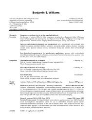
Example<br />
0.5<br />
0.4<br />
SDP bound<br />
LS solution<br />
frequency<br />
0.3<br />
0.2<br />
0.1<br />
0<br />
1 1.2<br />
‖Ax − b‖ 2 /(SDP bound)<br />
• n = 100: feasible set has 2 100 ≈ 10 30 points<br />
• histogram of 1000 r<strong>and</strong>omized solutions from SDP relaxation<br />
<strong>Convex</strong> optimization problems 55
Overview<br />
1. Basic theory <strong>and</strong> convex modeling<br />
• convex sets <strong>and</strong> functions<br />
• common problem classes <strong>and</strong> applications<br />
2. Interior-point methods for conic optimization<br />
• conic optimization<br />
• barrier methods<br />
• symmetric primal-dual methods<br />
3. First-order methods<br />
• (proximal) gradient algorithms<br />
• dual techniques <strong>and</strong> multiplier methods
Conic optimization<br />
<strong>Convex</strong> optimization — MLSS 2012<br />
• definitions <strong>and</strong> examples<br />
• modeling<br />
• duality
Generalized (conic) inequalities<br />
conic inequality: a constraint x ∈ K with K a convex cone in R m<br />
we require that K is a proper cone:<br />
• closed<br />
• pointed: does not contain a line (equivalently, K ∩(−K) = {0}<br />
• with nonempty interior: intK ≠ ∅ (equivalently, K +(−K) = R m )<br />
notation<br />
x ≽ K y ⇐⇒ x−y ∈ K,<br />
x ≻ K y ⇐⇒ x−y ∈ intK<br />
subscript in ≽ K is omitted if K is clear from the context<br />
Conic optimization 56
Cone linear program<br />
minimize c T x<br />
subject to Ax ≼ K b<br />
if K is the nonnegative orthant, this is a (regular) linear program<br />
widely used in recent literature on convex optimization<br />
• modeling: a small number of ‘primitive’ cones is sufficient to express<br />
most convex constraints that arise in practice<br />
• algorithms: a convenient problem format when extending interior-point<br />
algorithms for linear programming to convex optimization<br />
Conic optimization 57
Norm cone<br />
K = { (x,y) ∈ R m−1 ×R | ‖x‖ ≤ y }<br />
1<br />
y<br />
0.5<br />
1 0<br />
0<br />
x 2<br />
−1<br />
−1<br />
x 1<br />
0<br />
1<br />
for the Euclidean norm this is the second-order cone (notation: Q m )<br />
Conic optimization 58
Second-order cone program<br />
minimize c T x<br />
subject to ‖B k0 x+d k0 ‖ 2<br />
≤ B k1 x+d k1 , k = 1,...,r<br />
cone LP formulation: express constraints as Ax ≼ K b<br />
K = Q m 1<br />
×···×Q m r<br />
, A =<br />
⎡<br />
⎢<br />
⎣<br />
⎤<br />
−B 10<br />
−B 11<br />
.<br />
−B<br />
⎥<br />
r0 ⎦<br />
−B r1<br />
, b =<br />
⎡<br />
⎢<br />
⎣<br />
⎤<br />
d 10<br />
d 11<br />
.<br />
d<br />
⎥<br />
r0 ⎦<br />
d r1<br />
(assuming B k0 , d k0 have m k −1 rows)<br />
Conic optimization 59
Vector notation for symmetric matrices<br />
• vectorized symmetric matrix: for U ∈ S p<br />
vec(U) = √ 2<br />
(<br />
U11<br />
√ , U 21 , ..., U p1 , U 22<br />
√ , U 32 , ..., U p2 , ..., U )<br />
pp<br />
√<br />
2 2 2<br />
• inverse operation: for u = (u 1 ,u 2 ,...,u n ) ∈ R n with n = p(p+1)/2<br />
⎡<br />
mat(u) = √ 1 ⎢<br />
2<br />
⎣<br />
√ ⎤<br />
2u1<br />
√<br />
u 2 ··· u p<br />
u 2 2up+1 ··· u 2p−1<br />
⎥<br />
. . . ⎦<br />
√<br />
u p u 2p−1 ··· 2up(p+1)/2<br />
coefficients √ 2 are added so that st<strong>and</strong>ard inner products are preserved:<br />
tr(UV) = vec(U) T vec(V),<br />
u T v = tr(mat(u)mat(v))<br />
Conic optimization 60
Positive semidefinite cone<br />
S p = {vec(X) | X ∈ S p +} = {x ∈ R p(p+1)/2 | mat(x) ≽ 0}<br />
1<br />
z<br />
0.5<br />
0<br />
1<br />
0<br />
y<br />
−1<br />
0<br />
x<br />
0.5<br />
1<br />
S 2 =<br />
{<br />
(x,y,z)<br />
∣<br />
[<br />
x y/ √ 2<br />
y/ √ 2 z<br />
]<br />
}<br />
≽ 0<br />
Conic optimization 61
Semidefinite program<br />
minimize c T x<br />
subject to x 1 A 11 +x 2 A 12 +···+x n A 1n ≼ B 1<br />
...<br />
x 1 A r1 +x 2 A r2 +···+x n A rn ≼ B r<br />
r linear matrix inequalities of order p 1 , . . . , p r<br />
cone LP formulation: express constraints as Ax ≼ K B<br />
K = S p 1 ×S p 2 ×···×S p r<br />
A =<br />
⎡<br />
⎢<br />
⎣<br />
vec(A 11 ) vec(A 12 ) ··· vec(A 1n )<br />
vec(A 21 ) vec(A 22 ) ··· vec(A 2n )<br />
. . .<br />
vec(A r1 ) vec(A r2 ) ··· vec(A rn )<br />
⎤<br />
⎥<br />
⎦ ,<br />
⎡<br />
b = ⎢<br />
⎣<br />
vec(B 1 )<br />
vec(B 2 )<br />
.<br />
vec(B r )<br />
⎤<br />
⎥<br />
⎦<br />
Conic optimization 62
Exponential cone<br />
the epigraph of the perspective of expx is a non-proper cone<br />
{<br />
}<br />
K = (x,y,z) ∈ R 3 | ye x/y ≤ z, y > 0<br />
the exponential cone is K exp = clK = K ∪{(x,0,z) | x ≤ 0,z ≥ 0}<br />
1<br />
z<br />
0.5<br />
0<br />
3<br />
2<br />
y<br />
1<br />
0<br />
−2<br />
−1<br />
x<br />
0<br />
1<br />
Conic optimization 63
Geometric program<br />
minimize c T x<br />
subject to log<br />
∑n i<br />
k=1<br />
exp(a T ik x+b ik) ≤ 0, i = 1,...,r<br />
cone LP formulation<br />
minimize c T x<br />
⎡<br />
subject to<br />
⎣ aT ik x+b ik<br />
1<br />
z ik<br />
∑n i<br />
k=1<br />
⎤<br />
⎦ ∈ K exp , k = 1,...,n i , i = 1,...,r<br />
z ik ≤ 1, i = 1,...,m<br />
Conic optimization 64
Power cone<br />
definition: for α = (α 1 ,α 2 ,...,α m ) > 0,<br />
m∑<br />
i=1<br />
α i = 1<br />
K α = { (x,y) ∈ R m + ×R | |y| ≤ x α }<br />
1<br />
1 ···xα m<br />
m<br />
examples for m = 2<br />
α = ( 1 2 , 1 2 ) α = (2 3 , 1 3 ) α = (3 4 , 1 4 )<br />
0.5<br />
0.5<br />
0.4<br />
0.2<br />
y<br />
0<br />
y<br />
0<br />
y<br />
0<br />
−0.2<br />
−0.4<br />
0<br />
0.5<br />
1 0<br />
0.5<br />
x 1 x 2<br />
1<br />
−0.5<br />
0<br />
0.5<br />
1 0<br />
0.5<br />
x 1<br />
x 2<br />
1<br />
−0.5<br />
0<br />
0.5<br />
1 0 0.5 1<br />
x 1<br />
x 2<br />
Conic optimization 65
Outline<br />
• definition <strong>and</strong> examples<br />
• modeling<br />
• duality
<strong>Modeling</strong> software<br />
modeling packages for convex optimization<br />
• CVX, YALMIP (MATLAB)<br />
• CVXPY, CVXMOD (Python)<br />
assist the user in formulating convex problems, by automating two tasks:<br />
• verifying convexity from convex calculus rules<br />
• transforming problem in input format required by st<strong>and</strong>ard solvers<br />
related packages<br />
general-purpose optimization modeling: AMPL, GAMS<br />
Conic optimization 66
CVX example<br />
minimize ‖Ax−b‖ 1<br />
subject to 0 ≤ x k ≤ 1, k = 1,...,n<br />
MATLAB code<br />
cvx_begin<br />
variable x(3);<br />
minimize(norm(A*x - b, 1))<br />
subject to<br />
x >= 0;<br />
x
<strong>Modeling</strong> <strong>and</strong> conic optimization<br />
convex modeling systems (CVX, YALMIP, CVXPY, CVXMOD, . . . )<br />
• convert problems stated in st<strong>and</strong>ard mathematical notation to cone LPs<br />
• in principle, any convex problem can be represented as a cone LP<br />
• in practice, a small set of primitive cones is used (R n +, Q p , S p )<br />
• choice of cones is limited by available algorithms <strong>and</strong> solvers (see later)<br />
modeling systems implement set of rules for expressing constraints<br />
f(x) ≤ t<br />
as conic inequalities for the implemented cones<br />
Conic optimization 68
Examples of second-order cone representable functions<br />
• convex quadratic<br />
f(x) = x T Px+q T x+r (P ≽ 0)<br />
• quadratic-over-linear function<br />
f(x,y) = xT x<br />
y<br />
with domf = R n ×R + (assume 0/0 = 0)<br />
• convex powers with rational exponent<br />
f(x) = |x| α , f(x) =<br />
{<br />
x<br />
β<br />
x > 0<br />
+∞ x ≤ 0<br />
for rational α ≥ 1 <strong>and</strong> β ≤ 0<br />
• p-norm f(x) = ‖x‖ p for rational p ≥ 1<br />
Conic optimization 69
Examples of SD cone representable functions<br />
• matrix-fractional function<br />
f(X,y) = y T X −1 y with domf = {(X,y) ∈ S n +×R n | y ∈ R(X)}<br />
• maximum eigenvalue of symmetric matrix<br />
• maximum singular value f(X) = ‖X‖ 2 = σ 1 (X)<br />
[ ] tI X<br />
‖X‖ 2 ≤ t ⇐⇒<br />
X T tI<br />
≽ 0<br />
• nuclear norm f(X) = ‖X‖ ∗ = ∑ i σ i(X)<br />
‖X‖ ∗ ≤ t ⇐⇒ ∃U,V :<br />
[ U X<br />
X T V<br />
]<br />
≽ 0,<br />
1<br />
(trU +trV) ≤ t<br />
2<br />
Conic optimization 70
Functions representable with exponential <strong>and</strong> power cone<br />
exponential cone<br />
• exponential <strong>and</strong> logarithm<br />
• entropy f(x) = xlogx<br />
power cone<br />
• increasing power of absolute value: f(x) = |x| p with p ≥ 1<br />
• decreasing power: f(x) = x q with q ≤ 0 <strong>and</strong> domain R ++<br />
• p-norm: f(x) = ‖x‖ p with p ≥ 1<br />
Conic optimization 71
Outline<br />
• definition <strong>and</strong> examples<br />
• modeling<br />
• duality
Linear programming duality<br />
primal <strong>and</strong> dual LP<br />
(P) minimize c T x<br />
subject to Ax ≤ b<br />
(D) maximize −b T z<br />
subject to A T z +c = 0<br />
z ≥ 0<br />
• primal optimal value is p ⋆ (+∞ if infeasible, −∞ if unbounded below)<br />
• dual optimal value is d ⋆ (−∞ if infeasible, +∞ if unbounded below)<br />
duality theorem<br />
• weak duality: p ⋆ ≥ d ⋆ , with no exception<br />
• strong duality: p ⋆ = d ⋆ if primal or dual is feasible<br />
• if p ⋆ = d ⋆ is finite, then primal <strong>and</strong> dual optima are attained<br />
Conic optimization 72
Dual cone<br />
definition<br />
K ∗ = {y | x T y ≥ 0 for all x ∈ K}<br />
K ∗ is a proper cone if K is a proper cone<br />
dual inequality: x ≽ ∗ y means x ≽ K ∗ y for generic proper cone K<br />
note: dual cone depends on choice of inner product:<br />
H −1 K ∗<br />
is dual cone for inner product 〈x,y〉 = x T Hy<br />
Conic optimization 73
Examples<br />
• R p +, Q p , S p are self-dual: K = K ∗<br />
• dual of a norm cone is the norm cone of the dual norm<br />
• dual of exponential cone<br />
K ∗ exp = { (u,v,w) ∈ R − ×R×R + | −ulog(−u/w)+u−v ≤ 0 }<br />
(with 0log(0/w) = 0 if w ≥ 0)<br />
• dual of power cone is<br />
K ∗ α = { (u,v) ∈ R m + ×R | |v| ≤ (u 1 /α 1 ) α1···(u m /α m ) α m }<br />
Conic optimization 74
Primal <strong>and</strong> dual cone LP<br />
primal problem (optimal value p ⋆ )<br />
minimize c T x<br />
subject to Ax ≼ b<br />
dual problem (optimal value d ⋆ )<br />
maximize −b T z<br />
subject to A T z +c = 0<br />
z ≽ ∗ 0<br />
weak duality: p ⋆ ≥ d ⋆ (without exception)<br />
Conic optimization 75
Strong duality<br />
p ⋆ = d ⋆<br />
if primal or dual is strictly feasible<br />
• slightly weaker than LP duality (which only requires feasibility)<br />
• can have d ⋆ < p ⋆ with finite p ⋆ <strong>and</strong> d ⋆<br />
other implications of strict feasibility<br />
• if primal is strictly feasible, then dual optimum is attained (if d ⋆ is finite)<br />
• if dual is strictly feasible, then primal optimum is attained (if p ⋆ is finite)<br />
Conic optimization 76
Optimality conditions<br />
minimize c T x<br />
subject to Ax+s = b<br />
s ≽ 0<br />
maximize −b T z<br />
subject to A T z +c = 0<br />
z ≽ ∗ 0<br />
optimality conditions<br />
[<br />
0<br />
s<br />
]<br />
=<br />
[<br />
0 A<br />
T<br />
−A 0<br />
][<br />
x<br />
z<br />
]<br />
+<br />
[<br />
c<br />
b<br />
]<br />
s ≽ 0, z ≽ ∗ 0, z T s = 0<br />
duality gap: inner product of (x,z) <strong>and</strong> (0,s) gives<br />
z T s = c T x+b T z<br />
Conic optimization 77
Barrier methods<br />
<strong>Convex</strong> optimization — MLSS 2012<br />
• barrier method for linear programming<br />
• normal barriers<br />
• barrier method for conic optimization
History<br />
• 1960s: Sequentially Unconstrained Minimization Technique (SUMT)<br />
solves nonlinear convex optimization problem<br />
minimize f 0 (x)<br />
subject to f i (x) ≤ 0, i = 1,...,m<br />
via a sequence of unconstrained minimization problems<br />
minimize tf 0 (x)− m ∑<br />
i=1<br />
log(−f i (x))<br />
• 1980s: LP barrier methods with polynomial worst-case complexity<br />
• 1990s: barrier methods for non-polyhedral cone LPs<br />
Barrier methods 78
Logarithmic barrier function for linear inequalities<br />
• barrier for nonnegative orthant R m +: φ(s) = − m ∑<br />
• barrier for inequalities Ax ≤ b:<br />
i=1<br />
logs i<br />
ψ(x) = φ(b−Ax) = −<br />
m∑<br />
log(b i −a T i x)<br />
i=1<br />
convex, ψ(x) → ∞ at boundary of domψ = {x | Ax < b}<br />
gradient <strong>and</strong> Hessian<br />
∇ψ(x) = −A T ∇φ(s),<br />
∇ 2 ψ(x) = A T ∇φ 2 (s)A<br />
with s = b−Ax <strong>and</strong><br />
∇φ(s) = −( 1<br />
s 1<br />
,...,<br />
) (<br />
1<br />
1<br />
, ∇φ 2 (s) = diag<br />
s m s 2 ,...,<br />
1<br />
1<br />
s 2 m<br />
)<br />
Barrier methods 79
Central path for linear program<br />
minimize c T x<br />
subject to Ax ≤ b<br />
central path: minimizers x ⋆ (t) of<br />
c<br />
f t (x) = tc T x+φ(b−Ax)<br />
t is a positive parameter<br />
x ⋆<br />
x ⋆ (t)<br />
optimality conditions: x = x ⋆ (t) satisfies<br />
∇f t (x) = tc−A T ∇φ(s) = 0,<br />
s = b−Ax<br />
Barrier methods 80
Central path <strong>and</strong> duality<br />
dual feasible point on central path<br />
• for x = x ⋆ (t) <strong>and</strong> s = b−Ax,<br />
z ∗ (t) = − 1 t ∇φ(s) = ( 1<br />
ts 1<br />
,<br />
1<br />
ts 2<br />
,...,<br />
)<br />
1<br />
ts m<br />
z = z ⋆ (t) is strictly dual feasible: c+A T z = 0 <strong>and</strong> z > 0<br />
• can be corrected to account for inexact centering of x ≈ x ⋆ (t)<br />
duality gap between x = x ⋆ (t) <strong>and</strong> z = z ⋆ (t) is<br />
c T x+b T z = s T z = m t<br />
gives bound on suboptimality: c T x ⋆ (t)−p ⋆ ≤ m/t<br />
Barrier methods 81
Barrier method<br />
starting with t > 0, strictly feasible x<br />
• make one or more Newton steps to (approximately) minimize f t :<br />
x + = x−α∇ 2 f t (x) −1 ∇f t (x)<br />
step size α is fixed or from line search<br />
• increase t <strong>and</strong> repeat until c T x−p ⋆ ≤ ǫ<br />
complexity: with proper initialization, step size, update scheme for t,<br />
#Newton steps = O (√ mlog(1/ǫ) )<br />
result follows from convergence analysis of Newton’s method for f t<br />
Barrier methods 82
Outline<br />
• barrier method for linear programming<br />
• normal barriers<br />
• barrier method for conic optimization
Normal barrier for proper cone<br />
φ is a θ-normal barrier for the proper cone K if it is<br />
• a barrier: smooth, convex, domain intK, blows up at boundary of K<br />
• logarithmically homogeneous with parameter θ:<br />
φ(tx) = φ(x)−θlogt, ∀x ∈ intK, t > 0<br />
• self-concordant: restriction g(α) = φ(x+αv) to any line satisfies<br />
g ′′′ (α) ≤ 2g ′′ (α) 3/2<br />
(Nesterov <strong>and</strong> Nemirovski, 1994)<br />
Barrier methods 83
Examples<br />
nonnegative orthant: K = R m +<br />
φ(x) = −<br />
m∑<br />
logx i (θ = m)<br />
i=1<br />
second-order cone: K = Q p = {(x,y) ∈ R p−1 ×R | ‖x‖ 2 ≤ y}<br />
φ(x,y) = −log(y 2 −x T x) (θ = 2)<br />
semidefinite cone: K = S m = {x ∈ R m(m+1)/2 | mat(x) ≽ 0}<br />
φ(x) = −logdetmat(x) (θ = m)<br />
Barrier methods 84
exponential cone: K exp = cl{(x,y,z) ∈ R 3 | ye x/y ≤ z, y > 0}<br />
φ(x,y,z) = −log(ylog(z/y)−x)−logz −logy (θ = 3)<br />
power cone: K = {(x 1 ,x 2 ,y) ∈ R + ×R + ×R | |y| ≤ x α 1<br />
1 xα 2<br />
2 }<br />
φ(x,y) = −log<br />
(<br />
x 2α 1<br />
1 x 2α 2<br />
2 −y 2) −logx 1 −logx 2 (θ = 4)<br />
Barrier methods 85
Central path<br />
conic LP (with inequality with respect to proper cone K)<br />
minimize c T x<br />
subject to Ax ≼ b<br />
barrier for the feasible set<br />
where φ is a θ-normal barrier for K<br />
φ(b−Ax)<br />
central path: set of minimizers x ⋆ (t) (with t > 0) of<br />
f t (x) = tc T x+φ(b−Ax)<br />
Barrier methods 86
Newton step<br />
centering problem<br />
minimize f t (x) = tc T x+φ(b−Ax)<br />
Newton step at x<br />
∆x = −∇ 2 f t (x) −1 ∇f t (x)<br />
Newton decrement<br />
λ t (x) = ( ∆x T ∇ 2 f t (x)∆x ) 1/2<br />
= ( −∇f t (x) T ∆x ) 1/2<br />
useful as a measure of proximity of x to x ⋆ (t)<br />
Barrier methods 87
Damped Newton method<br />
minimize f t (x) = tc T x+φ(b−Ax)<br />
algorithm (with parameters ǫ ∈ (0,1/2), η ∈ (0,1/4])<br />
select a starting point x ∈ domf t<br />
repeat:<br />
1. compute Newton step ∆x <strong>and</strong> Newton decrement λ t (x)<br />
2. if λ t (x) 2 ≤ ǫ, return x<br />
3. otherwise, set x := x+α∆x with<br />
α =<br />
1<br />
1+λ t (x)<br />
if λ t (x) ≥ η,<br />
α = 1 if λ t (x) < η<br />
• stopping criterion λ t (x) 2 ≤ ǫ implies f t (x)−inff t (x) ≤ ǫ<br />
• alternatively, can use backtracking line search<br />
Barrier methods 88
Convergence results for damped Newton method<br />
• damped Newton phase: f t decreases by at least a positive constant γ<br />
f t (x + )−f t (x) ≤ −γ if λ t (x) ≥ η<br />
where γ = η −log(1+η)<br />
• quadratic convergence phase: λ t rapidly decreases to zero<br />
2λ t (x + ) ≤ (2λ t (x)) 2<br />
if λ t (x) < η<br />
implies λ t (x + ) ≤ 2η 2 < η<br />
conclusion: the number of Newton iterations is bounded by<br />
f t (x (0) )−inff t (x)<br />
γ<br />
+log 2 log 2 (1/ǫ)<br />
Barrier methods 89
Outline<br />
• barrier method for linear programming<br />
• normal barriers<br />
• barrier method for conic optimization
Central path <strong>and</strong> duality<br />
x ⋆ (t) = argmin ( tc T x+φ(b−Ax) )<br />
duality point on central path: x ⋆ (t) defines a strictly dual feasible z ⋆ (t)<br />
z ⋆ (t) = − 1 t ∇φ(s),<br />
s = b−Ax⋆ (t)<br />
duality gap: gap between x = x ⋆ (t) <strong>and</strong> z = z ⋆ (t) is<br />
c T x+b T z = s T z = θ t ,<br />
cT x−p ⋆ ≤ θ t<br />
extension near central path (for λ t (x) < 1): c T x−p ⋆ ≤<br />
(<br />
1+ λ t(x)<br />
√<br />
θ<br />
) θ<br />
t<br />
(results follow from properties of normal barriers)<br />
Barrier methods 90
Short-step barrier method<br />
algorithm (parameters ǫ ∈ (0,1), β = 1/8)<br />
• select initial x <strong>and</strong> t with λ t (x) ≤ β<br />
• repeat until 2θ/t ≤ ǫ:<br />
( )<br />
1<br />
t := 1+<br />
1+8 √ t, x := x−∇f t (x) −1 ∇f t (x)<br />
θ<br />
properties<br />
• increases t slowly so x stays in region of quadratic region (λ t (x) ≤ β)<br />
• iteration complexity<br />
#iterations = O<br />
( √θlog<br />
( θ<br />
ǫt 0<br />
))<br />
• best known worst-case complexity; same as for linear programming<br />
Barrier methods 91
Predictor-corrector methods<br />
short-step barrier methods<br />
• stay in narrow neighborhood of central path (defined by limit on λ t )<br />
• make small, fixed increases t + = µt<br />
as a result, quite slow in practice<br />
predictor-corrector method<br />
• select new t using a linear approximation to central path (‘predictor’)<br />
• re-center with new t (‘corrector’)<br />
allows faster <strong>and</strong> ‘adaptive’ increases in t; similar worst-case complexity<br />
Barrier methods 92
Primal-dual methods<br />
<strong>Convex</strong> optimization — MLSS 2012<br />
• primal-dual algorithms for linear programming<br />
• symmetric cones<br />
• primal-dual algorithms for conic optimization<br />
• implementation
Primal-dual interior-point methods<br />
similarities with barrier method<br />
• follow the same central path<br />
• same linear algebra cost per iteration<br />
differences<br />
• more robust <strong>and</strong> faster (typically less than 50 iterations)<br />
• primal <strong>and</strong> dual iterates updated at each iteration<br />
• symmetric treatment of primal <strong>and</strong> dual iterates<br />
• can start at infeasible points<br />
• include heuristics for adaptive choice of central path parameter t<br />
• often have superlinear asymptotic convergence<br />
Primal-dual methods 93
Primal-dual central path for linear programming<br />
minimize c T x<br />
subject to Ax+s = b<br />
s ≥ 0<br />
maximize −b T z<br />
subject to A T z +c = 0<br />
z ≥ 0<br />
optimality conditions (s◦z is component-wise vector product)<br />
Ax+s = b, A T z +c = 0, (s,z) ≥ 0, s◦z = 0<br />
primal-dual parametrization of central path<br />
Ax+s = b, A T z +c = 0, (s,z) ≥ 0, s◦z = µ1<br />
• solution is x = x ∗ (t), z = z ∗ (t) for t = 1/µ<br />
• µ = (s T z)/m for x, z on the central path<br />
Primal-dual methods 94
Primal-dual search direction<br />
current iterates ˆx, ŝ > 0, ẑ > 0 updated as<br />
ˆx := ˆx+α∆x, ŝ := ŝ+α∆s, ẑ := ẑ +α∆z<br />
primal <strong>and</strong> dual steps ∆x, ∆s, ∆z are defined by<br />
A(ˆx+∆x)+ŝ+∆s = b, A T (ẑ +∆z)+c = 0<br />
ẑ ◦∆s+ŝ◦∆z = σˆµ1−ŝ◦ẑ<br />
where ˆµ = (ŝ T ẑ)/m <strong>and</strong> σ ∈ [0,1]<br />
• last equation is linearization of (ŝ+∆s)◦(ẑ +∆z) = σˆµ1<br />
• targets point on central path with µ = σˆµ i.e., with gap σ(ŝ T ẑ)<br />
• different methods use different strategies for selecting σ<br />
• α ∈ (0,1] selected so that ŝ > 0, ẑ > 0<br />
Primal-dual methods 95
Linear algebra complexity<br />
at each iteration solve an equation<br />
⎡<br />
⎣<br />
A I 0<br />
0 0 A T<br />
0 diag(ẑ) diag(ŝ)<br />
⎤⎡<br />
⎦⎣<br />
∆x<br />
∆s<br />
∆z<br />
⎤<br />
⎦ =<br />
⎡<br />
⎣<br />
b−Aˆx−ŝ<br />
−c−A T ẑ<br />
σˆµ1−ŝ◦ẑ<br />
⎤<br />
⎦<br />
• after eliminating ∆s, ∆z this reduces to an equation<br />
A T DA∆x = r,<br />
with D = diag(ẑ 1 /ŝ 1 ,...,ẑ m /ŝ m )<br />
• similar equation as in simple barrier method (with different D, r)<br />
Primal-dual methods 96
Outline<br />
• primal-dual algorithms for linear programming<br />
• symmetric cones<br />
• primal-dual algorithms for conic optimization<br />
• implementation
Symmetric cones<br />
symmetric primal-dual solvers for cone LPs are limited to symmetric cones<br />
• second-order cone<br />
• positive semidefinite cone<br />
• direct products of these ‘primitive’ symmetric cones (such as R p +)<br />
definition: cone of squares x = y 2 = y ◦y for a product ◦ that satisfies<br />
1. bilinearity (x◦y is linear in x for fixed y <strong>and</strong> vice-versa)<br />
2. x◦y = y ◦x<br />
3. x 2 ◦(y ◦x) = (x 2 ◦y)◦x<br />
4. x T (y ◦z) = (x◦y) T z<br />
not necessarily associative<br />
Primal-dual methods 97
Vector product <strong>and</strong> identity element<br />
nonnegative orthant: component-wise product<br />
x◦y = diag(x)y<br />
identity element is e = 1 = (1,1,...,1)<br />
positive semidefinite cone: symmetrized matrix product<br />
x◦y = 1 2<br />
vec(XY +YX) with X = mat(x), Y = mat(Y)<br />
identity element is e = vec(I)<br />
second-order cone: the product of x = (x 0 ,x 1 ) <strong>and</strong> y = (y 0 ,y 1 ) is<br />
x◦y = 1 √<br />
2<br />
[<br />
identity element is e = ( √ 2,0,...,0)<br />
]<br />
x T y<br />
x 0 y 1 +y 0 x 1<br />
Primal-dual methods 98
Classification<br />
• symmetric cones are studied in the theory of Euclidean Jordan algebras<br />
• all possible symmetric cones have been characterized<br />
list of symmetric cones<br />
• the second-order cone<br />
• the positive semidefinite cone of Hermitian matrices with real, complex,<br />
or quaternion entries<br />
• 3×3 positive semidefinite matrices with octonion entries<br />
• Cartesian products of these ‘primitive’ symmetric cones (such as R p +)<br />
practical implication<br />
can focus on Q p , S p <strong>and</strong> study these cones using elementary linear algebra<br />
Primal-dual methods 99
Spectral decomposition<br />
with each symmetric cone/product we associate a ‘spectral’ decomposition<br />
x =<br />
θ∑<br />
λ i q i ,<br />
i=1<br />
with<br />
θ∑<br />
q i = e <strong>and</strong> q i ◦q j =<br />
i=1<br />
{<br />
qi i = j<br />
0 i ≠ j<br />
semidefinite cone (K = S p ): eigenvalue decomposition of mat(x)<br />
θ = p, mat(x) =<br />
p∑<br />
λ i v i vi T , q i = vec(v i vi T )<br />
i=1<br />
second-order cone (K = Q p )<br />
θ = 2, λ i = x 0±‖x 1 ‖ 2<br />
√<br />
2<br />
, q i = 1 √<br />
2<br />
[<br />
]<br />
1<br />
, i = 1,2<br />
±x 1 /‖x 1 ‖ 2<br />
Primal-dual methods 100
Applications<br />
nonnegativity<br />
x ≽ 0 ⇐⇒ λ 1 ,...,λ θ ≥ 0, x ≻ 0 ⇐⇒ λ 1 ,...,λ θ > 0<br />
powers (in particular, inverse <strong>and</strong> square root)<br />
x α = ∑ i<br />
λ α i q i<br />
log-det barrier<br />
φ(x) = −logdetx = −<br />
θ∑<br />
logλ i<br />
i=1<br />
a θ-normal barrier, with gradient ∇φ(x) = −x −1<br />
Primal-dual methods 101
Outline<br />
• primal-dual algorithms for linear programming<br />
• symmetric cones<br />
• primal-dual algorithms for conic optimization<br />
• implementation
Symmetric parametrization of central path<br />
centering problem<br />
minimize tc T x+φ(b−Ax)<br />
optimality conditions (using ∇φ(s) = −s −1 )<br />
Ax+s = b, A T z +c = 0, (s,z) ≻ 0, z = 1 t s−1<br />
equivalent symmetric form (with µ = 1/t)<br />
Ax+b = s, A T z +c = 0, (s,z) ≻ 0, s◦z = µe<br />
Primal-dual methods 102
Scaling with Hessian<br />
linear transformation with H = ∇ 2 φ(u) has several important properties<br />
• preserves conic inequalities: s ≻ 0 ⇐⇒ Hs ≻ 0<br />
• if s is invertible, then Hs is invertible <strong>and</strong> (Hs) −1 = H −1 s −1<br />
• preserves central path:<br />
s◦z = µe ⇐⇒ (Hs)◦(H −1 z) = µe<br />
example (K = S p ): transformation w = ∇ 2 φ(u)s is a congruence<br />
W = U −1 SU −1 ,<br />
W = mat(w), S = mat(s), U = mat(u)<br />
Primal-dual methods 103
Primal-dual search direction<br />
steps ∆x, ∆s, ∆z at current iterates ˆx, ŝ, ẑ are defined by<br />
A(ˆx+∆x)+ŝ+∆s = b, A T (ẑ +∆z)+c = 0<br />
(Hŝ)◦(H −1 ∆z)+(H −1 ẑ)◦(H∆s) = σˆµe−(Hŝ)◦(H −1 ẑ)<br />
where ˆµ = (ŝ T ẑ)/θ, σ ∈ [0,1], <strong>and</strong> H = ∇ 2 φ(u)<br />
• last equation is linearization of<br />
(H(ŝ+∆s))◦ ( H −1 (ẑ +∆z) ) = σˆµe<br />
• different algorithms use different choices of σ, H<br />
• Nesterov-Todd scaling: choose H = ∇ 2 φ(u) such that Hŝ = H −1 ẑ<br />
Primal-dual methods 104
Outline<br />
• primal-dual algorithms for linear programming<br />
• symmetric cones<br />
• primal-dual algorithms for conic optimization<br />
• implementation
Software implementations<br />
general-purpose software for nonlinear convex optimization<br />
• several high-quality packages (MOSEK, Sedumi, SDPT3, SDPA, . . . )<br />
• exploit sparsity to achieve scalability<br />
customized implementations<br />
• can exploit non-sparse types of problem structure<br />
• often orders of magnitude faster than general-purpose solvers<br />
Primal-dual methods 105
Example: l 1 -regularized least-squares<br />
A is m×n (with m ≤ n) <strong>and</strong> dense<br />
quadratic program formulation<br />
minimize ‖Ax−b‖ 2 2+‖x‖ 1<br />
minimize ‖Ax−b‖ 2 2+1 T u<br />
subject to −u ≤ x ≤ u<br />
• coefficient of Newton system in interior-point method is<br />
[<br />
A T A 0<br />
0 0<br />
] [ ]<br />
D1 +D<br />
+ 2 D 2 −D 1<br />
D 2 −D 1 D 1 +D 2<br />
(D 1 , D 2 positive diagonal)<br />
• expensive for large n: cost is O(n 3 )<br />
Primal-dual methods 106
customized implementation<br />
• can reduce Newton equation to solution of a system<br />
(AD −1 A T +I)∆u = r<br />
• cost per iteration is O(m 2 n)<br />
comparison (seconds on 2.83 Ghz Core 2 Quad machine)<br />
m n custom general-purpose<br />
50 200 0.02 0.32<br />
50 400 0.03 0.59<br />
100 1000 0.12 1.69<br />
100 2000 0.24 3.43<br />
500 1000 1.19 7.54<br />
500 2000 2.38 17.6<br />
custom solver is CVXOPT; general-purpose solver is MOSEK<br />
Primal-dual methods 107
Overview<br />
1. Basic theory <strong>and</strong> convex modeling<br />
• convex sets <strong>and</strong> functions<br />
• common problem classes <strong>and</strong> applications<br />
2. Interior-point methods for conic optimization<br />
• conic optimization<br />
• barrier methods<br />
• symmetric primal-dual methods<br />
3. First-order methods<br />
• (proximal) gradient algorithms<br />
• dual techniques <strong>and</strong> multiplier methods
Gradient methods<br />
<strong>Convex</strong> optimization — MLSS 2012<br />
• gradient <strong>and</strong> subgradient method<br />
• proximal gradient method<br />
• fast proximal gradient methods<br />
108
Classical gradient method<br />
to minimize a convex differentiable function f: choose x (0) <strong>and</strong> repeat<br />
x (k) = x (k−1) −t k ∇f(x (k−1) ), k = 1,2,...<br />
step size t k is constant or from line search<br />
advantages<br />
• every iteration is inexpensive<br />
• does not require second derivatives<br />
disadvantages<br />
• often very slow; very sensitive to scaling<br />
• does not h<strong>and</strong>le nondifferentiable functions<br />
Gradient methods 109
Quadratic example<br />
f(x) = 1 2 (x2 1+γx 2 2) (γ > 1)<br />
with exact line search <strong>and</strong> starting point x (0) = (γ,1)<br />
‖x (k) −x ⋆ ‖ 2<br />
‖x (0) −x ⋆ ‖ 2<br />
=<br />
( ) k γ −1<br />
γ +1<br />
4<br />
x2<br />
0<br />
¤4<br />
¤100 10<br />
x 1<br />
Gradient methods 110
Nondifferentiable example<br />
f(x) =<br />
√<br />
x 2 1 +γx2 2 (|x 2 | ≤ x 1 ), f(x) = x 1+γ|x 2 |<br />
√ 1+γ<br />
(|x 2 | > x 1 )<br />
with exact line search, x (0) = (γ,1), converges to non-optimal point<br />
2<br />
x2<br />
0<br />
¥2 ¥20 2 4<br />
x 1<br />
Gradient methods 111
First-order methods<br />
address one or both disadvantages of the gradient method<br />
methods for nondifferentiable or constrained problems<br />
• smoothing methods<br />
• subgradient method<br />
• proximal gradient method<br />
methods with improved convergence<br />
• variable metric methods<br />
• conjugate gradient method<br />
• accelerated proximal gradient method<br />
we will discuss subgradient <strong>and</strong> proximal gradient methods<br />
Gradient methods 112
Subgradient<br />
g is a subgradient of a convex function f at x if<br />
f(y) ≥ f(x)+g T (y −x) ∀y ∈ domf<br />
f(x)<br />
f(x 1 ) + g T 1 (x − x 1)<br />
f(x 2 ) + g T 2 (x − x 2)<br />
f(x 2 ) + g T 3 (x − x 2)<br />
x 1 x 2<br />
generalizes basic inequality for convex differentiable f<br />
f(y) ≥ f(x)+∇f(x) T (y −x) ∀y ∈ domf<br />
Gradient methods 113
Subdifferential<br />
the set of all subgradients of f at x is called the subdifferential ∂f(x)<br />
absolute value f(x) = |x|<br />
f(x) = |x|<br />
∂f(x)<br />
1<br />
x<br />
−1<br />
x<br />
Euclidean norm f(x) = ‖x‖ 2<br />
∂f(x) = 1<br />
‖x‖ 2<br />
x if x ≠ 0, ∂f(x) = {g | ‖g‖ 2 ≤ 1} if x = 0<br />
Gradient methods 114
Subgradient calculus<br />
weak calculus<br />
rules for finding one subgradient<br />
• sufficient for most algorithms for nondifferentiable convex optimization<br />
• if one can evaluate f(x), one can usually compute a subgradient<br />
• much easier than finding the entire subdifferential<br />
subdifferentiability<br />
• convex f is subdifferentiable on domf except possibly at the boundary<br />
• example of a non-subdifferentiable function: f(x) = − √ x at x = 0<br />
Gradient methods 115
Examples of calculus rules<br />
nonnegative combination: f = α 1 f 1 +α 2 f 2 with α 1 ,α 2 ≥ 0<br />
g = α 1 g 1 +α 2 g 2 ,<br />
g 1 ∈ ∂f 1 (x), g 2 ∈ ∂f 2 (x)<br />
composition with affine transformation: f(x) = h(Ax+b)<br />
g = A T˜g,<br />
˜g ∈ ∂h(Ax+b)<br />
pointwise maximum f(x) = max{f 1 (x),...,f m (x)}<br />
g ∈ ∂f i (x) where f i (x) = max<br />
k<br />
f k (x)<br />
conjugate f ∗ (x) = sup y (x T y −f(y)): take any maximizing y<br />
Gradient methods 116
Subgradient method<br />
to minimize a nondifferentiable convex function f: choose x (0) <strong>and</strong> repeat<br />
x (k) = x (k−1) −t k g (k−1) , k = 1,2,...<br />
g (k−1) is any subgradient of f at x (k−1)<br />
step size rules<br />
• fixed step size: t k constant<br />
• fixed step length: t k ‖g (k−1) ‖ 2 constant (i.e., ‖x (k) −x (k−1) ‖ 2 constant)<br />
∞∑<br />
• diminishing: t k → 0, t k = ∞<br />
k=1<br />
Gradient methods 117
Some convergence results<br />
assumption: f is convex <strong>and</strong> Lipschitz continuous with constant G > 0:<br />
|f(x)−f(y)| ≤ G‖x−y‖ 2<br />
∀x,y<br />
results<br />
• fixed step size t k = t<br />
converges to approximately G 2 t/2-suboptimal<br />
• fixed length t k ‖g (k−1) ‖ 2 = s<br />
converges to approximately Gs/2-suboptimal<br />
• decreasing ∑ k t k → ∞, t k → 0: convergence<br />
rate of convergence is 1/ √ k with proper choice of step size sequence<br />
Gradient methods 118
¦<br />
Example: 1-norm minimization<br />
minimize ‖Ax−b‖ 1 (A ∈ R 500×100 ,b ∈ R 500 )<br />
subgradient is given by A T sign(Ax−b)<br />
(f (k)<br />
best − f⋆ )/f ⋆<br />
10 0 0.1<br />
0.01<br />
10 -1<br />
0.001<br />
10 -2<br />
10 -3<br />
10 0 0.01/<br />
10 -1<br />
10 -2<br />
10 -3<br />
10 -4<br />
0.01/k<br />
k<br />
10 -4 0 500 1000 1500 2000 2500 3000<br />
k<br />
fixed steplength<br />
s = 0.1, 0.01, 0.001<br />
10 -5 0 1000 2000 3000 4000 5000<br />
k<br />
diminishing step size<br />
t k = 0.01/ √ k, t k = 0.01/k<br />
Gradient methods 119
Outline<br />
• gradient <strong>and</strong> subgradient method<br />
• proximal gradient method<br />
• fast proximal gradient methods
Proximal operator<br />
the proximal operator (prox-operator) of a convex function h is<br />
prox h (x) = argmin<br />
u<br />
• h(x) = 0: prox h (x) = x<br />
(<br />
h(u)+ 1 )<br />
2 ‖u−x‖2 2<br />
• h(x) = I C (x) (indicator function of C): prox h is projection on C<br />
prox h (x) = argmin<br />
u∈C<br />
‖u−x‖ 2 2 = P C (x)<br />
• h(x) = ‖x‖ 1 : prox h is the ‘soft-threshold’ (shrinkage) operation<br />
prox h (x) i =<br />
⎧<br />
⎨<br />
⎩<br />
x i −1 x i ≥ 1<br />
0 |x i | ≤ 1<br />
x i +1 x i ≤ −1<br />
Gradient methods 120
Proximal gradient method<br />
unconstrained problem with cost function split in two components<br />
minimize f(x) = g(x)+h(x)<br />
• g convex, differentiable, with domg = R n<br />
• h convex, possibly nondifferentiable, with inexpensive prox-operator<br />
proximal gradient algorithm<br />
x (k) = prox tk h<br />
( )<br />
x (k−1) −t k ∇g(x (k−1) )<br />
t k > 0 is step size, constant or determined by line search<br />
Gradient methods 121
Examples<br />
minimize g(x)+h(x)<br />
gradient method: h(x) = 0, i.e., minimize g(x)<br />
x + = x−t∇g(x)<br />
gradient projection method: h(x) = I C (x), i.e., minimize g(x) over C<br />
x<br />
x + = P C (x−t∇g(x))<br />
C<br />
x +<br />
x−t∇g(x)<br />
Gradient methods 122
iterative soft-thresholding: h(x) = ‖x‖ 1<br />
x + = prox th (x−t∇g(x))<br />
where<br />
prox th (u) i =<br />
⎧<br />
⎨<br />
⎩<br />
u i −t u i ≥ t<br />
0 −t ≤ u i ≤ t<br />
u i +t u i ≤ −t<br />
−t<br />
prox th (u) i<br />
t<br />
u i<br />
Gradient methods 123
Properties of proximal operator<br />
prox h (x) = argmin<br />
u<br />
(<br />
h(u)+ 1 )<br />
2 ‖u−x‖2 2<br />
assume h is closed <strong>and</strong> convex (i.e., convex with closed epigraph)<br />
• prox h (x) is uniquely defined for all x<br />
• prox h is nonexpansive<br />
‖prox h (x)−prox h (y)‖ 2<br />
≤ ‖x−y‖ 2<br />
• Moreau decomposition<br />
x = prox h (x)+prox h ∗(x)<br />
Gradient methods 124
Moreau-Yosida regularization<br />
h (t) (x) = inf<br />
u<br />
(<br />
h(u)+ 1 )<br />
2t ‖u−x‖2 2<br />
(with t > 0)<br />
• h (t) is convex (infimum over u of a convex function of x, u)<br />
• domain of h (t) is R n (minimizing u = prox th (x) is defined for all x)<br />
• h (t) is differentiable with gradient<br />
∇h (t) (x) = 1 t (x−prox th(x))<br />
gradient is Lipschitz continuous with constant 1/t<br />
• can interpret prox th (x) as gradient step x−t∇h (t) (x)<br />
Gradient methods 125
Examples<br />
indicator function (of closed convex set C): squared Euclidean distance<br />
h(x) = I C (x),<br />
h (t) (x) = 1 2t dist(x)2<br />
1-norm: Huber penalty<br />
h(x) = ‖x‖ 1 , h (t) (x) =<br />
n∑<br />
φ t (x k )<br />
k=1<br />
φ t (z) =<br />
{<br />
z 2 /(2t) |z| ≤ t<br />
|z|−t/2 |z| ≥ t<br />
φt(z)<br />
−t/2 z<br />
t/2<br />
Gradient methods 126
Examples of inexpensive prox-operators<br />
projection on simple sets<br />
• hyperplanes <strong>and</strong> halfspaces<br />
• rectangles<br />
{x | l ≤ x ≤ u}<br />
• probability simplex<br />
{x | 1 T x = 1,x ≥ 0}<br />
• norm ball for many norms (Euclidean, 1-norm, . . . )<br />
• nonnegative orthant, second-order cone, positive semidefinite cone<br />
Gradient methods 127
Euclidean norm: h(x) = ‖x‖ 2<br />
prox th (x) =<br />
(<br />
1− t<br />
‖x‖ 2<br />
)<br />
x if ‖x‖ 2 ≥ t,<br />
prox th (x) = 0 otherwise<br />
logarithmic barrier<br />
h(x) = −<br />
n∑<br />
i=1<br />
logx i , prox th (x) i = x i+ √ x 2 i +4t , i = 1,...,n<br />
2<br />
Euclidean distance: d(x) = inf y∈C ‖x−y‖ 2 (C closed convex)<br />
prox td (x) = θP C (x)+(1−θ)x, θ =<br />
t<br />
max{d(x),t}<br />
generalizes soft-thresholding operator<br />
Gradient methods 128
Prox-operator of conjugate<br />
prox th (x) = x−tprox h ∗ /t(x/t)<br />
• follows from Moreau decomposition<br />
• of interest when prox-operator of h ∗ is inexpensive<br />
example: norms<br />
h(x) = ‖x‖,<br />
h ∗ (y) = I C (y)<br />
where C is unit ball for dual norm ‖·‖ ∗<br />
• prox h∗/t is projection on C<br />
• formula useful for prox-operator of ‖·‖ if projection on C is inexpensive<br />
Gradient methods 129
Support function<br />
many convex functions can be expressed as support functions<br />
with C closed, convex<br />
h(x) = S C (x) = supx T y<br />
y∈C<br />
• conjugate is indicator function of C: h ∗ (y) = I C (y)<br />
• hence, can compute prox th via projection on C<br />
example: h(x) is sum of largest r components of x<br />
h(x) = x [1] +···+x [r] = S C (x), C = {y | 0 ≤ y ≤ 1,1 T y = r}<br />
Gradient methods 130
Convergence of proximal gradient method<br />
minimize f(x) = g(x)+h(x)<br />
assumptions<br />
• ∇g is Lipschitz continuous with constant L > 0<br />
‖∇g(x)−∇g(y)‖ 2 ≤ L‖x−y‖ 2 ∀x,y<br />
• optimal value f ⋆ is finite <strong>and</strong> attained at x ⋆ (not necessarily unique)<br />
result: with fixed step size t k = 1/L<br />
f(x (k) )−f ⋆ ≤ L 2k ‖x(0) −x ⋆ ‖ 2 2<br />
• compare with 1/ √ k rate of subgradient method<br />
• can be extended to include line searches<br />
Gradient methods 131
Outline<br />
• gradient <strong>and</strong> subgradient method<br />
• proximal gradient method<br />
• fast proximal gradient methods
Fast (proximal) gradient methods<br />
• Nesterov (1983, 1988, 2005): three gradient projection methods with<br />
1/k 2 convergence rate<br />
• Beck & Teboulle (2008): FISTA, a proximal gradient version of<br />
Nesterov’s 1983 method<br />
• Nesterov (2004 book), Tseng (2008): overview <strong>and</strong> unified analysis of<br />
fast gradient methods<br />
• several recent variations <strong>and</strong> extensions<br />
this lecture: FISTA (Fast Iterative Shrinkage-Thresholding Algorithm)<br />
Gradient methods 132
FISTA<br />
unconstrained problem with composite objective<br />
minimize f(x) = g(x)+h(x)<br />
• g convex differentiable with domg = R n<br />
• h convex with inexpensive prox-operator<br />
algorithm: choose any x (0) = x (−1) ; for k ≥ 1, repeat the steps<br />
y = x (k−1) + k −2<br />
k +1 (x(k−1) −x (k−2) )<br />
x (k) = prox tk h(y −t k ∇g(y))<br />
Gradient methods 133
Interpretation<br />
• first two iterations (k = 1,2) are proximal gradient steps at x (k−1)<br />
• next iterations are proximal gradient steps at extrapolated points y<br />
x (k) = prox tk h(y −t k ∇g(y))<br />
x (k−2) x (k−1) y<br />
sequence x (k) remains feasible (in domh); y may be outside domh<br />
Gradient methods 134
Convergence of FISTA<br />
minimize f(x) = g(x)+h(x)<br />
assumptions<br />
• domg = R n <strong>and</strong> ∇g is Lipschitz continuous with constant L > 0<br />
• h is closed (implies prox th (u) exists <strong>and</strong> is unique for all u)<br />
• optimal value f ⋆ is finite <strong>and</strong> attained at x ⋆ (not necessarily unique)<br />
result: with fixed step size t k = 1/L<br />
f(x (k) )−f ⋆ ≤ 2L<br />
(k +1) 2‖x(0) −f ⋆ ‖ 2 2<br />
• compare with 1/k convergence rate for gradient method<br />
• can be extended to include line searches<br />
Gradient methods 135
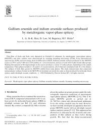
Example<br />
minimize log m ∑<br />
i=1<br />
exp(a T i x+b i)<br />
r<strong>and</strong>omly generated data with m = 2000, n = 1000, same fixed step size<br />
f(x (k) )−f ⋆<br />
|f ⋆ |<br />
10 0 gradient<br />
FISTA<br />
10 -1<br />
10 -2<br />
10 -3<br />
10 -4<br />
10 -5<br />
10 0 gradient<br />
FISTA<br />
10 -1<br />
10 -2<br />
10 -3<br />
10 -4<br />
10 -5<br />
10 -6 0 50 100 150 200<br />
FISTA is not a descent method<br />
k<br />
10 -6 0 50 100 150 200<br />
k<br />
Gradient methods 136
Dual methods<br />
<strong>Convex</strong> optimization — MLSS 2012<br />
• Lagrange duality<br />
• dual decomposition<br />
• dual proximal gradient method<br />
• multiplier methods
Dual function<br />
convex problem (with linear constraints for simplicity)<br />
minimize f(x)<br />
subject to Gx ≤ h<br />
Ax = b<br />
Lagrangian<br />
L(x,λ,ν) = f(x)+λ T (Gx−h)+ν T (Ax−b)<br />
dual function<br />
g(λ,ν) = inf<br />
x L(x,λ,ν)<br />
= −f ∗ (−G T λ−A T ν)−h T λ−b T ν<br />
f ∗ (y) = sup x (y T x−f(x)) is conjugate of f<br />
Dual methods 137
Dual problem<br />
maximize g(λ,ν)<br />
subject to λ ≥ 0<br />
a convex optimization problem in λ, ν<br />
duality theorem (p ⋆ is primal optimal value, d ⋆ is dual optimal value)<br />
• weak duality: p ⋆ ≥ d ⋆ (without exception)<br />
• strong duality: p ⋆ = d ⋆ if a constraint qualification holds<br />
(for example, primal problem is feasible <strong>and</strong> domf open)<br />
Dual methods 138
Norm approximation<br />
minimize ‖Ax−b‖<br />
reformulated problem<br />
minimize ‖y‖<br />
subject to y = Ax−b<br />
dual function<br />
(<br />
g(ν) = inf ‖y‖+ν T y −ν T Ax+b T ν )<br />
x,y<br />
{<br />
b<br />
=<br />
T ν A T ν = 0, ‖ν‖ ∗ ≤ 1<br />
−∞ otherwise<br />
dual problem<br />
maximize b T z<br />
subject to A T z = 0, ‖z‖ ∗ ≤ 1<br />
Dual methods 139
Karush-Kuhn-Tucker optimality conditions<br />
if strong duality holds, then x, λ, ν are optimal if <strong>and</strong> only if<br />
1. x is primal feasible<br />
x ∈ domf, Gx ≤ h, Ax = b<br />
2. λ ≥ 0<br />
3. complementary slackness holds<br />
λ T (h−Gx) = 0<br />
4. x minimizes L(x,λ,ν) = f(x)+λ T (Gx−h)+ν T (Ax−b)<br />
for differentiable f, condition 4 can be expressed as<br />
∇f(x)+G T λ+A T ν = 0<br />
Dual methods 140
Outline<br />
• Lagrange dual<br />
• dual decomposition<br />
• dual proximal gradient method<br />
• multiplier methods
Dual methods<br />
primal problem<br />
minimize f(x)<br />
subject to Gx ≤ h<br />
Ax = b<br />
dual problem<br />
maximize −h T λ−b T ν −f ∗ (−G T λ−A T ν)<br />
subject to λ ≥ 0<br />
possible advantages of solving the dual when using first-order methods<br />
• dual problem is unconstrained or has simple constraints<br />
• dual is differentiable<br />
• dual (almost) decomposes into smaller problems<br />
Dual methods 141
(Sub-)gradients of conjugate function<br />
f ∗ (y) = sup<br />
x<br />
(<br />
y T x−f(x) )<br />
• subgradient: x is a subgradient at y if it maximizes y T x−f(x)<br />
• if maximizing x is unique, then f ∗ is differentiable at y<br />
this is the case, for example, if f is strictly convex<br />
strongly convex function: f is strongly convex with modulus µ > 0 if<br />
f(x)− µ 2 xT x is convex<br />
implies that ∇f ∗ (x) is Lipschitz continuous with parameter 1/µ<br />
Dual methods 142
Dual gradient method<br />
primal problem with equality constraints <strong>and</strong> dual<br />
minimize f(x)<br />
subject to Ax = b<br />
dual ascent: use (sub-)gradient method to minimize<br />
−g(ν) = b T ν +f ∗ (−A T ν) = sup<br />
x<br />
(<br />
(b−Ax) T ν −f(x) )<br />
algorithm<br />
x = argmin<br />
ˆx<br />
ν + = ν +t(Ax−b)<br />
(<br />
f(ˆx)+ν T (Aˆx−b) )<br />
of interest if calculation of x is inexpensive (for example, separable)<br />
Dual methods 143
Dual decomposition<br />
convex problem with separable objective, coupling constraints<br />
minimize f 1 (x 1 )+f 2 (x 2 )<br />
subject to G 1 x 1 +G 2 x 2 ≤ h<br />
dual problem<br />
maximize −h T λ−f ∗ 1(−G T 1λ)−f ∗ 2(−G T 2λ)<br />
subject to λ ≥ 0<br />
• can be solved by (sub-)gradient projection if λ ≥ 0 is the only constraint<br />
• evaluating objective involves two independent minimizations<br />
f ∗ j(−G T j λ) = −inf<br />
x j<br />
(<br />
fj (x j )+λ T G j x j<br />
)<br />
minimizer x j gives subgradient −G j x j of f ∗ j (−GT j<br />
λ) with respect to λ<br />
Dual methods 144
dual subgradient projection method<br />
• solve two unconstrained (<strong>and</strong> independent) subproblems<br />
x j = argmin<br />
ˆx j<br />
(<br />
fj (ˆx j )+λ T G jˆx j<br />
)<br />
, j = 1,2<br />
• make projected subgradient update of λ<br />
λ + = (λ+t(G 1 x 1 +G 2 x 2 −h)) +<br />
interpretation: price coordination between two units in a system<br />
• constraints are limits on shared resources; λ i is price of resource i<br />
• dual update λ + i = (λ i −ts i ) + depends on slacks s = h−G 1 x 1 −G 2 x 2<br />
– increases price λ i if resource is over-utilized (s i < 0)<br />
– decreases price λ i if resource is under-utilized (s i > 0)<br />
– never lets prices get negative<br />
Dual methods 145
Outline<br />
• Lagrange dual<br />
• dual decomposition<br />
• dual proximal gradient method<br />
• multiplier methods
First-order dual methods<br />
minimize f(x)<br />
subject to Gx ≥ h<br />
Ax = b<br />
maximize −f ∗ (−G T λ−A T ν)<br />
subject to λ ≥ 0<br />
subgradient method: slow, step size selection difficult<br />
gradient method: faster, requires differentiable f ∗<br />
• in many applications f ∗ is not differentiable, or has nontrivial domain<br />
• f ∗ can be smoothed by adding a small strongly convex term to f<br />
proximal gradient method (this section): dual cost split in two terms<br />
• first term is differentiable<br />
• second term has an inexpensive prox-operator<br />
Dual methods 146
Composite structure in the dual<br />
primal problem with separable objective<br />
minimize f(x)+h(y)<br />
subject to Ax+By = b<br />
dual problem<br />
maximize −f ∗ (A T z)−h ∗ (B T z)+b T z<br />
has the composite structure required for the proximal gradient method if<br />
• f is strongly convex; hence ∇f ∗ is Lipschitz continuous<br />
• prox-operator of h ∗ (B T z) is cheap (closed form or simple algorithm)<br />
Dual methods 147
Regularized norm approximation<br />
minimize f(x)+‖Ax−b‖<br />
f strongly convex with modulus µ; ‖·‖ is any norm<br />
reformulated problem <strong>and</strong> dual<br />
minimize f(x)+‖y‖<br />
subject to y = Ax−b<br />
maximize b T z −f ∗ (A T z)<br />
subject to ‖z‖ ∗ ≤ 1<br />
• gradient of dual cost is Lipschitz continuous with parameter ‖A‖ 2 2/µ<br />
∇f ∗ (A T z) = argmin<br />
x<br />
(<br />
f(x)−z T Ax )<br />
• for most norms, projection on dual norm ball is inexpensive<br />
Dual methods 148
dual gradient projection algorithm for<br />
minimize f(x)+‖Ax−b‖<br />
choose initial z <strong>and</strong> repeat<br />
x = argmin<br />
ˆx<br />
(<br />
f(ˆx)−z T Aˆx )<br />
z + = P C (z +t(b−Ax))<br />
• P C is projection on C = {y | ‖y‖ ∗ ≤ 1}<br />
• step size t is constant or from backtracking line search<br />
• can use accelerated gradient projection algorithm (FISTA) for z-update<br />
• first step decouples if f is separable<br />
Dual methods 149
Outline<br />
• Lagrange dual<br />
• dual decomposition<br />
• dual proximal gradient method<br />
• multiplier methods
Moreau-Yosida smoothing of the dual<br />
dual of equality constrained problem<br />
maximize g(ν) = inf x<br />
(<br />
f(x)+ν T (Ax−b) )<br />
smoothed dual problem<br />
maximize g (t) (ν) = sup<br />
z<br />
• same solution as non-smoothed dual<br />
• equivalent expression (from duality)<br />
g (t) (ν) = inf<br />
x<br />
(<br />
g(z)− 1 )<br />
2t ‖z −ν‖2 2<br />
(<br />
f(x)+ν T (Ax−b)+ t )<br />
2 ‖Ax−b‖2 2<br />
∇g (t) (ν) = Ax−b with x the minimizer in the definition<br />
Dual methods 150
Augmented Lagrangian method<br />
algorithm: choose initial ν <strong>and</strong> repeat<br />
x = argmin<br />
ˆx<br />
L t (ˆx,ν)<br />
ν + = ν +t(Ax−b)<br />
• L t is the augmented Lagrangian (Lagrangian plus quadratic penalty)<br />
L t (x,ν) = f(x)+ν T (Ax−b)+ t 2 ‖Ax−b‖2 2<br />
• maximizes smoothed dual function g t via gradient method<br />
• can be extended to problems with inequality constraints<br />
Dual methods 151
Dual decomposition<br />
convex problem with separable objective<br />
minimize f(x)+h(y)<br />
subject to Ax+By = b<br />
augmented Lagrangian<br />
L t (x,y,ν) = f(x)+h(y)+ν T (Ax+By −b)+ t 2 ‖Ax+By −b‖2 2<br />
• difficulty: quadratic penalty destroys separability of Lagrangian<br />
• solution: replace minimization over (x,y) by alternating minimization<br />
Dual methods 152
Alternating direction method of multipliers<br />
apply one cycle of alternating minimization steps to augmented Lagrangian<br />
1. minimize augmented Lagrangian over x:<br />
x (k) = argmin<br />
x<br />
2. minimize augmented Lagrangian over y:<br />
y (k) = argmin<br />
y<br />
L t (x,y (k−1) ,ν (k−1) )<br />
L t (x (k) ,y,ν (k−1) )<br />
3. dual update:<br />
ν (k) := ν (k−1) +t<br />
( )<br />
Ax (k) +By (k) −b<br />
can be shown to converge under weak assumptions<br />
Dual methods 153
Example: regularized norm approximation<br />
f convex (not necessarily strongly)<br />
minimize f(x)+‖Ax−b‖<br />
reformulated problem<br />
minimize f(x)+‖y‖<br />
subject to y = Ax−b<br />
augmented Lagrangian<br />
L t (x,y,z) = f(x)+‖y‖+z T (y −Ax+b)+ t 2 ‖y −Ax+b‖2 2<br />
Dual methods 154
ADMM steps (with f(x) = ‖x−a‖ 2 2/2 as example)<br />
L t (x,y,z) = f(x)+‖y‖+z T (y −Ax+b)+ t 2 ‖y −Ax+b‖2 2<br />
1. minimization over x<br />
x := argmin<br />
ˆx<br />
L t (ˆx,y,ν) = (I +tA T A) −1 (a+A T (z +t(y −b))<br />
2. minimization over y via prox-operator of ‖·‖/t<br />
y := argmin<br />
ŷ<br />
L t (x,ŷ,z) = prox ‖·‖/t (Ax−b−(1/t)z)<br />
can be evaluated via projection on dual norm ball C = {u | ‖u‖ ∗ ≤ 1}<br />
3. dual update: z := z +t(y −Ax−b)<br />
cost per iteration dominated by linear equation in step 1<br />
Dual methods 155
Example: sparse covariance selection<br />
minimize tr(CX)−logdetX +‖X‖ 1<br />
variable X ∈ S n ; ‖X‖ 1 is sum of absolute values of X<br />
reformulation<br />
minimize tr(CX)−logdetX +‖Y‖ 1<br />
subject to X −Y = 0<br />
augmented Lagrangian<br />
L t (X,Y,Z)<br />
= tr(CX)−logdetX +‖Y‖ 1 +tr(Z(X −Y))+ t 2 ‖X −Y‖2 F<br />
Dual methods 156
ADMM steps: alternating minimization of augmented Lagrangian<br />
tr(CX)−logdetX +‖Y‖ 1 +tr(Z(X −Y))+ t 2 ‖X −Y‖2 F<br />
• minimization over X:<br />
X := argmin<br />
ˆX<br />
(<br />
−logdet ˆX + t 2 ‖ ˆX −Y + 1 t (C +Z)‖2 F<br />
solution follows from eigenvalue decomposition of Y −(1/t)(C +Z)<br />
• minimization over Y:<br />
Y := argmin<br />
Ŷ<br />
(<br />
‖Ŷ‖ 1+ t 2 ‖Ŷ −X − 1 )<br />
t Z‖2 F<br />
apply element-wise soft-thresholding to X −(1/t)Z<br />
• dual update Z := Z +t(X −Y)<br />
cost per iteration dominated by cost of eigenvalue decomposition<br />
)<br />
Dual methods 157
Douglas-Rachford splitting algorithm<br />
minimize g(x)+h(x)<br />
with g <strong>and</strong> h closed convex functions<br />
algorithm<br />
ˆx (k+1) = prox tg (x (k) −y (k) )<br />
x (k+1) = prox th (ˆx (k+1) +y (k) )<br />
y (k+1) = y (k) + ˆx (k+1) −x (k+1)<br />
• converges under weak conditions (existence of a solution)<br />
• useful when g <strong>and</strong> h have inexpensive prox-operators<br />
Dual methods 158
ADMM as Douglas-Rachford algorithm<br />
dual problem<br />
minimize f(x)+h(y)<br />
subject to Ax+By = b<br />
maximize b T z −f ∗ (A T z)−h ∗ (B T z)<br />
ADMM algorithm<br />
• split dual objective in two terms g 1 (z)+g 2 (z)<br />
g 1 (z) = b T z −f ∗ (A T z), g 2 (z)−h ∗ (B T z)<br />
• Douglas-Rachford algorithm applied to the dual gives ADMM<br />
Dual methods 159
Sources <strong>and</strong> references<br />
these lectures are based on the courses<br />
• EE364A (S. Boyd, Stanford), EE236B (<strong>UCLA</strong>), <strong>Convex</strong> <strong>Optimization</strong><br />
www.stanford.edu/class/ee364a<br />
www.ee.ucla.edu/ee236b/<br />
• EE236C (<strong>UCLA</strong>) <strong>Optimization</strong> Methods for Large-Scale Systems<br />
www.ee.ucla.edu/~v<strong>and</strong>enbe/ee236c<br />
• EE364B (S. Boyd, Stanford University) <strong>Convex</strong> <strong>Optimization</strong> II<br />
www.stanford.edu/class/ee364b<br />
see the websites for exp<strong>and</strong>ed notes, references to literature <strong>and</strong> software<br />
Dual methods 160