Assignment 7: Integration and ODEs Problem 1

CEE 3804: Computer Applications in Civil Engineering Spring 2010
Date Due: April 8, 2010 (Class Time)
Problem 1
Assignment 7: Integration and ODEs
Instructor: Trani
Steel is one of the most important materials used in Civil Engineering. A civil engineer wants to estimate the distribution of the
Modulus of Elasticity (Young’s modulus) for various specimens of steel beams received from a factory. The engineer collects data
and finds that the modulus of elasticity is normally distributed. The equation of the Probability Density Function (PDF) of the
Gaussian (or Normal) distribution is given in any statistics textbook and repeated here for completeness (http://en.wikipedia.org/
wiki/Normal_distribution).
−
1
f (x) =
σ 2π e
⎡ (x− µ )2 ⎤
⎢
⎣ 2σ 2 ⎥
⎦
where: x is the random variable in question (modulus of elasticity in psi) and µ and σ are the mean and standard deviation (in
psi) of the random phenomena modeled. After testing 100 samples, the engineer estimates the mean modulus of elasticity to be
2.856 e7 psi. The standard deviation is found to be 4.1e5.
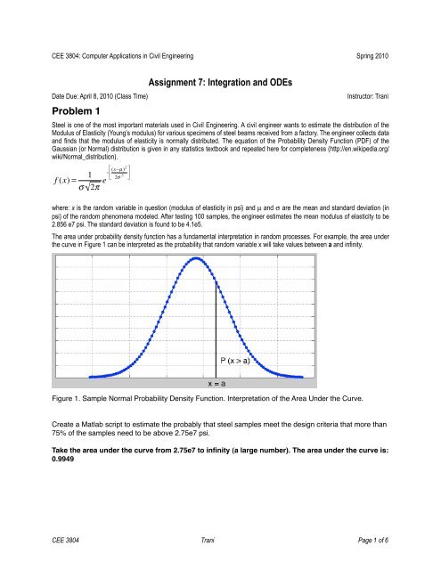
The area under probability density function has a fundamental interpretation in random processes. For example, the area under
the curve in Figure 1 can be interpreted as the probability that random variable x will take values between a and infinity.
Figure 1. Sample Normal Probability Density Function. Interpretation of the Area Under the Curve.
Create a Matlab script to estimate the probably that steel samples meet the design criteria that more than
75% of the samples need to be above 2.75e7 psi.
Take the area under the curve from 2.75e7 to infinity (a large number). The area under the curve is:
0.9949
CEE 3804 Trani Page 1 of 6

Task 4
Using your Matlab function and scripts, verify that the area under the Normal curve is equal to one.
Script to calculate area under the curve.
___________
% Normal Distribution Analysis
% A.A. Trani
% Function calls:
global MU SIGMA
% Define the parameter of the distribution (MU) and standard deviation (SIGMA)
MU = 2.856e7;
SIGMA = 4.1e5;
% Define upper and lower bounds to get a nice plot of the Gaussian PDF
npoints = 100;
parameter = 3.5;
low = MU - parameter*SIGMA;
high = MU + parameter* SIGMA;
interval = (high - low) / npoints;
ub = MU + parameter* SIGMA;
lb = 2.75e7;
CEE 3804 Trani Page 2 of 6

% Define random variable
x=low:interval:high;
% Define the function of the random variable x (PDF function)
fx = 1/(SIGMA * sqrt(2*pi)) * exp(-1/2 * ((x-MU)/SIGMA).^2 );
% Plot the random variable x versus the PDF function
plot(x,fx)
xlabel('Random variable - x')
ylabel('f(x)')
grid
% Compute area under the curve f(x) from -infinity to infinity
% Change the values of the last two arguments if you
% want another range of values
area=quad('normalg',lb,ub);
disp(' ')
disp([blanks(5),'Area under the Normal Distribution : '])
disp(' ')
disp([blanks(5),' P(x>0)=',num2str(area)])
disp(' ')
_____________
Function Normalg.m
____________
% Function to evaluate the area under the normal distribution
% Passes back a single argument containing f(x) for the normal PDF function
function f = normalg(x);
global MU SIGMA
f = 1./(SIGMA .* sqrt(2*pi)) .* exp(-1/2 .* ((x-MU)./SIGMA).^2 );
CEE 3804 Trani Page 3 of 6

Problems 2-3
The differential equation to predict the acceleration dv
dt
dv
dt = k 1 + k 2 v + k 3 v2
of a high-speed train is given by the formula:
where: k 1
, k 2
, and k 3
are coefficients of the high-speed train and v is the speed of the high-speed train (in meters/second) .
In the equation presented, the dimensions of the acceleration are m/s 2 . The values of the coefficients are: 0.39, -0.0033 and
-3.2e-5, respectively.
Solution:
dV
= k 1
+ k 2
V + k 3
V 2
dt
x 1
= speed
x 2
= position
xdot 2
= x 1
xdot 1
= k 1
+ k 2
V + k 3
V 2
The Matlab main script is:
__________________
% Main file to execute the equations of motion of the HS Train
% A. Trani
% Solution to a set of equations of the form:
%
% x(1) = speed (m/s)
% x(2) = position (m)
%
% xdot(2) = x(1);
% xdot(1) = k1 + k2 * x1 + k3 * x1^2
%
% subject to initial conditions:
%
% x (t=0) = xo
%
% where:
clear
CEE 3804 Trani Page 4 of 6

global k1 k2 k3
% Define the Initial Conditions of the Problem
xo = [0 0];
to = 0.0;
tf = 300;
% xo are the initial position and speed of the train
% to is the initial time to solve this equation
% tf is the final time (seconds)
% define m and b
k1 = 0.39; %
k2 = -0.0033; %
k3 = -3.2e-5; %
tspan =[to tf];
[t,x] = ode15s('trainProfile',tspan,xo);
% call ODE solver
% Plot the results of the numerical integration procedure
figure
plot(t,x(:,1),'o-r')
xlabel('Time (seconds)')
ylabel('Speed (m/s)')
grid
figure
plot(t,x(:,2),'^--k')
xlabel('Time (seconds)')
ylabel('Position (m)')
grid
___________
Function trainProfile.m
________________
% Two first-order DEQ to solve the train system
function xdot = trainProfile(t,x)
global k1 k2 k3
% define the rate equations of the train system
%
% x(1) = speed (m/s)
% x(2) = distance traveled (m)
% xdot(1) = rate of change of speed vs time = acceleration
CEE 3804 Trani Page 5 of 6

% xdot(2) = rate of change of distance vs time = speed
xdot(2) = x(1);
xdot(1) = k1 + k2 * x(1) + k3 * x(1).^2;
xdot = xdot';
The plots are shown below.
CEE 3804 Trani Page 6 of 6