Assignment 1: Matlab Practice

CEE 3604: Introduction to Transportation Engineering Fall 2009
Date Due: September 3, 2009
Assignment 1: Matlab Practice
Instructor: Trani
Problem 1
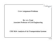
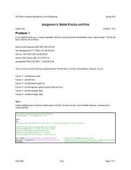
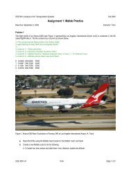
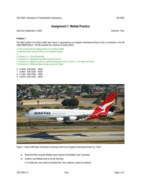
The flight profile of an Airbus A380 (see Figure 1) approaching Los Angeles International Airport (LAX) is contained in the file
called flightProfile.m. The file contains four columns as shown below.
% File containing the flight profile of an Airbus A380
% approaching runway 24R at Los Angeles airport
%
% Column 1 = Time (seconds)
% Column 2 = Distance traveled (nautical miles)
% Column 3 = Speed (knots or nautical miles per hour). A knot = 1.15 miles per hour
% Column 4 = Altitude above mean sea level (feet)
0 0.0000 249.0000 5500
1 0.0691 248.7528 5500
2 0.1381 248.7528 5500
3 0.2072 248.7528 5500
.....
Figure 1. Airbus A380 Near Touchdown to Runway 24R at Los Angeles International Airport (A. Trani).
a) Read the M-file using the Matlab import wizard or the Matlab “load” command
b) Create a new Matlab script to do the following:
b.1) Create four new vectors and label them: time, distance, speed and altitude.
CEE 3604 A1 Trani Page 1 of 3

.2) Insert the values of time, distance traveled, speed and altitude in the original file into each one of the vectors
created in step (b.1).
b.3) Plot distance traveled (in x-axis) vs speed (y-axis). Label axes and change default font sizes to size 16 for both x
and y labels. Change the color of the line to blue. Comment on the shape of the profile observed.
b.5) Plot distance traveled (in x-axis) vs altitude (y-axis). Label axes and change default font sizes to size 16 for both x
and y labels. Change the color of the line to red. Comment on the shape of the profile observed.
c) Estimate the average speed (in knots) for this flight profile from time = 0 to touchdown. The elevation of the airport is
127.11 feet above sea level. Show your procedure to estimate the average speed.
d) For safety reasons (due to wake vortex), aircraft approaching the same runway are kept 10 nautical miles behind the
A380. Find the number of Airbus A380s that could land in one hour on the same runway. This value is called the hourly
capacity of the runway.
_____________________________________________
Problem 2
The speed profile of a Toyota Camry traveling on an arterial road in the state of New Mexico is contained in the file called
gpsData.m. The file contains three columns as shown below.
% GPS car data collected in New Mexico
% Car = Toyota Camry (model 2001)
%
% Column 1 = Time of observation (seconds)
% Column 2 = Distance traveled (m)
% Column 3 = Speed (km/hr)
0 0 0
2 24.1 42.1
4 51.3 52.1
6 82.9 55.6
8 115.6 58.9
10 149.3 60.8
....
a) Import the data into Matlab using the import wizard or using the “load” command.
b) Create a Matlab script to plot the distance traveled by the car as a function of time (plot time in the x-axis). Label your
axes and place a descriptive title for this plot.
c) Plot the speed of the car in miles per hour (in y-axis) vs time (x- axis). Label the axes and add a title. Change the line
color to red and line width 3.
d) Find the average speed of the car through the complete speed profile.
e) Find the number of seconds the car spends at a red traffic light.
Problem 3
Data has been collected in California (Highway 101) using new speed sensors. A file called highwayData.m contains samples of
vehicle speed and highway density data for this problem. Traffic flow density and traffic flow speed are two key variables of
interest to transportation engineers to study the level of service offered by highway. The file contains four columns as shown
below.
% Traffic Flow Data
% Highway 101
%
% Column 1 = Density (veh/km-lane)
CEE 3604 A1 Trani Page 2 of 3

% Column 2 = Speed (km/hr)
% Column 3 = Flow (veh/hr per lane)
% Column 4 ignore for this problem
9.5 110 1044 106
7.8 109 853 128
9.3 109 1012 108
......
a) Use Matlab to plot the values of Density (x-axis) vs Speed (y-axis). Comment of the trend observed. Label the axes in the plot
and use a red marker “o” to indicate each data point in your plot.
b) Using the “Basic Fitting” capabilities in Matlab (look at the “Tools” pull down menu in your plot), fit a first degree polynomial to
the data. Indicate the equation of the polynomial and comment on how well the polynomial fits the data.
c) The “density” of the traffic on the highway is an indicator of the number of vehicles per kilometer (per lane) traveling on the
highway. If one night the traffic sensors detect 10 vehicles per kilometer, estimate the speed of the traffic flow (in km/hr).
Problem 4
An empirical formula used to estimate the thickness of an airport pavement is:
t =
where:
P
8.1CBR + A π
t is the design pavement thickness (in inches)
P is the equivalent single wheel load of the aircraft tires on the pavement (in pounds)
A is the single tire contact area (square inches)
CBR is the California Bearing Ratio (a dimensionless factor a function of the physical supporting properties of the soil)
a) Create a Matlab script to calculate parametrically the pavement thicknesses required to support an Airbus A380 with P =
60,000 lbs and A = 340 square inches for various values of CBR ranging from 10 to 50. In your calculations use vector
operations (read pages 7-14 in document matlab_matrices.pdf or http://128.173.204.63/courses/matlab/
matlab_matrices.pdf).
b) Plot the solutions obtained in part (a) and label accordingly.
CEE 3604 A1 Trani Page 3 of 3