An improved reproducing kernel particle method for nearly ...

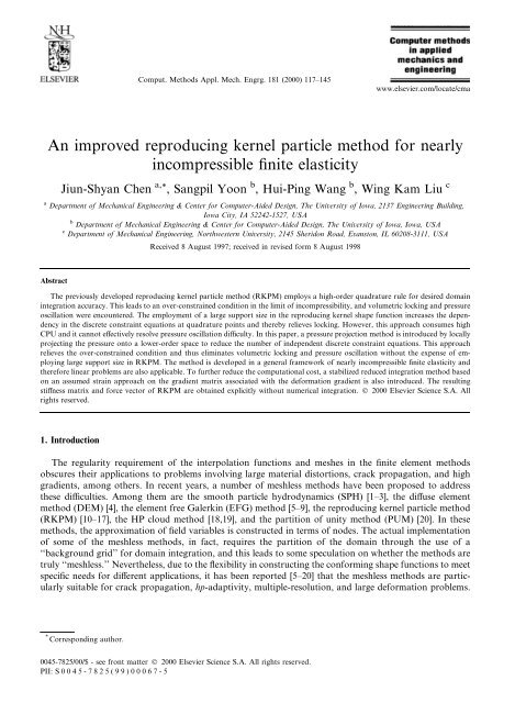
Comput. Methods Appl. Mech. Engrg. 181 (2000) 117±145 

www.elsevier.com/locate/cma 

An improved reproducing kernel particle method for nearly 

incompressible ®nite elasticity 

Jiun-Shyan Chen a, * 

, Sangpil Yoon b , Hui-Ping Wang b , Wing Kam Liu c 

a Department of Mechanical Engineering & Center for Computer-Aided Design, The University of Iowa, 2137 Engineering Building, 

Iowa City, IA 52242-1527, USA 

b Department of Mechanical Engineering & Center for Computer-Aided Design, The University of Iowa, Iowa, USA 

c Department of Mechanical Engineering, Northwestern University, 2145 Sheridon Road, Evanston, IL 60208-3111, USA 

Received 8 August 1997; received in revised form 8 August 1998 

Abstract 

The previously developed reproducing kernel particle method (RKPM) employs a high-order quadrature rule for desired domain 

integration accuracy. This leads to an over-constrained condition in the limit of incompressibility, and volumetric locking and pressure 

oscillation were encountered. The employment of a large support size in the reproducing kernel shape function increases the dependency 

in the discrete constraint equations at quadrature points and thereby relieves locking. However, this approach consumes high 

CPU and it cannot e€ectively resolve pressure oscillation diculty. In this paper, a pressure projection method is introduced by locally 

projecting the pressure onto a lower-order space to reduce the number of independent discrete constraint equations. This approach 

relieves the over-constrained condition and thus eliminates volumetric locking and pressure oscillation without the expense of employing 

large support size in RKPM. The method is developed in a general framework of nearly incompressible ®nite elasticity and 

therefore linear problems are also applicable. To further reduce the computational cost, a stabilized reduced integration method based 

on an assumed strain approach on the gradient matrix associated with the deformation gradient is also introduced. The resulting 

sti€ness matrix and force vector of RKPM are obtained explicitly without numerical integration. Ó 2000 Elsevier Science S.A. All 

rights reserved. 

1. Introduction 

The regularity requirement of the interpolation functions and meshes in the ®nite element methods 

obscures their applications to problems involving large material distortions, crack propagation, and high 

gradients, among others. In recent years, a number of meshless methods have been proposed to address 

these diculties. Among them are the smooth particle hydrodynamics (SPH) [1±3], the di€use element 

method (DEM) [4], the element free Galerkin (EFG) method [5±9], the reproducing kernel particle method 

(RKPM) [10±17], the HP cloud method [18,19], and the partition of unity method (PUM) [20]. In these 

methods, the approximation of ®eld variables is constructed in terms of nodes. The actual implementation 

of some of the meshless methods, in fact, requires the partition of the domain through the use of a 

``background grid'' for domain integration, and this leads to some speculation on whether the methods are 

truly ``meshless.'' Nevertheless, due to the ¯exibility in constructing the conforming shape functions to meet 

speci®c needs for di€erent applications, it has been reported [5±20] that the meshless methods are particularly 

suitable for crack propagation, hp-adaptivity, multiple-resolution, and large deformation problems. 

* Corresponding author. 

0045-7825/00/$ - see front matter Ó 2000 Elsevier Science S.A. All rights reserved. 

PII: S 0 0 4 5 - 7 8 2 5 ( 9 9 ) 0 0 067-5

118 J.-S. Chen et al. / Comput. Methods Appl. Mech. Engrg. 181 (2000) 117±145 

One of the major disadvantages of the meshless methods is its relatively high computational cost. 

The supports of the meshless shape functions usually cover more surrounding points than those in the 

®nite element methods. This requirement increases the number of numerical operations in the sti€ness 

matrix formation and assembly, and the resulting global sti€ness matrix has large bandwidth. The 

situation is more signi®cant when dealing with incompressible problems, in which suciently large 

support sizes need to be used in the meshless shape functions to avoid incompressible locking 

[5,6,15,16]. In meshless formulation, higher-order weight functions and kernel functions such as the 

exponential function, Gauss function, and the cubic B-spline function are usually used, and therefore 

higher-order 

p p 

Gauss 

 

integration is required. Belytschko et al. [5,6] suggested an integration order of 

… m ‡ 2† … m ‡ 2†, with m the number of points within the integration zone for two-dimensional 

problems using an exponential typed weight function. For a two-dimensional integration zone containing 

four points, for example, meshless methods require 4 4 quadrature points, whereas only 2 2 

quadrature points are needed in 4-node ®nite elements. Other numerical operations that consume additional 

CPU time in meshless computation are the imposition of the essential boundary conditions by 

the Lagrangian multiplier method [5] or the direct transformation method [15,16], and the construction 

of meshless shape functions. 

The incompressible locking in ®nite elements has been studied extensively and various methods have 

been proposed to resolve this diculty resulting from the over-constrained nature in the displacementbased 

®nite element methods. Among them are the Lagrange-multiplier-type mixed methods [21±28], the 

selective reduced integration method [29,30], the hourglass control method on under-integrated elements 

[31±33], the Taylor expansion method [34±36], the volumetric strain projection method [37], the pressure 

projection method [38±40], and the rank-one ®ltering method [41]. In the pressure projection method 

[38,39], the displacement-calculated pressure is projected onto a lower-order pressure space by a leastsquares 

projection at the element level. The resulting equilibrium equation is equivalent to the perturbed 

Lagrangian formulation [27,28]. With an appropriate decomposition of the strain energy density function, 

and a selection of particular pressure interpolation functions, a fairly simple pressure projection formulation 

was obtained and it can be easily implemented into displacement-based ®nite element code. The 

degeneration of the pressure projection method to linear elasticity leads to the well known mean dilatation 

[42] and selective reduced integration [30] methods. The Taylor expansion approach is based on the assumed 

strain method [34±36], in which the assumed strain ®eld is obtained by the Taylor expansion of the 

displacement gradient matrix. The resulting sti€ness matrix and force vector can be expressed explicitly by 

one-point quadrature terms and their stabilization. 

In this paper, it is shown that the fully integrated RKPM is severely over-constrained in nearly incompressible 

problems, and a pressure projection method is developed to reduce the independent discrete 

constrained equations. A stabilized reduced integration method is also introduced to further reduce the 

computational e€ort in RKPM. 

The meshless shape functions developed from RKPM are reviewed in Section 2. Section 3 discusses the 

pressure projection method for RKPM ®nite elastic formulation. In Section 4, the RKPM formulation is 

further simpli®ed by introducing a Taylor series expansion of the gradient matrix on the selected terms of 

sti€ness matrix and force vector. Several linear and nonlinear problems are analyzed to verify the performance 

of the proposed method in Section 5, and conclusions are given in Section 6. 

2. Overview of reproducing kernel particle method 

2.1. Reproducing kernel approximation 

With no loss of generality, in this section we shall use the following notations: x ‰x 1 ; x 2 ; x 3 Š, 

y ‰y 1 ; y 2 ; y 3 Š, and dy dy 1 dy 2 dy 3 . The kernel estimate was ®rst introduced to the SPH [1±3], in which the 

kernel estimate of a function u…x† is 

Z 

u K …x† ˆ U a …x y†u…y† dy; 

…1† 

X

where u K …x† is the kernel estimate of u…x†, and U a …x y† the kernel function with support measure of a. 

The kernel function U a …x y† is a positive function with the following properties: 

Z 

U a …x y† dy ˆ 1; 

…2† 

X 

u K …x† ! u…x† as a ! 0: …3† 

The imposition of Eq. (2) is in fact the zeroth order consistency condition. Eq. (2), however, does not assure 

the consistency condition in the discrete form. To further restore the higher-order consistency conditions of 

the kernel estimate, Liu et al. [10] proposed a reproducing kernel approximation by introducing a correction 

function to the kernel estimate 

Z 

u R …x† ˆ C…x; x y†U a …x y†u…y† dy; 

…4† 

X 

J.-S. Chen et al. / Comput. Methods Appl. Mech. Engrg. 181 (2000) 117±145 119 

where u R …x† is the ``reproduced'' function of u…x†, and Eq. (4) is called the reproducing equation. The 

function C…x; x y† is the correction function de®ned by 

C…x; x y† ˆ b T …x†H…x y†; 

…5† 

where H…x y† is the vector of monomial basis functions, 

H T …x y† ˆ ‰1; x 1 y 1 ; x 2 y 2 ; x 3 y 3 ; …x 1 y 1 † 2 ; . . . ; …x 3 y 3 † N Š; 

b T …x† ˆ ‰b 0 …x†; b 1 …x†; . . .Š 

…6† 

…7† 

and b i …x†Õs are determined by imposing the following Nth order completeness requirement, i.e., if u…x† is a 

Nth order monomial, then we require 

Z 

u R …x† ˆ u…x† ˆ C…x; x y†U a …x y†u…y† dy: 

…8† 

X 

If u…x† is an Nth order monomial, one can express u…y† in terms of an Nth order Taylor expansion of x in 

Eq. (8) to yield 

u…y† ˆ u…x† ‡ ou…x† 

ox 1 

where 

 

w…x† T ˆ 

u…x†; ou…x† 

ox 1 

…y 1 x 1 † ‡ ou…x† …y 2 x 2 † ‡ ou…x† …y 3 x 3 † ‡ ˆ w…x† T H…x y†; …9† 

ox 2 

ox 3 

; ou…x† 

ox 2 

; ou…x† ; 

ox 3 

 

…10† 

and one can also express u…x† by 

u…x† ˆ w T …x†H…0†: 

…11† 

Substituting Eqs. (9) and (11) into Eq. (8) yields 

w…x† T ‰H…0† M…x†b…x†Š ˆ 0; 

where 

Z 

M…x† ˆ H…x y†H T …x y†U a …x y† dy: 

X 

Since u…x† is an arbitrary Nth order monomial, Eq. (12) implies 

b…x† ˆ M…x† 1 H…0† 

…12† 

…13† 

…14†


and 

C…x; x y† ˆ H T …0†M 1 …x†H…x y†: 

…15† 

Introducing Eq. (15) into Eq. (4) leads to the following reproducing kernel approximation 

Z 

Z 

u R …x† ˆ C…x; x y†U a …x; y†u…y† dy ˆ H T …0†M 1 …x† H…x y†U a …x y†u…y† dy: 

X 

Eq. (16) can be recast into the following form 

Z 

u R …x† ˆ U a …x; x y†u…y† dy; 

X 

where U a …x; x y† ˆ C…x; x y†U a …x y† is called the reproduced kernel. Since Eq. (17) exactly reproduces 

Nth order mononomials, the method ful®lls the Nth order consistency conditions, i.e., 

Z 

U a …x; x y†y l 1 ym 2 yn 3 dy ˆ xl 1 xm 2 xn 3 

for l ‡ m ‡ n ˆ 0; . . . ; N: …18† 

X 

X 

…16† 

…17† 

2.2. Discretization of reproducing kernel approximation 

Suppose that the domain X is discretized by a set of nodes fx 1 ; . . . ; x NP g, where x I is the location of node 

I, and NP the total number of points (nodes). By the use of a simple trapezoidal rule, Eq. (17) is discretized 

into 

u h …x† ˆ XNP 

C…x; x x I †U a …x x I † d I DV I ; 

Iˆ1 

…19† 

where U a …x x I † is the multi-dimensional kernel function that can be formed by taking the product of the 

one-dimensional kernel functions to yield 

U a …x x I † ˆ 1 

/ 

x 

1 x 1I 

/ x 

2 x 2I 

/ x 

3 x 3I 

; …20† 

a 1 a 2 a 3 a 1 a 2 a 3 

where a 1 , a 2 , and a 3 are measures of support in x 1 , x 2 , and x 3 directions, respectively, and this kernel 

function has rectangular (or brick) support. An alternative multi-dimensional kernel function with circular 

(or spherical) support is constructed by 

U a …x x I † ˆ 1 

a / 

 

kx x I k 

a 

 

: …21† 

An example of the one-dimensional kernel function is a cubic B-spline function: 

8 

2 

4jz 

3 j2 ‡ 4jzj 3 for 0 6 jzj 6 >< 

1 2 

/…z† ˆ 4 

4jzj 

‡ 4jz 

3 j2 4 jz 

3 j3 1 

for < jzj 

6 1 : …22† 

2 

>: 

0 otherwise 

The support of U a …x x I †, x I a 6 x 6 x I ‡ a, is centered at the point x I , and the size of the support is 

measured by the parameter a. 

In a multi-dimensional case, the determination of a volume associates with each node I, DV I , is not a 

straightforward task. Since the main purpose of this discretization is only to develop shape functions, we 

can simply set DV I to be unity 


C…x; x x I †U a …x x I † d I : 

Iˆ1 

…23†


Note that the correction function C…x; x x I † was determined previously from the completeness requirement 

of a continuous reproducing equation of Eq. (8). With the discretization of the reproducing equation, 

we shall re-impose the completeness requirement on Eq. (23) following the same procedures as were previously 

discussed to obtain: 

C…x; x x I † ˆ H T …0†M 1 …x†H…x x I †; 

…24† 

M…x† ˆ XNP 

H…x x I †H T …x x I †U a …x x I †: 

Iˆ1 

Eq. (23) can be expressed in the following form: 


W I …x† d I ; 

Iˆ1 

W I …x† ˆ C…x; x x I †U a …x x I †: 

…25† 

…26† 

…27† 

The function W I …x† is interpreted as the particle or meshless shape function of node I, and d I is the 

associated coef®cient of approximation. Since W I …x† is constructed based on the monomial basis functions 

and the kernel function U a …x x I †, the support of W I …x† is the same as the support of U a …x x I †. Further, 

the order of differentiability of W I …x† is also identical to that of U a …x x I † as discussed in [15]. Since the 

reproducing kernel shape functions satisfy the discrete completeness requirement, they meet the following 

consistency conditions 

X NP 

Iˆ1 

W I …x†x l 1I xm 2I xn 3I ˆ xl 1 xm 2 xn 3 

; l ‡ m ‡ n ˆ 0; . . . ; N: …28† 

It should be noted that, in general, the shape functions do not bear the Kronecker delta properties, i.e., 

W I …x J † 6ˆ d IJ . Therefore, for general function u…x† that is not a monomial, d I in Eq. (26) is not the nodal 

value of u…x†. This leads to some complication in imposing the essential boundary conditions in the 

meshless methods. Additional development such as the Lagrange multiplier method [5], the transformation 

method [15,16], or the singular kernel method [9] is required to impose the essential boundary conditions. 

3. Pressure projection 

3.1. Fundamental diculties in RKPM discretization of nearly incompressible ®nite elasticity 

For elastic materials that are nearly incompressible, the strain energy density W which can be expressed 

by the three invariants of strain, is penalized in the following form [25,27,28] 

W …I 1 ; I 2 ; J† ˆ W …I 1 J 2=3 ; I 2 J 4=3 † ‡ k ~w…J† 

and the corresponding potential energy is 

Z 

P ˆ ‰W …I 1 J 2=3 ; I 2 J 4=3 † ‡ k ~w…J†Š dX W ext ; 

X X 

…29† 

…30† 

where W is the distortional strain energy density, k ~w…J† the dilatational strain energy density, k is a penalty 

to impose incompressibility, J ˆ I 1=2 

3 

the volume ratio, I 1 ; I 2 ; I 3 are the three invariants of the Green deformation 

tensor, X X the domain of the original con®guration of the material, and W ext is the external 

energy. The stress-strain relation of the material is 

S ij ˆ oW ; 

…31† 

oE ij


where S is the second Piola±Kirchho€ stress, and E is the Green Lagrangian strain. By using the relation 

between the second Piola±Kirchho€ stress and the Cauchy stress, the pressure (trace of Cauchy stress) is 

obtained by [38] 

P ˆ k ~w 0 …J†: 

…32† 

A commonly used ~w function is [38]: 

~w…J† ˆ 1 

2 …J 1†2 …33† 

and the corresponding pressure equation is 

P ˆ k…J 1†: 

…34† 

By introducing the Galerkin approximation of the variation of the potential energy in Eq. (30), and 

approximating displacements by the reproducing kernel shape functions, the RKPM discrete equations can 

be obtained by [16]. As reported in [16], however, a volumetric locking exists unless a relatively large 

support size of the reproducing kernel shape function is used in the RKPM discretization. 

We introduce the method of constraint count [43] to study the ability of RKPM to perform well in nearly 

incompressible media. A discrete constraint ratio r c is de®ned by the ratio between the number of discrete 

equilibrium equations N eq and the number of independent constraint equations N c . We want the discrete 

constraint ratio r c to go toward the number of equilibrium equations divided by the number of incompressibility 

conditions in the continuum system when the number of discrete nodes approaches in®nity. 

Therefore the desired discrete constraint ratio in two-dimension is two. Let us introduce a rectangular 

domain partitioned into n integration zones 

p 

per 

 

side, and 

p 

each integration zone contains m nodes as shown 

in Fig. 1. Using an integration order of … m ‡ 2† … m ‡ 2† [5], the pressure equation obtained from 

Eq. (34) is computed at each integration point x l 

p 

P…x l † ˆ k…J…x l † 1† for l ˆ 1; . . . ; … m ‡ 2† 2 : …35† 

As the material behavior goes toward incompressible, for a bounded P the following incompressibility 

constraints are imposed at the integration points 

p 

2 

J…x l † 1 0 for l ˆ 1; . . . ; … m ‡ 2† …36† 

Fig. 1. Standard RKPM discretization.

or the linearized form 

p 

J…x l †Du i;i …x l † 0 ! Du i;i …x l † 0 for l ˆ 1; . . . ; … m ‡ 2† 2 : …37† 

p 

Note that the … m ‡ 2† 2 constraint equations in each integration zone are not necessarily linearly independent. 

If dependency exists, for a two-dimensional RKPM discretization the discrete constraint ratio is 

p 

2 

N eq 2‰n… m 1† ‡ 1Š 

r c ˆ lim ˆ lim 

n!1 N c n!1 

 

n 2 ‰… 

p m ‡ 2† 2 N d Š ‡ nb ˆ 2… p 2 

m 1† 

p ; m P 3; …38† 

… m ‡ 2† 2 N d 

where N d is the number of dependent incompressibility constraints in one integration zone, and this dependency 

is in¯uenced by the order and the support size of reproducing kernel shape functions. For the 

integration zones that are close to the boundary, the number of independent constraints is di€erent from 

those of the interior zones, and the di€erence is lumped into nb in Eq. (38). Since nb is only linearly 

proportional to n, it has no in¯uence on r c . If shape functions are monomials, it is easier to estimate N c 

directly. In a four-node ®nite element discretization for example, each integration point is covered by only 

four bilinear shape functions. Since 1; x; y; xy are independent monomials, the derivatives of displacement 

are represented by linear functions, and hence the total of independent constraints is N c ˆ 3n 2 , and this leads 

to a discrete constraint ratio of 

r c ˆ 2 < 2: …39† 

3 

This constraint ratio for a bilinear ®nite element is solely related to the order of bilinear ®nite element 

shape functions unless a one-point quadrature rule is used, which increases the constraint ratio to r c ˆ 2 

since N c ˆ n 2 . 

In RKPM discretization, the shape functions are generally not monomials. The number of independent 

constraints is then determined by the order of quadrature rule and the number of shape functions that cover 

each integration point. The number of shape functions that cover each integration point is directly related 

to the support size of shape functions. In a typical domain partitioning using a 4-node integration zone with 

4 4 integration order, the constraint ratio is: 

2 

r c ˆ ; …40† 

16 N d 

where N d is related to the support size. One can see that if no dependency in the incompressibility constraints 

exists, N d ˆ 0 results in a very low discrete constraint ratio 

r c ˆ 1 2: …41† 

8 

This causes a severe locking and a pressure oscillation, and therefore an increase of dependency in the 

constraint equations is necessary in RKPM discretization. One way to increase the dependency in the 

constraint equations is to enlarge the support size of reproducing kernel shape functions. As the kernel 

support size is enlarged, the number of reproducing kernel shape functions that cover each integration zone 

increases proportionally. This results in an increase of N d , and consequently r c increases and locking is 

reduced. This approach, however, signi®cantly raises the computational e€ort. One other approach is to let 

m ! 1 to yield lim m!1 r c ˆ 2 according to Eq. (38), but the method is practically useless. 

3.2. Pressure projection 


In this work, we reduce the independent constraint equations in each integration zone by projecting 

displacement calculated pressure (Eq. (34)) onto a lower-order space using a pressure projection method 

proposed by Chen et al. [38]. The lower-order approximation of pressure is performed locally by introducing 

a least-squares based projection on the displacement calculated pressure onto a pressure space 

spanned by a set of functions Q ˆ fQ 1 …x†; Q 2 …x†; . . . ; Q n …x†g within each zone of integration X s X 

. That is, 

determine p s ˆ ‰p1 s; ps 2 ; . . . ; ps n ŠT to minimize


w…p s † ˆ kk…J 

1† Qp s k 2 L 2 …X s X 

†; …42† 

where kk 2 L 2 …X s X † is the L 2 norm in the integration zone X s X 

. Note that the selection of pressure basis functions 

p 

Q should be based on Eq. (38) such that N c ! n 2 … m 1† 2 . The minimization of w…p s † leads to 

M s p s ˆ Z s ; 

where 

Z 

M s ˆ Q T Q dX; 

X s X 

Z 

Z s ˆ Q T k…J 1† dX 

X s X 

…43† 

…44† 

…45† 

and the projected hydrostatic pressure P s in X s X is 

P s Qp s ˆ QM s1 Z s : 

…46† 

In Eq. (46), the displacement calculated pressure k…J 1† is projected onto a space spanfQ i …x†g n iˆ1 . 

3.3. Incremental equation 

The variation of the potential energy in ®nite elasticity according to Eq. (30) is 

Z 

Z 

dP ˆ dF ij r ij dX ‡ dF ij ~r ij …P† dX dW ext 

X X X X 

…47† 

and the linearization is 

Z 

DdP ˆ dF ij ‰ T ijkl ‡ T ~ ijkl …P†ŠDF kl dX ‡ 

X X 

Z 

Z 

dF ij ‰ D ijkl ‡ ~D 1 ijkl …P†ŠDF kl dX 

X X 

‡ dF ij F 1 

ji 

JDP dX DdW ext ; 

X X 

…48† 

where 

r ij ˆ o W 

oF ij 

ˆ F mi 

S mj ; 

S ij ˆ o W 

oE ij 

; 

…49† 

~r ij ˆ k o ~w 

oF ij 

ˆ F mi 

~S mj ; ~S ij ˆ k o ~w 

oE ij 

; 

…50† 

DP ˆ kJF 1 

lk DF kl; …51† 

where F is the deformation gradient, r and ~r are the distortional and dilatational parts of ®rst Piola± 

Kirchho€ stress, respectively, and S and S ~ are the distortional and dilatational parts of the second Piola± 

Kirchho€ stress, respectively. The explicit expressions of S ij ; ~S ij ; D ijkl ; ~D 1 ijkl ; ~D 2 ijkl ; T ijkl ; ~T ijkl are listed in 

Appendix A. 

For the Galerkin approximation of Eq. (48), we further consider a local least-squares based projection of 

the pressure increment DP ˆ kJFkl 

1 DF kl in each integration zone X s X , by determining ^ps ˆ ‰^p 

1 s; ^ps 2 ; . . . ; ^ps n ŠT to 

minimize 

 

^w…^p s † ˆ kJF 1 Q^p s 

2 

…52† 

lk 

DF kl 

L 2 …X s X † :

The minimization of ^W…^p s † leads to 


^p s ˆ kM s1 L s Dd s ; 

where 

Z 

L s ˆ Q T gB dX; 

X s X 

…53† 

…54† 

g is the row vector form of JFij 

1 

increment, DP s , is obtained by 

and B the gradient matrix of deformation gradient. The projected pressure 

DP s Q^p s ˆ QM s1 L s Dd s : 

…55† 

By substituting Eqs. (46) and (55) into Eqs. (47) and (48) and introducing the RKPM displacement shape 

functions and domain discretization, the following incremental equation is obtained 

… K ‡ ~ K ‡ ~ K † m‡1 

n‡1 Dd ˆ … f ext ‡ ~ f ext † n‡1 

…f int † m n‡1 ; …56† 

where n is the load step counter and m the iteration counter. The stiffness term K IJ in Eq. (56) is related to 

the distortional energy that is independent to the pressure projection, 

Z 

K s IJ ˆ B T I … T ‡ D†B J dX; 

…57† 

X s X 

where the notation …† s IJ 

denotes the sti€ness matrices associated with particle I; J integrate over the integration 

zone X s X . The sti€ness matrix K ~ in Eq. (56) is related to the dilatational energy with pressure 

projected onto spanfQ i …x†g n iˆ1 

Z 

… K ~ † s IJ ˆ B T I ‰~ T…P s † ‡ D ~ 1 …P s †ŠB J dX: 

…58† 

X s X 

This sti€ness matrix contains the projected pressure. The third sti€ness term in Eq. (56) is the dilatational 

sti€ness associated with the projection of pressure increment: 

… ~ K † s IJ ˆ kLsT I 

M s1 L s J ; 

Z 

L s I ˆ 

X s X 

Q T gB I dX: 

…59† 

…60† 

Similarly, the internal force vector is also separated into f int and f ~ int . The internal force vector f int is related 

to the distortional energy that is independent of the pressure 

Z 

… f int † s I ˆ r dX; 

…61† 

X s X 

B T I 

where …† s I 

denotes the force vector associated with particle I integrate over the integration zone X s X . The 

second force vector in Eq. (56) is related to the dilatational energy 

Z 

… f ~ int † s I ˆ B T I ~r…P s † dX: 

…62† 

X s X 

This internal force vector contains the projected pressure. The matrices T, T, ~ D, D ~ 1 and Bdd are the matrix 

forms of d ik 

S jl , d ik 

~S jl , D ijkl , ~D 1 ijkl and dF ij, respectively, r and ~r are the vector form of r ij and ~r ij . The 

functions ~r ij , ~T ijkl and ~D 1 ijkl 

contain pressure that is calculated using the pressure projection equations. Note 

that one can also consider an incremental pressure equation by the linearization of Eq. (43). In this case, a 

pressure residual needs to be added consistently in Eqs. (53), (55) and (56).


3.4. Pressure projection for the most severe over-constrained condition 

Eq. (38) indicates that the most severe over-constrained condition in RKPM discretization is when only 

three or four nodes are included in each integration zone and when small kernel support size is used 

(N d 0). Under this condition, any pressure ®eld higher than a constant ®eld results in a very low discrete 

constraint ratio. For instance, a linear pressure ®eld leads to r c ˆ 1=3 and 2=3 for m ˆ 3 and 4, respectively. 

A basic 3-node integration unit X s X with centroid X s is shown in Fig. 2. Within each basic integration 

unit, the pressure is projected onto a constant ®eld, and the pressure projection equations reduce to 

P s ˆ k R …J 1† dX 

X s X 

; …63† 

A s 

DP s ˆ k R gB dX 

X s X 

Dd; …64† 

A s 

where A s is the area of X s X 

. Note that with constant pressure projection, the constraint count for a 3-node 

integration zone increases from 1/3 to 1, and for a 4-node integration zone it increases from 2/3 to 2. Using 

Eq. (64), the dilatational sti€ness matrix K ~ becomes 

Z ! Z ! 

… K ~ † s IJ ˆ B T kAs1 

I gT dX gB J dX : …65† 

X s X 

X s X 

If one further employs one-point integration to form Z s and L s , then the pressure projection equations 

reduce to following form: 

P s ˆ k‰J…X s † 1Š; 

DP s ˆ k…gB†j …X s ;Y s † Dd: 

…66† 

…67† 

Note that all the reproducing kernel shape functions that cover X s ˆ …X s ; Y s †, both inside and outside of 

X s X , contribute to the calculation of projected pressure P s . The dilatational sti€ness K also reduces to the 

following form 

Fig. 2. Pressure projection location in a triangular integration zone.


… ~ K † s IJ ˆ kAs …B T I gT gB J † 

…X s ;Y s † : 

…68† 

3.5. Degeneration to linear elasticity 

The pressure projection formulation can be degenerated to linear elasticity by setting F ij ! d ij to result 

in: 

T ijkl ˆ ~T ijkl ˆ ~D 1 ijkl ˆ 0; 

…69† 

D ijkl ˆ C ijkl ˆ C 1 ijkl ‡ C 2 ijkl ˆ 2 

3 …A 10 ‡ A 01 †‰3…d ik d jl ‡ d il d jk † 2d ij d kl Š: …70† 

In linear elasticity, the shear modulus can be related to A 10 and A 01 by 

 

l ˆ 2 

oW 

oI 1 

‡ oW 

ˆ 2…A 10 ‡ A 01 † 

oI 2 

I1ˆI 2ˆ3 

and thus 

 

C ijkl ˆ l …d ik d jl ‡ d il d jk † 2 3 d ijd kl 

: …72† 

…71† 

The pressure projection sti€ness matrix degenerates to 

Z 

K s IJ ˆ B T CB dX ‡ kA s …B T I gT gB J † : …X s ;Y s † 

X s X 

…73† 

Further reduction of g to g ˆ ‰1; 1; 1; 0; 0; 0Š, and taking the bulk modulus k ˆ k ‡ 2=3l, Eq. (73) can be 

rearranged as 

Z 

 

K s IJ ˆ B T I 

CB J dX ‡ k ‡ 2 …A 

3 l s b T I b J† ; …74† 

…X s ;Y s † 

X s X 

where 

b I ˆ ‰W I;X ; W I;Y Š: 

…75† 

4. Stabilized reduced integration 

4.1. Finite elasticity 

The computational eciency of RKPM can be further improved by introducing a stabilized reduced 

integration method for the construction of the sti€ness matrix and force vector. It has been discussed by 

Simo and Hughes [44], that if a certain orthogonality condition exists between the stress ®eld, strain ®eld, 

and displacement gradient in the Hu-Washizu variational principle, a single-®eld variational principle with 

strain as the independent variable can be obtained. Liu et al. [34] then introduced an assumed strain in the 

following form 

e ˆ Bd; 

where the assumed strain matrix B is the Taylor expansion of the displacement gradient matrix formulated 

in the natural coordinate. In meshless formulation, since the reproducing kernel shape functions are 

constructed at the global Cartesian coordinate, we introduce the following assumed deformation gradient 

®eld in the integration zone X s X : 

…76†


dF ˆ Bdd; DF ˆ BDd; …77† 

B I …X ; Y † ˆ B I j …X s ;Y s † ‡ …X X s †B I;X j ‡ …Y Y s …X s ;Y s † 

†B I;X j …X s ;Y s † 

for …X ; Y † 2 X s X ; …78† 

where …X s ; Y s † is the centroid of X s X as shown in Fig. 1. By replacing B I by B I of Eq. (78) in Eqs. (57) and 

(58), and further evaluating D , T, D, ~ and T ~ at …X s ; Y s † for …X ; Y † 2 X s X 

, one can obtain the following 

sti€ness matrices associated with the integration zone X s X : 

… K† s IJ ˆAs ‰B T I … T ‡ D†B J Š ‡ m s 

…X s ;Y s XX ‰BT I; 

† X 

… T ‡ D†B J;X Š ‡ m s 

…X s ;Y s YY ‰BT I; 

† Y 

… T ‡ D†B J;Y Š …X s ;Y s † 

‡ m s XY ‰BT I; X 

… T ‡ D†B J;Y ‡ B T I; Y 

… T ‡ D†B J;X Š ‡ K s 

…X s ;Y s IJ ; …79† 

† 

… K† ~ s IJ ˆ … K ~ † s IJ ‡ … K ~ † s IJ 

ˆ A s ‰B T I …~ T ‡ D ~ 1 †B J Š ‡ m s 


† X 

… T ~ ‡ D ~ 1 †B J;X Š ‡ m s 


† Y 

… T ~ ‡ D ~ 1 †B J;Y Š …X s ;Y s † 


… T ~ ‡ D ~ 1 †B J;Y ‡ B T I; Y 

… T ~ ‡ D ~ 1 †B J;X Š ‡ kA s …B T 

…X s ;Y s I gT gB J † ‡ 

† …X 

K ~ s s ;Y s † IJ : …80a† 

The ®rst term and the second last term in Eq. (80a) can be combined to yield 

… K† ~ s IJ ˆ As ‰B T I …~ T ‡ D ~ 1 ‡ D ~ 2 †B J Š ‡ m s 


† X 

… T ~ ‡ D ~ 1 †B J;X Š ‡ m s 


† Y 

… T ~ ‡ D ~ 1 †B J;Y Š …X s ;Y s † 


… T ~ ‡ D ~ 1 †B J;Y ‡ B T I; Y 

… T ~ ‡ D ~ 1 †B J;X Š ‡ K ~ s 

…X s ;Y s IJ ; …80b† 

† 

where A s is the area of X s X , and ms XX , ms YY and ms XY are the second area moments of Xs X 

that can be directly 

related to or approximated by the moment of inertia IXX s , I YY s , and I XY s of Xs X 

as shown in Table 1. Note 

that the moment of inertia can be obtained analytically without numerical integration. The matrices K s IJ 

and K ~ s IJ 

that contain the ®rst moments vanish in plane-strain case, and are nonzero for an axisymmetric 

problem: 

K s IJ ˆ ms X ‰BT I; X 

… T ‡ D†B J ‡ B T I … T ‡ D†B J;X Š ‡ m s 

…X s ;Y s Y ‰BT I; 

† Y 

… T ‡ D†B J ‡ B T I … T ‡ D†B J;Y Š …81† 

…X s ;Y †; s 

~K s IJ ˆ ms X ‰BT I; X 

… T ~ ‡ D ~ 1 †B J ‡ B T I …~ T ‡ D ~ 1 †B J;X Š ‡ m s 


† Y 

… T ~ ‡ D ~ 1 †B J ‡ B T I …~ T ‡ D ~ 1 †B J;Y Š …X s ;Y †: 

s 

By combining Eqs. (79) and (80b), we obtain the following explicit tangential sti€ness matrix for ®nite 

elasticity 

…82† 

…K† s IJ ˆ … K† s IJ ‡ … ~K † s IJ ‡ … ~K † s IJ ˆ …K 0† s IJ ‡ …K stab† s IJ ; 

…83† 

where 

…K 0 † s IJ ˆ Ak ‰B T I …D ‡ T†B JŠ 

…X s ;Y s † ; 

…84† 

…K stab † s IJ ˆ ms XX ‰BT I; X 

…D ‡ T†B J;X Š ‡ m s 


† Y 

…D ‡ T†B J;Y Š …X s ;Y s † 


…D ‡ T†B J;Y ‡ B T I; Y 

…D ‡ T†B J;X Š ‡ K s 

…X s ;Y s IJ ; …85† 

†


Table 1 

Area moments for plane-strain and axisymmetric cases 

Plane-strain 

Axisymmetric 

m s X 

0 Z 

m s Y 

0 Z 

m s XX 

m s YY 

m s XY 

Z 

Z 

Z 

X s X 

X s X 

X s X 

…X X s † 2 dX ˆ I s XX 

…Y Y s † 2 dX ˆ I s YY 

…X X s †…Y Y s † dX ˆ I s XY 

Z 

Z 

Z 

Z 

X s X 

X K X 

X S X 

X s X 

X s X 

X s X 

Z 

…X X s †X dX ˆ …X X s † 2 dX ˆ I s XX 

X s X 

Z 

…Y Y S †X dX ˆ …X X S †…Y Y S †dX ˆ I S XY 

X K X 

Z 

…Y Y S †X dX ˆ …X X S †…Y Y S † dX ˆ I S XY 

X S X 

…X X s † 2 X dX X s Z 

…Y Y s † 2 X dX X s Z 

X s X 

X s X 

…X X s †…Y Y s †X dX X s I s XY 

…X X s † 2 dX ˆ X s I s XX 

…Y Y s † 2 dX ˆ X s I s YY 

K s IJ ˆ ms X ‰BT I; X 

…D ‡ T†B J ‡ B T I …D ‡ T†B J;X Š ‡ m s 


† Y 

…D ‡ T†B J ‡ B T I …D ‡ T†B J;Y Š …X s ;Y †; 

s …86† 

D ˆ D ‡ ~ D 1 ‡ ~ D 2 ; 

D ˆ D ‡ ~ D 1 ˆ D ~ D 2 ; 

T ˆ T ‡ ~ T 

…87† 

…88† 

…89† 

and …K 0 † s IJ and …K stab† s IJ 

are the one-point quadrature and the stabilization sti€ness matrices, respectively. 

To formulate the internal force vector, the ®rst Piola±Kirchho€ stress is calculated by 

r ij ˆ F im S mj ‰F im j …X s ;Y s † ‡ F im; X 

j …X X s …X s ;Y s † 

† ‡ F im;Y j …Y Y s 

…X s ;Y s † 

†Š…S …X † 

mj s ;Y s † 

ˆ …F im S mj † 

…X s ;Y s † ‡ …F im; X 

S mj † 

…X s ;Y s † …X X s † ‡ …F im;Y S mj † 

…X s ;Y s † …Y Y s †; 

…90† 

where r ij ˆ r ij ‡ ~r ij , S ij ˆ S ij ‡ ~S ij , and the resulting internal force vector is 

…f int † s I ˆ … f int † s I ‡ …~ f int † s I 

int ˆ …f 

0 †s int 

I 

‡ …f 

stab †s I ; 

…91† 

where 

…f int 

0 †s I ˆ As …B T I r† 

…X s ;Y s † ; …92† 

stab †s I ˆ ms XX …BT I; X 

r X † ‡ m s …X s ;Y s YY …BT I; 

† Y 

r Y † ‡ m s 

…X s ;Y s XY …BT I; 

† X 

r Y ‡ B T I; Y 

r X † ‡ a s 

…X s ;Y s I ; …93† 

† 

…f int 

r ˆ ^FS; r X ˆ ^F ;X S; r Y ˆ ^F ;Y S; …94†


2 

S ˆ 

6 

4 

S 11 

S 12 

S 21 

S 22 

3 

7 

; a ˆ 5 

1 for axisymmetric 

0 for plane-strain; 

…95† 

2 

^F ˆ 

6 

4 

aS 33 

F 11 0 F 12 0 0 

0 F 11 0 F 12 0 

F 21 0 F 22 0 0 

0 F 21 0 F 22 0 

0 0 0 0 aF 33 

3 

7 

: …96† 

5 

The vector a s I ˆ 0 for plane-strain case, and in axisymmetric problems 

a s I ˆ ms X ‰BT I; X 

r ‡ B T I r X Š ‡ m s 


† Y 

r ‡ B T I r Y Š …97† 

…X s ;Y †: s 

4.2. Degeneration to linear elasticity 

The linear dilatational sti€ness matrix given in Eq. (74) is ®rst transformed into the following form 

 

k ‡ 2 A 

3 l s b T I b J ˆ A s …B T ~ I 

CB J †; …98† 

where 

 

~C ijkl ˆ k ‡ 2 d 

3 l ij d kl; : …99† 

Taking the similar degeneration procedures as discussed in Section 3.3, and employing Eq. (99), the sti€ness 

matrix for linear elasticity is obtained, 

K s IJ ˆ …K 0† s IJ ‡ …K stab† s IJ ; 

…100† 

…K 0 † s IJ ˆ As B T I CB J; 

…101† 

…K stab † s IJ ˆ ms XX ‰BT I; CBJ;X X 

Š ‡ m s 

…X s ;Y s YY ‰BT I; CBJ;Y 

† Y 

Š ‡ m s 

…X s ;Y s XY ‰BT I; CBJ;Y 

 

† X 

‡ B T I; CBJ;X Y 

Š ‡ K s 

…X s ;Y s IJ ; 

† 

K s IJ ˆ ms X ‰BT I; CBJ 

X 

‡ B T I 

CB J;X Š ‡ m s 

…X s ;Y s Y ‰BT I; CBJ 

† Y 

‡ B T 

I 

CB J;Y Š 

 

…X s ;Y s † 

…axisymmetric†; 

…102† 

…103† 

where K s IJ ˆ 0 for plane-strain case, C, ~ C, and C are the matrix forms of C ijkl (Eq. (72), ~C ijkl (Eq. (99)), and 

C ijkl , where 

C ijkl ˆ ~C ijkl ‡ C ijkl ˆ kd ij d kl ‡ l…d ik d jl ‡ d il d jk †: 

Note that the stabilization matrix is only associated with distortional energy. 

…104† 

5. Numerical examples 

In this section, cubic B-spline kernel function with linear monomial basis functions is employed. The 

abbreviations de®ned in Table 2 denote di€erent numerical methods used in the numerical examples. For


Table 2 

Abbreviations used in the numerical examples 

Abbreviation 

[RKPM:GI] 

[RKPM:PP-GI] 

[RKPM:PP-SRIM] 

[T] 

[Q] 

[R] 

Employed numerical methods 

The original RKPM formulation using Gauss integration method. 

RKPM with pressure projection method. Gauss integration method is used to perform 

domain integration. 

RKPM with pressure projection method. Stabilized reduced integration method is used to 

perform domain integration. 

Triangular integration zone de®ned by 3 points. 

Quadrilateral integration zone de®ned by 4 points. 

Normalized dilation parameter, R ˆ a , where a is the dilation parameter of the kernel 

h 

function, and h is the averaged nodal distance. 

p 

Gauss integration (GI), the integration order of …m ‡ 2† … m ‡ 2† is used, where m is the number of 

nodes inside the integration zone. For simplicity, if neither [T] nor [Q] is speci®ed in the numerical examples, 

the quadrilateral integration zone is employed. 

5.1. Linear patch test 

The patch test is often used to verify the consistency of a numerical method. A patch test model used in 

this example is shown in Fig. 3. Linear boundary displacements that satisfy the incompressible condition 

are prescribed on the boundary nodes, 

u x ˆ ax; u y ˆ ay …a 6ˆ 0; a 2 R†: …105† 

Several skewness of the center node as shown in Table 3 are investigated, and the triangular integration 

zones are used to handle the severe skewness. The center node displacements are solved using RKPM:PP- 

SRIM-T method. This proposed method passes all the patch tests regardless of the center node location and 

the choice of kernel support size as long as it satis®es the minimum support size requirement. 

5.2. Linear elastic beam subjected to transverse shear load and tip bending moment 

A plane-strain beam with E ˆ 3:0 10 7 , m ˆ 0:4999, L ˆ 4 and D ˆ 1 is subjected to a shear force P ˆ 1 

as shown in Fig. 4. The problem is modeled with regularly spaced particles as shown in Fig. 4. Both 

Fig. 3. Patch test Model.


Table 3 

Center node locations in the patch test 

x-coordinate 

y-coordinate 

0.5 0.5 

0.55 0.55 

0.6 0.55 

0.05 0.9 

Fig. 4. Incompressible beam subjected to a transverse shear load: problem description. 

Table 4 

Solution accuracy and eciency comparison of an incompressible beam subjected to transverse load 

Support size (R) Normalized time Normalized displacement 

RKPM:GI RKPM:PP-SRIM RKPM:GI RKPM:PP-SRIM 

1.001 1.0 0.702 0.066 0.865 

2.0 1.932 0.765 0.315 0.999 

3.0 3.951 1.052 0.922 0.999 

triangular and quadrilateral integration zones are considered. The analysis is performed using RKPM:GI 

(the original RKPM) and the proposed RKPM:PP-SRIM, and the results are compared with linear elasticity 

solution [45]. 

The predicted normalized vertical displacements at the middle point of the loading surface and the 

normalized CPU time are summarized in Table 4. In this table, the CPU time is normalized by that in 

the case of RKPM:GI (the original RKPM) with R ˆ 1:001, and the displacements are normalized by the 

analytical solution. The results indicate that RKPM:PP-SRIM provides a better solution accuracy than 

RKPM:GI regardless of the support size. RKPM:PP-SRIM is particularly advantageous over RKPM:GI 

when the support size is small, in which case RKPM:GI is severely locked. In this problem, the proposed 

RKPM:PP-SRIM using triangular and quadrilateral integration zones have similar performance. The shear 

stress distributions for normalized support sizes of R ˆ 1:001; 2:0; 3:0 are compared in Fig. 5a±c. Note that 

R > 1:0 is required to meet kernel stability. For the RKPM:GI method, the shear stress distributions are


Fig. 5. (a) Incompressible beam subjected to a transverse shear load: comparison of shear stress distribution for R ˆ 1.001. (b) Incompressible 

beam subjected to a transverse shear load comparison of shear stress distribution for R ˆ 2.0. (c) Incompressible beam 

subjected to a transverse shear load comparison of shear stress distribution for R ˆ 3.0. 

completely o€, especially when R ˆ 1:001. The proposed RKPM:PP-SRIM method, on the other hand, 

predicts a much accurate shear stress distribution. 

The second analysis deals with the same plane-strain beam subjected to a tip bending moment as shown 

in Fig. 6. The same analysis procedures as those used in the shear problem were performed using 

RKPM:PP-SRIM and RKPM:GI. The predicted normal stress distribution plotted in Fig. 7a±c also favors 

RKPM:PP-SRIM. 

5.3. Plane-strain tube subjected to internal pressure 

An in®nitely long tube, with an inner radius of 6 cm and an outer radius of 8 cm, is subjected to 

an internal pressure as shown in Fig. 8. This problem is analyzed by an axisymmetric RKPM formulation 

with constraints introduced in the axial direction to impose plane-strain condition as described 

in Fig. 8. 

A Rivlin type hyperelastic material model is used in this example in which the distortional strain energy 

density is expressed by 

W …I 1 ; I 2 † ˆ X1 

A mn …I 1 3† m …I 2 3† n ; I 1 ˆ I 1 I 1=3 

3 

; I 2 ˆ I 2 I 2=3 

3 

: …106† 

m‡nˆ1


Fig. 6. Incompressible beam subjected to a tip bending moment: problem description. 

The material properties are A 10 ˆ 0:373 MPa, A 20 ˆ 0:031 MPa, A 30 ˆ 0:005 MPa , and the penalty 

associated with the dilatational strain energy density of Eq. (29) is k ˆ 10 5 MPa. A total of 18 particles, 

arranged regularly and irregularly, are used to discretize the thickness of the tube. Both triangular and 

quadrilateral integration zones are used for RKPM:PP-SRIM analysis, whereas for the RKPM:GI (the 

original RKPM) method, only the quadrilateral integration zone is considered. The analytical solution can 

be found in Refs. [46,39]. 

The pressure-displacement curves predicted by the RKPM:GI are shown in Fig. 9a and b for regular 

and irregular models, respectively. The results show that large support size must be used in the RKPM:GI 

(the original RKPM) computations to avoid incompressible locking. With a pressure projection method, 

on the other hand, very accurate nonlinear load-displacement response is captured even with the minimum 

support size. The solution of RKPM:PP-SRIM, using either regular or irregular models with 

rectangular or triangular integration zones, follows the analytical solution almost perfectly, as shown in 

Fig. 9c. 

The predicted pressure and circumferential stress are also compared. Knowing the large support size is 

required for RKPM:GI (the original RKPM), the pressure distributions computed by RKPM:GI with large 

support size R ˆ 3:0 using regularly spaced and irregularly spaced models are plotted in Figs. 10 and 11, 

respectively. Signi®cant pressure oscillation is observed for both cases. With the proposed RKPM:PP- 

SRIM, accurate pressure solutions for both regular and irregular models are obtained. A similar trend is 

also found in the circumferential stress distribution as shown in Figs. 12 and 13. Moreover, RKPM:PP- 

SRIM requires relatively less computation time compared to RKPM:GI (the original RKPM) as listed in 

Table 5. 

5.4. Radial compression of a rubber bushing 

An annular bushing, composed of an inner metal sleeve, an outer metal sleeve, and a rubber insert, is 

subjected to a radial prescribed displacement as shown in Fig. 14. Due to the relatively higher sti€ness of 

the metal sleeves, only the rubber insert is modeled with the outer surface completely ®xed and the inner 

surface moved as a rigid surface in the vertical direction. The rubber properties of Eq. (106) are 

A 10 ˆ 0:373 MPa, A 20 ˆ 0:031 MPa, A 30 ˆ 0:005 MPa, and k ˆ 1000 MPa. Two analysis models as 

shown in Fig. 15 are considered. The coarse model consists of 153 nodes and the ®ne model consists of 297 

nodes. A total of 8 16 and 8 32 quadrilateral integration zones are used in the coarse and ®ne models, 

respectively.


Fig. 7. (a) Incompressible beam subjected to a tip bending moment: comparison of axial stress distribution for R ˆ 1.001. (b) Incompressible 

beam subjected to a tip bending moment: comparison of axial stress distribution for R ˆ 2.0. (c) Incompressible beam 

subjected to a tip bending moment: comparison of axial stress distribution for R ˆ 3.0. 

Several RKPM:GI (the original RKPM) plane-strain analyses were ®rst performed using coarse and ®ne 

models with various dilation parameters to study the solution accuracy. Since it is easier to identify locking 

at a linear range, a linear solution by Stevenson [47] is also compared for the veri®cation of locking 

phenomenon in Fig. 16. When the coarse model is used with a small kernel support, locking behavior is 

observed in the RKPM:GI (the original RKPM) solution. This locking can be alleviated either by using a 

larger kernel support or by re®ning the model as shown in Fig. 16. However, these two alternatives 

consume considerably more computation time. Employing an RKPM:PP-GI method, on the other hand,


Fig. 8. Plain-strain tube subjected to an internal pressure: problem description. 

does not encounter locking even when a 153-node coarse model with a small kernel support is used for 

analysis. 

Fig. 17 demonstrates the bushing full cross-sectional deformations predicted by the RKPM:PP-GI 

method. The pressure solutions obtained by RKPM:GI (the original RKPM) and RKPM:PP-GI methods 

are compared in Fig. 18. The RKPM:GI analysis encounters a severe pressure oscillation in the 153-node 

model with small kernel support size. As the kernel support size or the number of nodes is increased, the 

pressure oscillation decreases only marginally. Conversely, the RKPM:PP-GI method predicts a very 

smooth pressure distribution as shown in Fig. 18d. The comparison of the linear solution accuracy (normalized 

by the Stevenson's linear solution) and the CPU time (normalized by RKPM:GI method using the 

153-node model with dilation parameter R ˆ 1.001) listed in Table 6 demonstrates the advantages of using 

the pressure projection method in RKPM computation. Note that in this problem the dilation parameters 

are normalized with respect to the maximum nodal distance. 

In this problem, however, the RKPM:PP-SRIM method requires many more iterations to converge 

during the nonlinear iteration compared to RKPM:PP-GI; therefore, no additional eciency is gained 

using RKPM:PP-SRIM. 

6. Conclusion 

Numerical methods to improve the computational eciency and accuracy of the RKPM for nearly 

incompressible ®nite elasticity are introduced. Since the method is a general approach for ®nite elasticity,


Fig. 9. (a) Plain-strain tube subjected to an internal pressure: pressure-displacement curves from RKPM:GI using a regular model. (b) 

Plain-strain tube subjected to an internal pressure: pressure-displacement curves from RKPM:GI using an irregular model. (c) Plainstrain 

tube subjected to an internal pressure: pressure-displacement curves from RKPM:PP-SRIM and RKPM:PP-GI using regular 

and irregular models. 

it can also be applied to nearly incompressible linear elasticity. The study of constraint count suggests 

that the original RKPM using Gauss integration (RKPM:GI) is over-constrained and it causes locking 

and pressure oscillation. To reduce the independent discrete constraint equations imposed at the quadrature 

points, the pressure is projected onto a lower-order space by a least-squares projection 

(RKPM:PP-GI). In the most severe over-constrained situation where each integration zone contains only 

3 or 4 nodes, the pressure is projected onto a constant ®eld within the triangular or quadrilateral basic


Fig. 10. Plain-strain tube subjected to an internal pressure: comparison of pressure distribution from RKPM:GI, RKPM:PP-SRIM 

and RKPM:PP-GI using a regular model. 

Fig. 11. Plain-strain tube subjected to an internal pressure: comparison of pressure distribution from RKPM:GI, RKPM:PP-SRIM 

and RKPM:PP-GI using an irregular model. 

integration units. The resulting constraint count increases from 1/3 to 1 for a triangular integration zone, 

and from 2/3 to 2 for a quadrilateral integration zone. As a result, locking and pressure oscillation are 

eliminated, and it allows the use of kernel functions with small support size to signi®cantly reduce 

computation time. 

In addition to pressure projection, a stabilized reduced integration method is also introduced to further 

reduce the computational cost (RKPM: PP-SRIM). The stabilization terms are obtained by taking an 

assumed strain approach, in which the assumed strain ®eld associated with the deformation gradient is 

approximated by a Taylor series expansion of the gradient matrix along the centroid of the integration 

zone. The resulting sti€ness matrix and force vector are expressed in the form of one-point integration and


Fig. 12. Plain-strain tube subjected to an internal pressure: comparison of circumferential stress distribution from RKPM:GI, 

RKPM:PP-SRIM and RKPM:PP-GI using a regular model. 

Fig. 13. Plain strain tube subjected to an internal pressure: comparison of circumferential stress distribution from RKPM:GI, 

RKPM:PP-SRIM and RKPM:PP-GI using an irregular model. 

Table 5 

Normalized CPU time comparison in tube in¯ation problem 

R RKPM:GI RKPM:PP-SRIM-Q RKPM:PP-SRIM-T 

1.0 1.00 0.32 0.56 

2.0 2.39 0.49 1.12 

3.0 3.66 0.67 1.58


Fig. 14. Rubber bushing under radial compression : problem description. 

Fig. 15. Bushing analysis models. 

stabilization terms. The stabilization sti€ness matrix and force vector are derived explicitly without the need 

of numerical integration. 

The accuracy and eciency of RKPM: PP-GI is demonstrated in the numerical examples. The numerical 

results show that the method e€ectively resolves the volumetric locking and stress oscillations 

and the CPU time is signi®cantly reduced. It is also observed that RKPM: PP-SRIM is more e€ective 

for linear problems. For ®nite elasticity, RKPM: PP-GI leads to a faster convergence during Newton 

iteration.


Fig. 16. Predicted radial load-displacement response of rubber bushing. 

Table 6 

Solution accuracy and eciency comparison of a bushing compression problem 

Analysis model Normalized time Normalized linear solution accuracy 

RKPM:GI (153N, R ˆ 1.001) 1.00 1.64 

RKPM:GI (153N, R ˆ 1.8) 3.66 0.99 

RKPM:GI (297N, R ˆ 2.0) 6.79 0.99 

RKPM:PP-GI (153N, R ˆ 1.001) 1.07 0.99 

Acknowledgements 

The support of this research by Army TARDEC to the University of Iowa, and National Science 

Foundation and Oce of Naval Research to Northwestern University is greatly acknowledged. This work 

is also sponsored in part by the Army High Performance Computing Research Center under the auspices of 

the Department of the Army, Army Research Laboratory cooperative agreement number DAAH04-95-2- 

003/contract number DAAH04-95-C-0008. The content of which does not necessarily re¯ect the position or 

the policy of the government, and no ocial endorsement should be inferred. 

Appendix A. Explicit expressions of S ij ; ~ S ij ; D ijkl ; ~ D 1 ijkl ; ~ D 2 ijkl ; T ijkl ; ~ T ijkl 

 

S ij ˆ 2 K 1 I 1=3 

3 

d ij 1 

3 I 1G 1 

ij 

‡ K 2 I 2=3 

3 

I 1 d ij G ij 2 

3 I 2G 1 

ij 

; …A:1† 

~S ij ˆ PJG 1 

ij ; 

…A:2†


Fig. 17. Progressive deformations of rubber bushing. 

T ijkl ˆ d ik 

S jl ; 

…A:3† 

~T ijkl ˆ d ik 

~S jl ; …A:4† 

D ijkl ˆ F im F kn 

~C 1 mjnl ; 

~C 1 ijkl ˆ JP…G1 ij G1 kl 

G 1 

ik G1 jl 

G 1 

il G1 jk †; 

…A:5† 

~D ijkl ˆ F im F kn 

~C 2 mjnl ; ~C 2 ijkl ˆ JG1 ij 

G ij ˆ F ki F kj ; 

oP 

; 

oE kl 

…A:6† 

…A:7† 

H ij ˆ o2 W …I 1 ; I 2 † 

oI i oI j 

; I 1 ˆ I 1 I 1=3 

3 

; I 2 ˆ I 2 I 2=3 

3 

: …A:8†


Fig. 18. Comparison of pressure distribution using RKPM:GI and RKPM:PP-GI. 

References 

[1] L. Lucy, A numerical approach to testing the ®ssion hypothesis, Astron. J. 82 (1977) 1013±1024. 

[2] J.J. Monaghan, An introduction to SPH, Comput. Phys. Commun. 48 (1988) 89±96. 

[3] P.W. Randles, L.D. Libersky, Smoothed particle hydrodynamics: some recent improvements and applications, Comput. Meth. 

Appl. Mech. Engng. 139 (1996) 375±408. 

[4] B. Nayroles, G. Touzot, P. Villon, Generalizing the ®nite element method: di€use approximation and di€use elements, Comput. 

Mech. 10 (1992) 307±318. 

[5] T. Belytschko, Y.Y. Lu, L. Gu, Element free Galerkin methods, Int. J. Numer. Meth. Engng. 37 (1994) 229±256. 

[6] Y.Y. Lu, T. Belytschko, L. Gu, A new implementation of the element free Galerkin method, Comput. Meth. Appl. Mech. Engng. 

113 (1994) 397±414. 

[7] T. Belytschko, M. Tabarra, Dynamic fracture using Element-Free Galerkin methods, Int. J. Numer. Meth. Engng. 39 (1996) 923± 

938.


[8] T. Belytschko, Y. Krongauz, D. Organ, M. Fleming, P. Krysl, Meshless methods: an overview and recent development, Comput. 

Meth. Appl. Mech. Engng. 139 (1996) 3±49. 

[9] I. Kaljevic, S. Saigal, An improved element free Galerkin formulation, Int. J. Numer. Meth. Engng. Accepted. 

[10] W.K. Liu, S. Jun, Y.F. Zhang, Reproducing Kernel particle methods, Int. J. Numer. Meth. Fluids 20 (1995) 1081±1106. 

[11] W.K. Liu, S. Jun, S. Li, J. Adee, T. Belytschko, Reproducing Kernel particle methods for structural dynamics, Int. J. Numer. 

Meth. Engng. 38 (1995) 1655±1679. 

[12] W.K. Liu, Y. Chen, C.T. Chang, T. Belytschko, Advances in multiple scale kernel particle methods, Comput. Mech. 18 (2) (1996) 

31±111. 

[13] W.K. Liu, Y. Chen, R.A. Uras, C.T. Chang, Generalized multiple scale reproducing Kernel particle methods, Comput. Meth. 


[14] W.K. Liu, S. Li, T. Belytschko, Moving least square kernel Galerkin method methodology and convergenceTrans I, Comput. 

Meth. Appl. Mech. Engng. 143 (1997) 113±154. 

[15] J.S. Chen, C. Pan, C.T. Wu, W.K. Liu, Reproducing kernel particle methods for large deformation analysis of nonlinear 

structures, Comput. Meth. Appl. Mech. Engng. 139 (1996) 195±227. 

[16] J.S. Chen, C. Pan, C.T. Wu, Large deformation analysis of rubber based on a Reproducing Kernel Particle Method, Comput. 

Mech. 19 (1997) 211±227. 

[17] J.S. Chen, C. Pan, C.T. Wu, Applications of reproduction Kernel particle method to large deformation and contact analysis of 

elastomers, Rubber Chem. Technol. (1997) 191±213. 

[18] C.A.M. Duarte, J.T. Oden, HP Clouds ± a Meshless method to solve boundary value problems, Technical Report 95±05, TICAM, 

The University of Texas, Austin. 

[19] C.A.M. Duarte, J.T. Oden, A h-p adaptive method using clouds, Comput. Meth. Appl. Mech. Engng. 139 (1996) 237±262. 

[20] J.M. Melenk, I. Babuska, The partition of unity ®nite element method: basic theory and applications, Comput. Meth. Appl. Mech. 

Engng. 139 (1996) 289±314. 

[21] I. Babuska, The ®nite element method with Lagrangian multipliers, Numer. Math. 20 (1973) 179±192. 

[22] F. Brezzi, On the existence uniqueness and approximation of Saddle-point problems arising from Lagrangian multipliers, 

R.A.I.R.O., Numer. Anal. 8 (1974) 129±151. 

[23] J.C. Simo, R.L. Taylor, K.S. Pister, Variational and projection methods for volume constraint in ®nite deformation Elastoplasticity, 

Comput. Meth. Appl. Mech. Engng. 51 (1985) 177±208. 

[24] T. Belytschko, W.E. Bachrach, Ecient implementation of quadrilaterals with high coarse-mesh accuracy, Comput. Meth. Appl. 

Mech. Engng. 54 (1986) 279±301. 

[25] T.S. Sussman, K.J. Bathe, A ®nite element formulation for incompressible elastic and inelastic analysis, Computers & Structures 

26 (1987) 357±409. 

[26] W.K. Liu, T. Belytschko, J.S. Chen, Nonlinear versions of ¯exurally superconvergent elements, Comput. Meth. Appl. Mech. 

Engng. 71 (1988) 241±256. 

[27] T.Y.P. Chang, A.F. Saleeb, G. Li, Large strain analysis of rubber-like materials based on a perturbed Lagrangian variational 

principle, Comput. Mech. 8 (1991) 221±233. 

[28] J.S. Chen, W. Han, C.T. Wu, W. Duan, On the perturbed Lagrange formulation for nearly incompressible and incompressible 

hyperelasticity, Comput. Meth. Appl. Mech. Engng. 142 (1997) 335±351. 

[29] D.S. Malkus, T.J.R. Hughes, Mixed ®nite element methods_reduced and selective integration techniques: a uni®cation of 

concepts, Comput. Meth. Appl. Mech. Engng. 15 (1978) 63±81. 

[30] T.J.R. Hughes, Generalization of selective integration procedures to anisotropic and nonlinear media, Int. J. Numer. Meth. 

Engng. 15 (1980) 1413±1418. 

[31] D.P. Flanagan, T. Belytschko, A uniform strain hexahedron and quadrilateral with orthogonal hourglass control, Int. J. Numer. 

Meth. Engng. 17 (1981) 679±706. 

[32] T. Belytschko, C.S. Tsay, W.K. Liu, A stabilization matrix for the Bilinear Mindlin plate elements, Comput. Meth. Appl. Mech. 

Engng. 29 (1981) 313±327. 

[33] T. Belytschko, J.S.-J. Ong, W.K. Liu, J.M. Kennedy, Hourglass control in linear and nonlinear problems, Comput. Meth. Appl. 

Mech. Engng. 43 (1984) 251±276. 

[34] W.K. Liu, J.S.-J. Ong, R.A. Uras, Finite element stabilization matrices-a uni®cation approach, Comput. Meth. Appl. Mech. 

Engng. 53 (1986) 13±46. 

[35] W.K. Liu, Y.-K. Hu, T. Belytschko, Multiple quadrature underintegrated ®nite elements, Int. J. Numer. Meth. Engng. 37 (1994) 

3263±3289. 

[36] W.K. Liu, Y. Guo, S. Tang, T. Belytschko, A multiple-quadrature eight-node hexahedral ®nite element for large deformation 

elastoplastic analysis, Comput. Meth. Appl. Mech. Engng. 154 (1998) 69±132. 

[37] J.S. Chen, K. Satyamurthy, L.R. Hirschfelt, Consistent ®nite element procedures for nonlinear rubber elasticity with a higher 

order strain energy function, Computers & Structures 50 (1994) 715±727. 

[38] J.S. Chen, C. Pan, A pressure projection method for nearly incompressible rubber hyperelasticity Part I: Theory, J. Appl. Mech. 63 

(1996) 862±868. 

[39] J.S. Chen, C.T. Wu, C. Pan, A pressure projection method for nearly incompressible rubber hyperelasticity Part II: Applications, 

J. Appl. Mech. 63 (1996) 869±876. 

[40] J.S. Chen, C.T. Wu, On computational issues in large deformation analysis of rubber bushings, Mech. Struct. & Mach. 25 (3) 

(1997) 287±309.


[41] J.S. Chen, C. Pan, T.Y.P. Chang, On the control of pressure oscillation in bilinear-displacement constant-pressure element, 

Comput. Meth. Appl. Mech. Engng. 128 (1995) 137±152. 

[42] J.C. Nagtegaal, D.M. Parks, J.R. Rice, On numerical accurate ®nite element solution in the fully plastic range, Comput. Meth. 


[43] T.J.R. Hughes, The Finite Element Method, Prentice-Hall, New Jersey, 1987. 

[44] J.C. Simo, T.J.R. Hughes, On the variational foundation of assumed strain methods, J. Appl. Mech. 53 (1986) 51±54. 

[45] S.P. Timoshenko, J.N. Goodier, Theory of Elasticity, 3rd ed., McGraw-Hill, New York, 1970. 

[46] R.S. Rivlin, Large elastic deformation of isotropic materials Part VI: further results in the theory of torsion shear and ¯exure, 

Philos. Trans. R. Soc. London 242 (1949) 173±195. 

[47] A.C. Stevenson, Some boundary problems of two-dimensional elasticity, Philos. Mag. 34 (1943) 766±793.

An improved reproducing kernel particle method for nearly ...

You also want an ePaper? Increase the reach of your titles

Delete template?

Save as template?