Waiting time probabilities in the M/G/1 + M queue - Statistics ...
Waiting time probabilities in the M/G/1 + M queue - Statistics ...
Waiting time probabilities in the M/G/1 + M queue - Statistics ...

Create successful ePaper yourself
Turn your PDF publications into a flip-book with our unique Google optimized e-Paper software.
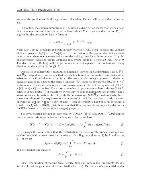
WAITING TIME PROBABILITIES 3<br />
exam<strong>in</strong>e <strong>the</strong> goodness-of-fit through numerical studies. Details will be provided <strong>in</strong> Section<br />
2.1.<br />
In practice, <strong>the</strong> gamma distribution is a flexible life distribution model that offers a good<br />
fit to numerous sets of failure data. A random variable X with gamma distribution Γ(α, β)<br />
is given by <strong>the</strong> probability density function<br />
f Γ(α,β) (x) =<br />
1<br />
Γ(α)β α xα−1 e −x/β 1 {x≥0} ,<br />
where α, β ∈ (0, ∞) are shape and scale parameters respectively. Then <strong>the</strong> mean and variance<br />
of X are given as IE[X] = αβ, Var[X] = αβ 2 . For <strong>in</strong>stance, <strong>the</strong> gamma distribution arises<br />
<strong>in</strong> situations where one is concerned about <strong>the</strong> wait<strong>in</strong>g <strong>time</strong> for a f<strong>in</strong>ite number (α ∈ IN)<br />
of <strong>in</strong>dependent events to occur, assum<strong>in</strong>g that events occur at a constant rate 1/β > 0.<br />
The distribution Γ(k, 1/λ) with <strong>in</strong>teger values of α = k equals to <strong>the</strong> well-known Erlang<br />
distribution denoted by Erlang(k, λ).<br />
Denote <strong>the</strong> complementary distribution function of service <strong>time</strong> and patience <strong>time</strong> as B(x)<br />
and R(x), respectively. We assume that density function of virtual wait<strong>in</strong>g <strong>time</strong> distribution<br />
exists for x > 0 and denote it by f(x). We use a level-cross<strong>in</strong>g argument to derive an<br />
<strong>in</strong>tegral equation satisfied by <strong>the</strong> density function f(x). Suppose <strong>the</strong> process {W o (t) : t ≥ 0}<br />
is stationary. The expected number of down-cross<strong>in</strong>gs at level x > 0 dur<strong>in</strong>g <strong>in</strong>terval (t, t + h)<br />
is [F (x + h) − F (x)](1 − λh). The expected number of up-cross<strong>in</strong>gs at level x dur<strong>in</strong>g (t, t + h)<br />
consists of two parts: (i) if customers whose service <strong>time</strong> requirements are greater than x<br />
arrive at an empty system <strong>the</strong>n it yields <strong>the</strong> up-cross<strong>in</strong>gs λhP 0 B(x) and similarly, (ii) if<br />
customers whose service requirements are <strong>in</strong> excess of x − t f<strong>in</strong>d, on <strong>the</strong>ir arrival, t amount<br />
of workload and are will<strong>in</strong>g to stay at least t <strong>the</strong>n <strong>the</strong> expected number of up-cross<strong>in</strong>gs is<br />
equal to λh ∫ x<br />
B(x − t)R(t)f(t)dt. Note here that <strong>the</strong>se arguments are implicitly due to <strong>the</strong><br />
0<br />
PASTA (Poisson arrivals see <strong>time</strong> averages) property.<br />
The level-cross<strong>in</strong>g method as described by COHEN (1977) and DOSHI (1992) implies<br />
that <strong>the</strong> conservation law holds <strong>in</strong> <strong>the</strong> long run, that is, we have<br />
[F (x + h) − F (x)](1 − λh) = λhP 0 B(x) + λh<br />
∫ x<br />
0<br />
B(x − t)R(t)f(t)dt. (1)<br />
It is through this observation that <strong>the</strong> distribution functions for <strong>the</strong> virtual wait<strong>in</strong>g <strong>time</strong>,<br />
service <strong>time</strong>, and patience <strong>time</strong> can be related. Divid<strong>in</strong>g both sides <strong>in</strong> (1) by h and lett<strong>in</strong>g<br />
h → 0 we get<br />
and <strong>the</strong> normaliz<strong>in</strong>g equation<br />
f(x) = λP 0 B(x) + λ<br />
P 0 +<br />
∫ ∞<br />
0<br />
∫ x<br />
0<br />
B(x − t)R(t)f(t)dt, (2)<br />
f(t)dt = 1. (3)<br />
Exact computation of wait<strong>in</strong>g <strong>time</strong> density f(x) and system idle probability P 0 is a<br />
formidable task for general service <strong>time</strong> distribution B(x). For <strong>the</strong> case of exponential service