Waiting time probabilities in the M/G/1 + M queue - Statistics ...

WAITING TIME PROBABILITIES 7
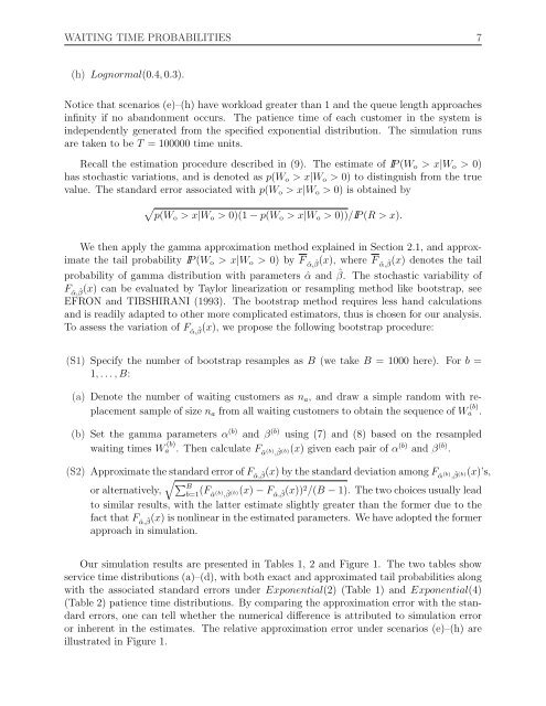
(h) Lognormal(0.4, 0.3).
Notice that scenarios (e)–(h) have workload greater than 1 and the queue length approaches
infinity if no abandonment occurs. The patience time of each customer in the system is
independently generated from the specified exponential distribution. The simulation runs
are taken to be T = 100000 time units.
Recall the estimation procedure described in (9). The estimate of IP (W o > x|W o > 0)
has stochastic variations, and is denoted as p(W o > x|W o > 0) to distinguish from the true
value. The standard error associated with p(W o > x|W o > 0) is obtained by
√
p(Wo > x|W o > 0)(1 − p(W o > x|W o > 0))/IP (R > x).
We then apply the gamma approximation method explained in Section 2.1, and approximate
the tail probability IP (W o > x|W o > 0) by F ˆα, ˆβ(x), where F ˆα, ˆβ(x) denotes the tail
probability of gamma distribution with parameters ˆα and ˆβ. The stochastic variability of
Fˆα, ˆβ(x) can be evaluated by Taylor linearization or resampling method like bootstrap, see
EFRON and TIBSHIRANI (1993). The bootstrap method requires less hand calculations
and is readily adapted to other more complicated estimators, thus is chosen for our analysis.
To assess the variation of Fˆα, ˆβ(x), we propose the following bootstrap procedure:
(S1) Specify the number of bootstrap resamples as B (we take B = 1000 here). For b =
1, . . . , B:
(a) Denote the number of waiting customers as n a , and draw a simple random with replacement
sample of size n a from all waiting customers to obtain the sequence of W (b)
a .
(b) Set the gamma parameters α (b) and β (b) using (7) and (8) based on the resampled
waiting times W (b)
a . Then calculate Fˆα (b) , ˆβ (b) (x) given each pair of α (b) and β (b) .
(S2) Approximate the standard error of Fˆα, ˆβ(x) by the standard deviation among Fˆα (b) , ˆβ (b) (x)’s,
or alternatively,
√ ∑B
b=1 (Fˆα (b) , ˆβ (b) (x) − Fˆα, ˆβ(x)) 2 /(B − 1). The two choices usually lead
to similar results, with the latter estimate slightly greater than the former due to the
fact that Fˆα, ˆβ(x) is nonlinear in the estimated parameters. We have adopted the former
approach in simulation.
Our simulation results are presented in Tables 1, 2 and Figure 1. The two tables show
service time distributions (a)–(d), with both exact and approximated tail probabilities along
with the associated standard errors under Exponential(2) (Table 1) and Exponential(4)
(Table 2) patience time distributions. By comparing the approximation error with the standard
errors, one can tell whether the numerical difference is attributed to simulation error
or inherent in the estimates. The relative approximation error under scenarios (e)–(h) are
illustrated in Figure 1.