Simulation of Synthetic Ground Motions for Specified Earthquake ...
Simulation of Synthetic Ground Motions for Specified Earthquake ...
Simulation of Synthetic Ground Motions for Specified Earthquake ...

You also want an ePaper? Increase the reach of your titles
YUMPU automatically turns print PDFs into web optimized ePapers that Google loves.
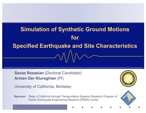
<strong>Simulation</strong> <strong>of</strong> <strong>Synthetic</strong> <strong>Ground</strong> <strong>Motions</strong><br />
<strong>for</strong><br />
<strong>Specified</strong> <strong>Earthquake</strong> and Site Characteristics<br />
Sanaz Rezaeian (Doctoral Candidate)<br />
Armen Der Kiureghian (PI)<br />
University <strong>of</strong> Cali<strong>for</strong>nia, Berkeley<br />
Sponsor: State <strong>of</strong> Cali<strong>for</strong>nia through Transportation Systems Research Program <strong>of</strong><br />
Pacific <strong>Earthquake</strong> Engineering Research (PEER) Center
Objective:<br />
Our Goal: <strong>Earthquake</strong> and site characteristics Suite <strong>of</strong> simulated design time-histories<br />
(F, M, R rup , V s30 ,…)<br />
Site<br />
Controlling Fault<br />
F: Faulting mechanism<br />
M: Moment magnitude<br />
…<br />
V s30 : Shear wave velocity <strong>of</strong> top 30m<br />
R rup : Closest distance to ruptured area<br />
What we have done so far:<br />
Developed a stochastic site-based model <strong>for</strong> far-field strong ground motions.<br />
Developed empirical predictive equations <strong>for</strong> the model parameters.<br />
Compared elastic response spectra (median and variability) to NGA relations.<br />
Ongoing activity and what we plan to accomplish by May 2010:<br />
Simulate orthogonal horizontal ground motion components.<br />
Extend the model to near-field ground motions.<br />
Scrutinize the simulated motions <strong>for</strong> inelastic structural responses.
<strong>Ground</strong> Motion Model:<br />
Acceleration<br />
Time modulating function<br />
Controls temporal nonstationarity<br />
Unit-variance process<br />
Controls spectral nonstationarity<br />
<br />
<br />
Time, sec<br />
<br />
<br />
Time, sec<br />
<br />
<br />
High-pass Filtering<br />
<br />
<br />
Time, sec
<strong>Ground</strong> Motion Model Parameters:<br />
Let:<br />
t 0<br />
t n<br />
t n<br />
: Arias intensity<br />
: Time at the middle <strong>of</strong> strong shaking<br />
: Effective duration<br />
t n
<strong>Ground</strong> Motion Model Parameters:<br />
Let:<br />
t 0<br />
t n<br />
t n<br />
: Arias intensity<br />
: Time at the middle <strong>of</strong> strong shaking<br />
: Effective duration<br />
t n<br />
If the model parameters are given, time-histories can be simulated.
Applications in Practice:<br />
<br />
Simulate a given accelerogram:<br />
…<br />
Acceleration, g<br />
0.15<br />
0<br />
Recorded<br />
-0.25<br />
0 40<br />
Time, sec<br />
Match<br />
statistical<br />
characteristics<br />
Representing:<br />
• Intensity<br />
• Frequency<br />
• Bandwidth<br />
Identify<br />
model parameters<br />
I a , t mid , D 5-95<br />
ω mid , ω’ , ζ<br />
model<br />
<strong>for</strong>mulation<br />
0.15<br />
0<br />
-0.25<br />
0.15<br />
0<br />
-0.25<br />
0.15<br />
0<br />
-0.25<br />
0<br />
…<br />
<strong>Simulation</strong>s<br />
40<br />
<br />
Simulate a suite <strong>of</strong> ground motions <strong>for</strong> a given design scenario:<br />
…<br />
0.1<br />
Given<br />
predictive<br />
<strong>Earthquake</strong>/Site characteristics<br />
equations<br />
(design scenario)<br />
F, M, R rup , V s30<br />
Generate<br />
several possible sets <strong>of</strong><br />
model parameters<br />
I a , t mid , D 5-95<br />
ω mid , ω’ , ζ<br />
model<br />
<strong>for</strong>mulation<br />
0<br />
-0.1<br />
0.1<br />
0<br />
-0.1<br />
0.1<br />
0<br />
-0.1<br />
0 5 10 15 20 25 30 35 40 45 50<br />
…<br />
<strong>Simulation</strong>s
Applications in Practice:<br />
<br />
Simulate a given accelerogram:<br />
…<br />
Acceleration, g<br />
0.15<br />
0<br />
Recorded<br />
-0.25<br />
0 40<br />
Time, sec<br />
Match<br />
statistical<br />
characteristics<br />
Representing:<br />
• Intensity<br />
• Frequency<br />
• Bandwidth<br />
Identify<br />
model parameters<br />
I a , t mid , D 5-95<br />
ω mid , ω’ , ζ<br />
Done <strong>for</strong> many records to get observational data<br />
<strong>for</strong> predictor and response variables<br />
model<br />
<strong>for</strong>mulation<br />
0.15<br />
0<br />
-0.25<br />
0.15<br />
0<br />
-0.25<br />
0.15<br />
0<br />
-0.25<br />
0<br />
…<br />
<strong>Simulation</strong>s<br />
40<br />
<br />
Simulate a suite <strong>of</strong> ground motions <strong>for</strong> a given design scenario:<br />
…<br />
0.1<br />
Given<br />
predictive<br />
<strong>Earthquake</strong>/Site characteristics<br />
equations<br />
(design scenario)<br />
Regression<br />
F, M, R rup , V s30<br />
Predictor variables<br />
Generate<br />
several possible sets <strong>of</strong><br />
model parameters<br />
I a , t mid , D 5-95<br />
ω mid , ω’ , ζ<br />
Response variables<br />
model<br />
<strong>for</strong>mulation<br />
0<br />
-0.1<br />
0.1<br />
0<br />
-0.1<br />
0.1<br />
0<br />
-0.1<br />
0 5 10 15 20 25 30 35 40 45 50<br />
…<br />
<strong>Simulation</strong>s
<strong>Ground</strong> Motion Database (far-field):<br />
<strong>Earthquake</strong> # <strong>of</strong> records <br />
1 Imperial Valley 2 <br />
2 Victoria, Mexico 2 <br />
3 Morgan hill 10 <br />
4 Landers 4 <br />
5 Big Bear 10 <br />
6 Kobe, Japan 4 <br />
7 Kocaeli, Turkey 4 <br />
8 Duzce, Turkey 2 <br />
9 Sitka, Alaska 2 <br />
10 Manjil, Iran 2 <br />
11 Hector Mine 16 <br />
12 Denali, Alaska 4 <br />
13 San Fernando 14 <br />
14 Tabas, Iran 2 <br />
15 Coalinga 2 <br />
16 N Palm Springs 12 <br />
17 Loma Prieta 28 <br />
18 Northridge 38 <br />
19 ChiChi, Taiwan 48 <br />
Total: 206 Accelerograms<br />
Strike-slip<br />
Reverse<br />
Moment Magnitude<br />
8.0<br />
7.5<br />
7.0 <br />
6.5 <br />
Shallow crustal earthquakes in<br />
tectonically active regions<br />
V s30 > 600 m/sec<br />
Two horizontal components<br />
6.0<br />
10 20 30 40 50 60 70 80 90 100<br />
R rup , km<br />
Strike-slip<br />
Reverse
Predictive Equations (Regression):<br />
<br />
Distributions assigned to the model parameters:<br />
Normalized Frequency (Total:206)<br />
0.4<br />
0.3<br />
0.2<br />
0.1<br />
0<br />
0.16<br />
0.12<br />
0.08<br />
0.04<br />
-7.5 -5.5 -3.5 -1.5 0<br />
0.08<br />
Normal<br />
0.06<br />
Beta 0.06<br />
Beta<br />
0.04<br />
0.02<br />
0<br />
4<br />
3<br />
2<br />
1<br />
5 10 15 20 25 30 35 40 45<br />
0.04<br />
0.02<br />
0<br />
0 5 10 15 20 25 30 35 40<br />
ln(I a , sec.g) D 5-95 , sec t mid , sec<br />
Gamma<br />
Two-Sided<br />
Exponential<br />
4<br />
3<br />
2<br />
1<br />
Beta<br />
Observed Data<br />
Fitted PDF<br />
0<br />
0 5 10 15 20 25<br />
ω mid /(2π), Hz<br />
0<br />
-2 -1.5 -1 -0.5 0 0.5<br />
ω'/(2π), Hz/sec<br />
0<br />
0 0.1 0.2 0.3 0.4 0.5 0.6 0.7 0.8<br />
ζ<br />
<br />
Regression model (<strong>for</strong> j th earthquake and k th record <strong>of</strong> that earthquake):<br />
Model parameter θ<br />
trans<strong>for</strong>med to the<br />
standard normal space<br />
Predicted mean<br />
conditioned on<br />
earthquake and site characteristics<br />
Independent<br />
Normally-distributed<br />
errors
Regression Results (Predictive Equations):<br />
Formulation:<br />
if<br />
if<br />
Maximum Likelihood Estimation:<br />
Standard deviation <strong>of</strong><br />
−1.844 −0.071 2.944 −1.356 −0.265 0.27 0.59 0.65<br />
−6.195 −0.703 6.792 0.219 −0.523 0.46 0.57 0.73<br />
−5.011 −0.345 4.638 0.348 −0.185 0.51 0.41 0.66<br />
2.253 −0.081 −1.810 −0.211 0.012 0.69 0.72 1.00<br />
−2.489 0.044 2.408 0.065 −0.081 0.13 0.95 0.96<br />
−0.258 −0.477 0.905 −0.289 0.316 0.68 0.76 1.02
Regression Results (Correlations):<br />
Trans<strong>for</strong>med model parameters:<br />
1 −0.36 0.01 −0.15 0.13 −0.01<br />
1 0.67 −0.13 −0.16 −0.20<br />
1 −0.28 −0.20 −0.22<br />
1 −0.20 0.28<br />
Symmetric<br />
1 −0.01<br />
1<br />
(given the earthquake and site characteristics)
Example 1 : Acceleration<br />
4 simulated motions and 1 real recording <strong>for</strong> the given design scenario:<br />
F = 1 (Reverse)<br />
M = 7.35<br />
R rup =14 km<br />
V S30 = 660 m/sec<br />
I a D 5-95<br />
sec.g sec<br />
RealizaVons <strong>of</strong> model parameters: <br />
t mid<br />
sec<br />
ω mid /(2π)<br />
Hz<br />
ω’/(2π)<br />
Hz/sec<br />
0.012 17.23 6.27 6.88 ‐0.01 0.14 <br />
0.145 12.30 6.78 5.90 0.12 0.26 <br />
0.055 14.22 7.22 4.48 ‐0.16 0.38 <br />
0.014 14.07 6.31 10.75 ‐0.24 0.26 <br />
0.036 14.87 8.32 4.36 ‐0.15 0.03 <br />
ζ<br />
Acceleration, g<br />
0.1<br />
0<br />
-0.1<br />
0 5 10 15 20 25 30 35<br />
0.2<br />
0<br />
-0.2<br />
0.2<br />
0<br />
0 5 10 15 20 25 30 35<br />
-0.2<br />
0 5 10 15 20 25 30 35<br />
0.1<br />
0<br />
-0.1<br />
0 5 10 15 20 25 30 35<br />
0.1<br />
0<br />
-0.1<br />
0 5 10 15 20 25 30 35<br />
Time, sec<br />
Simulated<br />
Recorded<br />
(1978 Tabas at Dayhook)<br />
Simulated<br />
Simulated<br />
Simulated
Example 1 : Velocity<br />
4 simulated motions and 1 real recording <strong>for</strong> the given design scenario:<br />
F = 1 (Reverse)<br />
M = 7.35<br />
R rup =14 km<br />
V S30 = 660 m/sec<br />
I a D 5-95<br />
sec.g sec<br />
RealizaVons <strong>of</strong> model parameters: <br />
t mid<br />
sec<br />
ω mid /(2π)<br />
Hz<br />
ω’/(2π)<br />
Hz/sec<br />
0.012 17.23 6.27 6.88 ‐0.01 0.14 <br />
0.145 12.30 6.78 5.90 0.12 0.26 <br />
0.055 14.22 7.22 4.48 ‐0.16 0.38 <br />
ζ<br />
Velocity, m/sec<br />
0.05<br />
0<br />
-0.05<br />
0 5 10 15 20 25 30 35<br />
0.2<br />
0<br />
-0.2<br />
0.2<br />
0<br />
0 5 10 15 20 25 30 35<br />
-0.2<br />
0 5 10 15 20 25 30 35<br />
0.1<br />
0<br />
Simulated<br />
Recorded<br />
Simulated<br />
Simulated<br />
0.014 14.07 6.31 10.75 ‐0.24 0.26 <br />
0.036 14.87 8.32 4.36 ‐0.15 0.03 <br />
-0.1<br />
0 5 10 15 20 25 30 35<br />
0.1<br />
0<br />
-0.1<br />
0 5 10 15 20 25 30 35<br />
Time, sec<br />
Simulated
Example 1 : Displacement<br />
4 simulated motions and 1 real recording <strong>for</strong> the given design scenario:<br />
F = 1 (Reverse)<br />
M = 7.35<br />
R rup =14 km<br />
V S30 = 660 m/sec<br />
I a D 5-95<br />
sec.g sec<br />
RealizaVons <strong>of</strong> model parameters: <br />
t mid<br />
sec<br />
ω mid /(2π)<br />
Hz<br />
ω’/(2π)<br />
Hz/sec<br />
0.012 17.23 6.27 6.88 ‐0.01 0.14 <br />
0.145 12.30 6.78 5.90 0.12 0.26 <br />
0.055 14.22 7.22 4.48 ‐0.16 0.38 <br />
ζ<br />
Displacement, m<br />
0.05<br />
0<br />
-0.05<br />
0 5 10 15 20 25 30 35<br />
0.1<br />
0<br />
-0.1<br />
0.1<br />
0<br />
-0.1<br />
0.05<br />
0<br />
Simulated<br />
Recorded<br />
0 5 10 15 20 25 30 35<br />
Simulated<br />
0 5 10 15 20 25 30 35<br />
Simulated<br />
0.014 14.07 6.31 10.75 ‐0.24 0.26 <br />
0.036 14.87 8.32 4.36 ‐0.15 0.03 <br />
-0.05<br />
0 5 10 15 20 25 30 35<br />
0.05<br />
0<br />
-0.05<br />
Simulated<br />
0 5 10 15 20 25 30 35<br />
Time, sec
Example 2 :<br />
If desired, a fixed value may be assigned to one or more <strong>of</strong> the model parameters:<br />
F = 1 (Reverse)<br />
M = 7.35<br />
R rup =14 km<br />
V S30 = 660 m/sec<br />
I a D 5-95<br />
sec.g sec<br />
RealizaVons <strong>of</strong> model parameters: <br />
t mid<br />
sec<br />
ω mid /(2π)<br />
Hz<br />
ω’/(2π)<br />
Hz/sec<br />
0.145 12.30 6.78 5.90 012 0.26 <br />
0.145 12.79 9.86 7.48 ‐0.52 0.13 <br />
0.145 22.11 16.24 8.05 ‐0.09 0.12 <br />
ζ<br />
Acceleration, g<br />
0.5<br />
0<br />
-0.5<br />
0 5 10 15 20 25 30 35 40<br />
0.5<br />
0<br />
-0.5<br />
0 5 10 15 20 25 30 35 40<br />
0.5<br />
0<br />
-0.5<br />
0 5 10 15 20 25 30 35 40<br />
0.5<br />
0<br />
Recorded<br />
Simulated<br />
Simulated<br />
Simulated<br />
0.145 8.14 5.31 7.34 ‐0.02 0.30 <br />
0.145 11.01 10.30 4.43 0.12 0.29 <br />
-0.5<br />
0 5 10 15 20 25 30 35 40<br />
0.5<br />
0<br />
-0.5<br />
0 5 10 15 20 25 30 35 40<br />
Time, sec<br />
Simulated
Example 3 : Response Spectrum (5% damped)<br />
2 horizontal components <strong>of</strong> a recorded motion (1994 Northridge at LA Wonderland Ave)<br />
Vs.<br />
50 simulated motions<br />
Corresponding to earthquake and site characteristics:<br />
F = 1 (Reverse)<br />
M = 6.69<br />
R rup = 20.3 km<br />
V S30 = 1223 m/sec<br />
10 1 5×10 0<br />
De<strong>for</strong>mation<br />
Response Spectrum, m<br />
10 0 5×10 0<br />
Recorded<br />
Simulated<br />
Pseudo-Acceleration<br />
Response Spectrum, g<br />
10 0<br />
10 -1<br />
10 -2<br />
10 -1<br />
10 -2<br />
10 -3<br />
10 -3<br />
10 -1 10 0<br />
Period, sec<br />
10 -4<br />
10 -1 10 0<br />
Period, sec
Comparison with NGA Models:<br />
10 0 M=6.0, R=20km<br />
10 -1<br />
Selected NGA Models:<br />
Campbell-Bozorgnia (z 2.5 = 1km)<br />
Abrahamson-Silva (z 1.0 = 34m)<br />
Chiou-Youngs (z 1.0 = 24m)<br />
Boore-Atkinson<br />
NGA Parameters:<br />
Rupture width = 20km<br />
Rupture depth = 1km<br />
<br />
10 -2<br />
5% Damped Pseudo-Acceleration Response Spectrum, g<br />
10 -3<br />
10 0 M=7.0, R=20km M=7.0, R=20km<br />
10 -1<br />
10 -2<br />
10 -3<br />
10 0 M=8.0, R=20km<br />
10 -1<br />
10 -2<br />
10 -3<br />
M=7.0, R=10km<br />
M=7.0, R=40km<br />
0.1 1.0 5.0 0.1 1.0<br />
Period, sec<br />
Period, sec<br />
5.0<br />
Avg NGA<br />
Median +1 logarithmic stdv.<br />
Median<br />
Median −1 logarithmic stdv.<br />
F = 0 (Strike-Slip)<br />
V s30 = 760 m/sec<br />
500 <strong>Simulation</strong>s<br />
Note:<br />
Models based on different subsets <strong>of</strong> NGA database.<br />
Observe:<br />
Except <strong>for</strong> M=6.0 (lower bound <strong>of</strong> database),<br />
deviations are much smaller than the variability<br />
present in the NGA prediction equations.<br />
<strong>Synthetic</strong>s are in close agreement with NGA.
Current & Future Developments:<br />
<br />
Simulating correlated orthogonal horizontal ground motion components.<br />
Component 1:<br />
Component 2:<br />
<strong>Motions</strong> in the database are rotated to the principal axes so that w 1 (τ) and w 2 (τ) are statistically independent.<br />
Model is fitted to the rotated database to estimate correlations: ρ α1, α2 and ρ λ1, λ2
Current & Future Developments:<br />
<br />
Simulating near-field ground motions.<br />
Separately model and superimpose:<br />
1) The directivity pulse<br />
Long period pulse in the velocity time-series <strong>of</strong> the fault-normal component.<br />
Develop prediction equations <strong>for</strong> characteristics <strong>of</strong> the pulse in terms <strong>of</strong> earthquake/site parameters.<br />
Collaboration with Jack Baker:<br />
Using wavelet analysis, directivity pulse extracted from a database <strong>of</strong> near-field motions,<br />
this database will be used to develop prediction equations.<br />
2) The fling step<br />
Permanent displacement may exist in the fault-parallel component.<br />
Incorporate the available seismological models (e.g., Somerville 1998, Abrahamson 2001).<br />
3) The residue motion<br />
The total motion minus the directivity pulse and the fling step.<br />
Model by a modified version <strong>of</strong> the far-field stochastic ground motion process.
Current & Future Developments:<br />
<br />
Scrutinize the simulated motions <strong>for</strong> inelastic structural responses.<br />
Compare inelastic response spectra (<strong>for</strong> given ductility ratios) <strong>of</strong> synthetic motions with real recordings and<br />
existing prediction equations (e.g., Bozorgnia et. al., 2010).<br />
Case Study:<br />
Compare inelastic response <strong>of</strong> a multi-degree-<strong>of</strong>-freedom structure to simulated and recorded motions.
Related Publications:<br />
Rezaeian, S. and A. Der Kiureghian,<br />
"A stochastic ground motion model with separable temporal and spectral nonstationarities,"<br />
<strong>Earthquake</strong> Engineering and Structural Dynamics, July 2008, Vol. 37, pp. 1565-1584.<br />
Rezaeian, S. and A. Der Kiureghian,<br />
"<strong>Simulation</strong> <strong>of</strong> synthetic ground motions <strong>for</strong> specified earthquake and site characteristics,"<br />
<strong>Earthquake</strong> Engineering and Structural Dynamics, 2009. Submitted.<br />
MATLAB s<strong>of</strong>tware to be made available<br />
Current abilities:<br />
Fitting the stochastic model to a target accelerogram.<br />
Simulating far-field strong motions on firm-ground <strong>for</strong> specified F, M, R rup , V s30 .<br />
Will be added by May 2010:<br />
Two component simulation.<br />
Near-field simulation.
Thank You
Features <strong>of</strong> target accelerogram<br />
<br />
<br />
Cumulative energy<br />
Cumulative energy<br />
<br />
<br />
<br />
Cumulative number <strong>of</strong> zero-level<br />
up crossings – a measure <strong>of</strong><br />
dominant frequency<br />
<br />
<br />
<br />
<br />
Cumulative number <strong>of</strong> zero level up crossings<br />
<br />
<br />
<br />
<br />
<br />
<br />
<br />
<br />
<br />
Cumulative number <strong>of</strong> positive minima and<br />
negative maxima – a measure <strong>of</strong> bandwidth<br />
Cumulative number <strong>of</strong> negative maxima<br />
and positive minima<br />
<br />
<br />
<br />
<br />
<br />
<br />
<br />
<br />
<br />
Time, sec
Response spectrum<br />
<br />
<br />
<br />
<br />
<br />
<br />
After high-pass filtering<br />
A(g)<br />
<br />
<br />
A(g)<br />
<br />
<br />
<br />
<br />
<br />
<br />
<br />
<br />
<br />
T (sec)<br />
Post-processing is needed <strong>for</strong> long<br />
-period range. A critically damped<br />
oscillator is used as a high-pass filter.<br />
<br />
<br />
<br />
Discretized<br />
white noise<br />
(input)<br />
Linear<br />
time-varying<br />
filter<br />
T (sec)<br />
Unit-variance process with<br />
spectral nonstationarity<br />
Time modulation<br />
corner frequency<br />
Fully non-stationarity<br />
process<br />
High-pass<br />
filter<br />
Simulated<br />
ground motion<br />
(output)
Northridge earthquake<br />
<br />
<br />
<br />
<br />
<br />
<br />
Recorded <br />
motion<br />
Acceleration, g<br />
<br />
<br />
<br />
<br />
<strong>Simulation</strong><br />
<br />
<br />
<br />
<br />
<br />
<br />
Time (sec)<br />
<strong>Simulation</strong>
Kobe earthquake<br />
Recorded <br />
motion<br />
Acceleration, g<br />
<strong>Simulation</strong><br />
<strong>Simulation</strong><br />
Time (sec)