A Guided Walk Down Wall Street: An Introduction to Econophysics

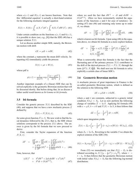
1048 Giovani L. Vasconcelos
where a(x, t) and B(x, t) are known functions. Note that
this ‘differential equation’ is actually a short-hand notation
for the following stochastic integral equation
X(t) = X(0)+
∫ t
0
a(X, t ′ )dt ′ +
∫ t
0
b(X, t ′ )dW (t ′ ). (41)
Under certain condition on the functions a(x, t) and b(x, t),
it is possible to show (see, e.g., [8]) that the SDE (40) has a
unique solution X(t).
Let us discuss another simple SDE, namely, the Brownian
motion with drift:
dX = µdt + σdW, (42)
where the constant µ represents the mean drift velocity. Integrating
(42) immediately yields the process
whose pdf is
X(t) = µt + W (t), (43)
p(x, t) = 1 { } (x − µt)
2
2πσ 2 t exp 2σ 2 . (44)
t
Another important example of a (linear) SDE that can be
solved explicitly is the geometric Brownian motion that will
be discussed shortly. But before doing that, let us discuss a
rather useful result known as Itô lemma or Itô formula.
3.5 Itô formula
Consider the generic process X(t) described by the SDE
(40), and suppose that we have a new stochastic process Z
defined by
Z(t) = F (X(t), t), (45)
for some given function F (x, t). We now wish to find the local
dynamics followed by the Z(t), that is, the SDE whose
solutions corresponds to the process Z(t) above. The answer
is given by the Itô formula that we now proceed to
derive.
First, consider the Taylor expansion of the function
F (X, t):
dF = ∂F ∂F
dt +
∂t ∂x dX + 1 ∂ 2 F
2 ∂x 2 (dX)2 +
+ 1 ∂ 2 F
2 ∂t 2 (dt)2 + 1 ∂ 2 F
dtdX + ... (46)
2 ∂t∂x
Note, however, that
(dX) 2 = b 2 dW 2 + 2ab dtdW + a 2 (dt) 2
= b 2 dt + O(dt 3/2 ), (47)
where we used the fact that dW 2 = dt and dtdW =
O(dt 3/2 ). (Here we have momentarily omitted the arguments
of the functions a and b for ease of notation.) Inserting
(47) into (46) and retaining only terms up to order
dt, we obtain
[ ∂F
dF =
∂t + 1 ]
2 b2 ∂2 F
∂x 2 dt + b ∂F dX, (48)
∂x
which is known as Itô formula. Upon using (40) in the equation
above, we obtain Itô formula in a more explicit fashion
[ ∂F
dF = + a(X, t)∂F
∂t ∂x + 1 ]
2 b2 (X, t) ∂2 F
∂x 2 dt
+ b(X, t) ∂F dW, (49)
∂x
What is noteworthy about this formula is the fact that the
fluctuating part of the primary process X(t) contributes to
the drift of the derived process Z(t) = F (t, X) through the
term 1 2 b2 (t, X) ∂2 F
∂x
. We shall next use Itô formula to solve
2
explicitly a certain class of linear SDE’s.
3.6 Geometric Brownian motion
A stochastic process of great importance in Finance is the
so-called geometric Brownian notion, which is defined as
the solution to the following SDE
dS = µSdt + σSdW, (50)
where µ and σ are constants, subjected to a generic initial
condition S(t 0 ) = S 0 . Let us now perform the following
change of variables Z = ln S. Applying Itô formula (49)
with a = µS, b = σS and F (S) = ln S, it then follows that
dZ =
(µ − 1 )
2 σ2 dt + σdW, (51)
which upon integration yields
Z(t) = Z 0 +
(µ − 1 )
2 σ2 (t−t 0 )+σ[W (t)−W (t 0 )], (52)
where Z 0 = ln S 0 . Reverting to the variable S we obtain the
explicit solution of the SDE (50):
S(t) = S 0 exp
{(µ − 1 )
}
2 σ2 (t − t 0 ) + σ[W (t) − W (t 0 )] .
(53)
From (52) we immediately see that Z(t) − Z 0 is distributed
according to N (( µ − 1 2 σ2) τ, σ √ τ ) , where τ =
t − t 0 . It then follows that the geometric Brownian motion
with initial value S(t 0 ) = S 0 has the following log-normal
distribution: