A Guided Walk Down Wall Street: An Introduction to Econophysics

1046 Giovani L. Vasconcelos
(22) and (23) then yields
[
lim E (Q n − t) 2] = 0.
n→∞
We have thus proven that Q n converges to t in the mean
square sense. This fact suggests that ∆W 2 can be thought
of as being of the order of ∆t, meaning that as ∆t → 0 the
quantity ∆W 2 “resembles more and more” the deterministic
quantity ∆t. In terms of differentials, we write
[dW ] 2 = dt. (24)
Alternatively, we could say that dW is of order √ dt:
dW = O( √ dt). (25)
(I remark parenthetically that the boundedness of the
quadratic variation of the Brownian motion should be
∑
contrasted with the fact that its total variation, A n =
n
i=0 |∆W i|, is unbounded, that is, A n → ∞ as n → ∞,
with probability 1; see [7].)
Another important property of the Brownian motion
W (t) is the fact that it is self-similar (or more exactly selfaffine)
in the following sense:
W (at) d = a 1/2 W (t), (26)
for all a > 0. Here d = means equality in the sense of probability
distribution, that is, the two processes W (at) and
a 1/2 W (t) have exactly the same finite-dimensional distributions
p(x 1 , t 1 ; ..., x n , t n ) for any choice of t i , i = 1, ..., n,
and n ≥ 1. Self-similarity means that any finite portion of
a Brownian motion path when properly rescaled is (statistically)
indistinguishable from the whole path. For example,
if we ‘zoom in’ in any given region (no matter how small)
of a Brownian motion path, by rescaling the time axis by a
factor of a and the vertical axis by a factor of √ a, we obtain
a curve similar (statistically speaking) to the original path.
An example of this is shown in Fig. 7. In the language of
fractals, we say that a trajectory of a Brownian motion is a
fractal curve with fractal dimension D = 2.
The self-similarity property implies that sample paths of
a Brownian motion are nowhere differentiable (technically,
with probability 1). A formal proof of this fact, although
not difficult, is beyond the scope of the present notes, so that
here we shall content ourselves with the following heuristic
argument. Suppose we try to compute the derivative of
W (t) in the usual sense, that is,
dW
dt
∆W
= lim
∆t→0 ∆t
= lim
∆t→0
W (t + ∆t) − W (t)
.
∆t
But since ∆W is of order √ ∆t, it then follows that
∆W
∆t
= O
so that dW/dt = ∞ as ∆t → 0.
( ) 1
√ , (27)
∆t
W(t)
W(t)
80
60
40
20
0
-20
-40
80
70
60
50
40
30
20
0 2000 4000 6000 8000 10000 12000 14000
t
5000 6000 7000 8000
t
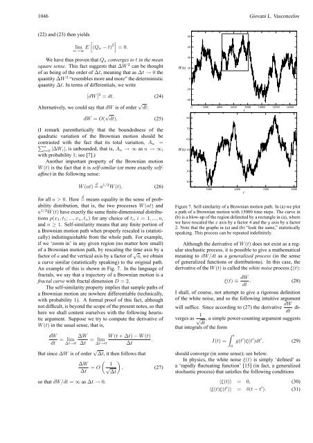
Figure 7. Self-similarity of a Brownian motion path. In (a) we plot
a path of a Brownian motion with 15000 time steps. The curve in
(b) is a blow-up of the region delimited by a rectangle in (a), where
we have rescaled the x axis by a factor 4 and the y axis by a factor
2. Note that the graphs in (a) and (b) “look the same,” statistically
speaking. This process can be repeated indefinitely.
Although the derivative of W (t) does not exist as a regular
stochastic process, it is possible to give a mathematical
meaning to dW/dt as a generalized process (in the sense
of generalized functions or distributions). In this case, the
derivative of the W (t) is called the white noise process ξ(t):
ξ(t) ≡ dW dt . (28)
I shall, of course, not attempt to give a rigorous definition
of the white noise, and so the following intuitive argument
will suffice. Since according to (27) the derivative dW diverges
as √ , a simple power-counting argument suggests
dt
1
dt
that integrals of the form
I(t) =
∫ t
0
g(t ′ )ξ(t ′ )dt ′ , (29)
should converge (in some sense); see below.
In physics, the white noise ξ(t) is simply ‘defined’ as
a ‘rapidly fluctuating function’ [15] (in fact, a generalized
stochastic process) that satisfies the following conditions
〈ξ(t)〉 = 0, (30)
〈ξ(t)ξ(t ′ )〉 = δ(t − t ′ ). (31)