DOI - UCSD VLSI CAD Laboratory

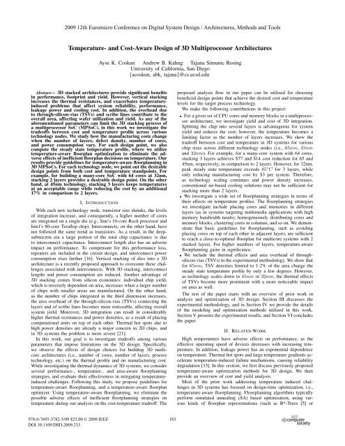
2009 12th Euromicro Conference on Digital System Design / Architectures, Methods and Tools
Temperature- and Cost-Aware Design of 3D Multiprocessor Architectures
Ayse K. Coskun Andrew B. Kahng Tajana Simunic Rosing
University of California, San Diego
{acoskun, abk, tajana}@cs.ucsd.edu
Abstract— 3D stacked architectures provide significant benefits
in performance, footprint and yield. However, vertical stacking
increases the thermal resistances, and exacerbates temperatureinduced
problems that affect system reliability, performance,
leakage power and cooling cost. In addition, the overhead due
to through-silicon-vias (TSVs) and scribe lines contribute to the
overall area, affecting wafer utilization and yield. As any of the
aforementioned parameters can limit the 3D stacking process of
a multiprocessor SoC (MPSoC), in this work we investigate the
tradeoffs between cost and temperature profile across various
technology nodes. We study how the manufacturing costs change
when the number of layers, defect density, number of cores,
and power consumption vary. For each design point, we also
compute the steady state temperature profile, where we utilize
temperature-aware floorplan optimization to eliminate the adverse
effects of inefficient floorplan decisions on temperature. Our
results provide guidelines for temperature-aware floorplanning in
3D MPSoCs. For each technology node, we point out the desirable
design points from both cost and temperature standpoints. For
example, for building a many-core SoC with 64 cores at 32nm,
stacking 2 layers provides a desirable design point. On the other
hand, at 45nm technology, stacking 3 layers keeps temperatures
at an acceptable range while reducing the cost by an additional
17% in comparison to 2 layers.
I. INTRODUCTION
With each new technology node, transistor size shrinks, the levels
of integration increase, and consequently, a higher number of cores
are integrated on a single die (e.g., Sun’s 16-core Rock processor and
Intel’s 80-core Teraflop chip). Interconnects, on the other hand, have
not followed the same trend as transistors. As a result, in the deepsubmicron
era a large portion of the total chip capacitance is due
to interconnect capacitance. Interconnect length also has an adverse
impact on performance. To compensate for this performance loss,
repeaters are included in the circuit design, and interconnect power
consumption rises further [16]. Vertical stacking of dies into a 3D
architecture is a recently proposed approach to overcome these challenges
associated with interconnects. With 3D stacking, interconnect
lengths and power consumption are reduced. Another advantage of
3D stacking comes from silicon economics: individual chip yield,
which is inversely dependent on area, increases when a larger number
of chips with smaller areas are manufactured. On the other hand,
as the number of chips integrated in the third dimension increases,
the area overhead of the through-silicon-vias (TSVs) connecting the
layers and of scribe lines becomes more noticeable, affecting overall
system yield. Moreover, 3D integration can result in considerably
higher thermal resistances and power densities, as a result of placing
computational units on top of each other. Thermal hot spots due to
high power densities are already a major concern in 2D chips, and
in 3D systems the problem is more severe [21].
In this work, our goal is to investigate tradeoffs among various
parameters that impose limitations on the 3D design. Specifically,
we observe the effects of design choices for building 3D multicore
architectures (i.e., number of cores, number of layers, process
technology, etc.) on the thermal profile and on manufacturing cost.
While investigating the thermal dynamics of 3D systems, we consider
several performance-, temperature-, and area-aware floorplanning
strategies, and evaluate their effectiveness in mitigating temperatureinduced
challenges. Following this study, we propose guidelines for
temperature-aware floorplanning, and a temperature-aware floorplan
optimizer. Using temperature-aware floorplanning, we eliminate the
possible adverse effects of inefficient floorplanning strategies on
temperature during our analysis on the cost-temperature tradeoff. The
proposed analysis flow in our paper can be utilized for choosing
beneficial design points that achieve the desired cost and temperature
levels for the target process technology.
We make the following contributions in this project:
• For a given set of CPU cores and memory blocks in a multiprocessor
architecture, we investigate yield and cost of 3D integration.
Splitting the chip into several layers is advantageous for system
yield and reduces the cost; however, the temperature becomes a
limiting factor as the number of layers increases. We show the
tradeoff between cost and temperature in 3D systems for various
chip sizes across different technology nodes (i.e., 65nm, 45nm
and 32nm). For example, for a many-core system with 64 cores,
stacking 3 layers achieves $77 and $14 cost reduction for 65 and
45nm, respectively, in comparison to 2 layers. However, for 32nm,
peak steady state temperature exceeds 85 o C for 3 layers, while
only reducing manufacturing cost by $3 per system. Therefore,
as technology scaling continues and power density increases,
conventional air-based cooling solutions may not be sufficient for
stacking more than 2 layers.
• We investigate a wide set of floorplanning strategies in terms of
their effects on temperature profiles. The floorplanning strategies
we investigate include placing cores and memories in different
layers (as in systems targeting multimedia applications with high
memory bandwidth needs), homogeneously distributing cores and
memory blocks, clustering cores in columns, and so on. We demonstrate
that basic guidelines for floorplanning, such as avoiding
placing cores on top of each other in adjacent layers, are sufficient
to reach a close-to-optimal floorplan for multicore systems with 2
stacked layers. For higher numbers of layers, temperature-aware
floorplanning gains in significance.
• We include the thermal effects and area overhead of throughsilicon-vias
(TSVs) in the experimental methodology. We show that
for 65nm, TSV densities limited to 1-2% of the area change the
steady state temperature profile by only a few degrees. However,
as technology scales down to 45nm or 32nm, the thermal effects
of TSVs become more prominent with a more noticeable impact
on area as well.
The rest of the paper starts with an overview of prior work in
analysis and optimization of 3D design. Section III discusses the
experimental methodology, and in Section IV we provide the details
of the modeling and optimization methods utilized in this work.
Section V presents the experimental results, and Section VI concludes
the paper.
II. RELATED WORK
High temperatures have adverse effects on performance, as the
effective operating speed of devices decreases with increasing temperature.
In addition, leakage power has an exponential dependence
on temperature. Thermal hot spots and large temperature gradients accelerate
temperature-induced failure mechanisms, causing reliability
degradation [15]. In this section, we first discuss previously proposed
temperature-aware optimization methods for 3D design. We then
provide an overview of cost and yield analysis.
Most of the prior work addressing temperature induced challenges
in 3D systems has focused on design-time optimization, i.e.,
temperature-aware floorplanning. Floorplanning algorithms typically
perform simulated annealing (SA) based optimization, using various
kinds of floorplan representations (such as B*-Trees [5] or
978-0-7695-3782-5/09 $25.00 © 2009 IEEE
DOI 10.1109/DSD.2009.233
183

Normalized Polish Expressions [23]). One of the SA-based tools
developed for temperature-aware floorplanning in 2D systems is
HotFloorplan [23].
Developing fast thermal models is crucial for thermally-aware
floorplanning, because millions of configurations are generated during
the SA process. Some of the typically used methods for thermal
modeling are numerical methods (such as finite element method
(FEM) [7]), compact resistive network [24], and simplified closedform
formula [6]. Among these FEM-based methods are the most
accurate and the most computationally costly, whereas closed-form
methods are the fastest but have lower accuracy.
In [8], Cong et al. propose a 3D temperature-aware floorplanning
algorithm. They introduce a new 3D floorplan representation called
combined-bucket-and-2D-array (CBA). The CBA based algorithm
has several kinds of perturbations (e.g., rotation, swapping of blocks,
interlayer swapping, etc.) which are used to generate new floorplans
in the SA engine. A compact resistive thermal model is integrated
with the 3D floorplanning algorithm to optimize for temperature. The
authors also develop a hybrid method integrating their algorithm with
a simple closed-form thermal model to get a desired tradeoff between
accuracy and computation cost.
Hung et al. [14] take the interconnect power into account in
their SA-based 3D temperature-aware floorplanning technique, in
contrast to most of the previous work in this area. Their results
show that excluding the interconnect power in floorplanning can
result in under-estimation of peak temperature. In Healy et al.’s
work on 3D floorplanning [11], a multi-objective floorplanner at the
microarchitecture level is presented. The floorplanner simultaneously
considers performance, temperature, area and interconnect length.
They use a thermal model that considers the thermal and leakage
inter-dependence for avoiding thermal runaway. Their solution consists
of an initial linear programming stage, followed by an SA-based
stochastic refinement stage.
Thermal vias, which establish thermal paths from the core of a chip
to the outer layers, have the potential to mitigate the thermal problems
in 3D systems. In [26], a fast thermal evaluator based on random
walk techniques and an efficient thermal via insertion algorithm are
proposed. The authors show that, inserting vias during floorplanning
results in lower temperatures than inserting vias as a post-process.
Cost and yield analyses of 3D systems have been discussed
previously, as in [18] and [10]. However, to the best of our knowledge,
a joint perspective on manufacturing cost and thermal behavior of
3D architectures has not been studied before. In this work, we
analyze the tradeoffs between temperature and cost with respect to
various design choices across several different technology nodes. For
thermally-aware floorplanning of MPSoCs, we compare several wellknown
strategies for laying out the cores and memory blocks against
floorplanning with a temperature-aware optimizer. In our analysis,
we use an optimization flow that minimizes the steady state peak
temperature on the die while reducing the wirelength and footprint
to achieve a fair evaluation of thermal behavior. Our experimental
framework is based on the characteristics of real-life components,
and it takes the TSV effects and leakage power into account.
III. METHODOLOGY
In this section we provide the details of our experimental methodology.
In many-core SoCs, the majority of the blocks on the die are
processor cores and on-chip memory (e.g., typically L2 caches). We
do not take the other blocks (I/O, crossbar, memory controller, etc)
into account in our experiments; however the guidelines we provide
in this study and the optimization flow are applicable when other
circuit blocks are included in the methodology as well.
A. Architecture and Power Consumption
We model a homogeneous multicore architecture, where all the
cores are identical. We model the cores based on the SPARC core
in Sun Microsystems’s UltraSPARC T2 [19], manufactured at 65nm
technology. The reason for this selection is that, as the number of
cores increase in multicore SoCs, the designers integrate simpler
cores as opposed to power-hungry aggressive architectures to achieve
the desired tradeoff between performance and power consumption
(e.g., Sun’s 8-core Niagara and 16-core Rock processors).
The peak power consumption of SPARC is close to its average
power value [17]. Thus, we use the average power value of 3.2W
(without leakage) at 1.2GHz and 1.2V [17], [19]. We compute
the leakage power of CPU cores based on structure areas and
temperature. For the 65nm process technology, a base leakage power
density of 0.5W/mm 2 at 383K is used [3]. We compute temperature
dependence using Eqn. (1), which is taken from the model introduced
in [12]. β is set at 0.017 for the 65nm technology [12].
P leak = P base · e β(Tcurrent−T 383)
(1)
P base =0.5 · Area (2)
To model cores manufactured at 45nm and 32nm technology
nodes, we use Dennard scaling supplemented by ITRS projections.
If k is the feature size scaling per technology generation, according
to Dennard scaling, for each generation we should observe that
frequency increases by a factor of k, while capacitance and supply
voltage decrease by a factor of k. ITRS projects that supply voltage
almost flatlines as scaling continues, scaling less than 10% per
generation. Using these guidelines, we set the dynamic average power
values of cores as in Table I, based on the equation P ∝ CV 2 f.
TABLE I. P OWER SCALING
Node Voltage Frequency Capacitance Power
65nm 1.2V 1.2GHz C 3.2W
45nm 1.1V 1.7GHz C/1.4 2.72W
32nm 1.0V 2.4GHz C/1.96 2.27W
Each L2 cache on the system is 1 MB (64 byte line-size, 4-
way associative, single bank), and we compute the area and power
consumption of caches using CACTI [25] for 65nm, 45nm and
32nm. At65nm the cache power consumption is 1.7W per each L2
including leakage, and this value also matches with the percentage
values in [17]. The power consumption of each cache block reduces
to 1.5W and 1.2W for 45nm and 32nm, respectively.
The area of the SPARC core in the 65nm Rock processor is
14mm 2 .For45nm and 32nm process technologies, we scale the
area of the core (i.e., area scaling is on the order of the square
of the feature size scaling). The area of the cores and caches for
each technology node are provided in Table II. As the area estimates
for cores and caches are almost equal, we assume the core and
cache areas for 65nm, 45nm, and32nm are 14mm 2 , 7mm 2 ,and
3.5mm 2 , respectively, for the sake of convenience in experiments.
This work assumes pre-designed IP blocks for cores and memories
are available for designing the MPSoC, so the area and dimensions
of the blocks are not varied across different simulations. We assume
a mesh network topology for the on-chip interconnects. Each core is
connected to an L2 cache, where the L2 caches might be private or
shared, depending on the area ratio of cores and memory blocks.
TABLE II. CORE AND CACHE AREA
Technology Core Area Cache Area
65nm 14mm 2 14.5mm 2
45nm 6.7mm 2 6.9mm 2
32nm 3.4mm 2 3.59mm 2
B. Thermal Simulation
HotSpot [24] provides temperature estimation of a microprocessor
at component or grid level by employing the principle of
electrical/thermal duality. The inputs to HotSpot are the floorplan,
package and die characteristics and the power consumption of each
component. Given these inputs, HotSpot provides the steady state
and/or the transient temperature response of the chip. HS3D has
184

TABLE III. PARAMETERS FOR THE THERMAL SIMULATOR
Parameter
Value
Die Thickness (one stack)
0.15mm
Convection Capacitance
140J/K
Convection Resistance
0.1K/W
Interlayer Material Thickness (3D)
0.02mm
Interlayer Material Resistivity (without TSVs) 0.25m K/W
extended HotSpot to 3D architectures [13] by adding a suite of
library functions. HS3D allows the simulation of multi-layer device
stacks, allowing the use of arbitrary grid resolution, and offering
speed increases of over 1000 X for large floorplans. HS3D has
been validated through comparisons to a commercial tool, Flotherm,
which showed an average temperature estimation error of 3 o C,and
a maximum deviation of 5 o C [14].
We utilize HotSpot Version 4.2 [24] (grid model), which includes
the HS3D features, and modify its settings to model the thermal
characteristics of the 3D architectures we are experimenting with.
Table III summarizes the HotSpot parameters. We assume that the
thermal package has cooling capabilities similar to typical packages
available in today’s processors. We calculate the die characteristics
based on the trends reported for 65nm process technology. Changing
the simulator parameters to model different chips and packages
affects the absolute temperature values in the simulation—e.g., thinner
dies are easier to cool and hence result in lower temperatures,
while higher convection resistance means that the thermal package’s
cooling capabilities are reduced and more hot spots can be observed.
However, the relative relationship among the results presented in this
work is expected to remain valid for similar multicore architectures.
HotSpot models the interface material between the silicon layers as
a homogeneous layer (characterized by thermal resistivity and specific
heat capacity values). To model the through-silicon-vias (TSV), we
assume a homogeneous via density on the die. The insertion of TSVs
is expected to change the thermal characteristics of the interface
material, thus, we compute the “combined” resistivity of the interface
material based on the TSV density. We compute the joint resistivity
for TSV density values of d TSV = {8, 16, 32, 64, 128, 256, 512}
per block; that is, a core or a memory block has d TSV vias
homogeneously distributed over its area. For example, in a 2-layered
3D system containing 16 SPARC cores and 16 L2 caches, there
is a total of 16 · d TSV vias on the die. Note that even if we had
wide-bandwidth buses connecting the layers, we would need a lot
less than 256 or 512 TSVs per block. We assume that the effect of
the TSV insertion to the heat capacity of the interface material is
negligible, which is a reasonable assumption, considering the TSV
area constitutes a very small percentage of the total material area.
Table IV shows the resistivity change as a function of the via
density for a 2-layered 3D system with 16 cores and 16 caches. In
our experiments, each via has a diameter of 10μm basedonthe
current TSV technology, and the spacing required around the TSVs
is also 10μm. The area values in the table refer to the total area of
vias, including the spacing.
TABLE IV. E FFECT OF VIAS ON THE INTERFACE RESISTIVITY
#Vias Via Area Area Resistivity
per Block (mm 2 ) Overhead (%) (mK/W )
0 0.00 0.00 0.25
8 0.12 0.05 0.248
16 0.23 0.10 0.247
32 0.46 0.20 0.245
64 0.92 0.40 0.24
128 1.84 0.79 0.23
256 3.69 1.57 0.21
512 7.37 3.09 0.19
IV. TEMPERATURE- AND COST-AWARE OPTIMIZATION
A. Yield and Cost Analysis of 3D Systems
Yield of a 3D system can be calculated by extending the negative
binomial distribution model as proposed in [18]. Eqns. (3) and (4)
show how to compute the yield for 3D systems with known-good-die
(KGD) bonding and for wafer-to-wafer (WTW) bonding, respectively.
In the equations, D is the defect density (typically ranging between
0.001/mm 2 and 0.0005/mm 2 [18]), A is the total chip area to be
split into n layers, α is the defect clustering ratio (set to 4 in all
experiments, as in [22]), A tsv is the area overhead of TSVs, and
P stack is the probability of having a successful stacking operation
for stacking known-good-dies. We set P stack to 0.99, representing
a highly reliable stacking process. Note that for wafer-to-wafer
bonding, per chip yield is raised to the n th power to compute the
3D yield. Wafer-to-wafer bonding typically incurs higher yield loss
as dies cannot be tested prior to bonding. In this work, we only focus
on die-level bonding.
Y system =[1+ D α ( A n + Atsv)]−α P stack n (KGD) (3)
Y system = {[1 + D α ( A n + Atsv)]−α } n (WTW) (4)
The number of chips that can be obtained per wafer is computed
using Eqn. (5) [9]. In the equation, R is the radius of the wafer and
A c is the chip area, including the area overhead of TSVs and scribe
lines. The scribe line overhead of each chip is L s(2 √ A/n + L s),
where L s is the scribe line width (set at 100μm in out experiments).
Note that for a 3D system with n layers, the number of systems
manufactured out of a wafer is U 3d = U/n. Weassumeastandard
300mm wafer size in all of the experiments.
U = πR − 2π √ R + π (5)
A c Ac
Fig. 1. Utilization, Yield and Cost ($). Utilization is normalized with respect
to the 2D chip of equivalent total area.
Once we know the yield and wafer utilization, we compute the
cost per 3D system using Eqn. (6), where C wafer is the cost of the
wafer in dollars. We set C wafer = $3000 in our experiments.
C wafer
C =
(6)
U 3d · Y system
The wafer utilization, yield and cost of systems with a total area
ranging from 100mm 2 to 400mm 2 and with various numbers of
stacked layers are provided in Figure 1. We observe that 3D stacking
improves yield and reduces cost up to a certain number of stacked
layers (n). As n is increased further, yield saturates and then drops
mainly due to the drop in the probability of successfully stacking n
layers (i.e., the Pstack n parameter). These results for yield and cost
motivate computing the desired cost-efficiency points for a given
design before deciding on the number of layers and size of a 3D
architecture. In addition, we see that partitioning chips with area
100mm 2 and below does not bring benefits in manufacturing cost.
185

1 2
3 4
Layer-2
5 6
7 8
Layer-1
NPEs of 2D Layers NPE of 3D System
V
V
H H
H H
1 3 2 4
L L L L
V
H H
1 5 3 7 2 6 8 4
5 7 6 8
Fig. 2. Example NPE Representation.
(1) (2) (3)
LEGEND
Heat Sink
core Spreader
Layer-2 Layer-2 Layer-2 memory
Interface Material
Layer-2
Interface Material
Layer-1 Layer-1 Layer-1
Layer-1
Fig. 3. Known-Good Floorplans for the Example Systems.
B. Temperature-Aware Floorplan Optimization
For a given set of blocks and a number of layers in the 3D
system, we use HotFloorplan [23] for temperature-aware floorplan
optimization. Using a simulated annealing engine, the HotFloorplan
tool can move and rotate blocks, and vary their aspect ratios, while
minimizing a pre-defined cost function.
A commonly used form of cost function in the literature (e.g., [11])
is shown in Eqn. (7), where a, b and c are constants, W is the
wirelength, T is the peak temperature and A is the area. Minimizing
f minimizes the communication cost and power consumption associated
with interconnects, and also minimizes the chip area while
reducing the peak temperature as much as possible.
f = a · W + b · T + c · A (7)
The wirelength component in Eqn. (7) only considers the wires
connecting the cores and their L2 caches in this work. As we
are integrating pre-designed core and cache blocks, the wirelengths
within each block are the same across all simulations. To compute
the wirelength, we calculate the Manhattan distance between the
center of a core and the center of its L2 cache, and weigh this value
based on the wire density between the two units. However, as we are
experimenting with a homogeneous set of cores and caches, the wire
density is the same across any two components, and is set to 1.
We use fixed aspect ratios of cores and memory blocks as in a reallife
many-core SoC design scenario, where IP-cores and memories
with pre-determined dimensions are integrated. This simplification
reduces the simulation time for the floorplanner. Thus, instead of
a two-phase optimization flow of partitioning and then floorplanning
(e.g., [14], [1]), we are able to perform a one-shot optimization, where
the blocks can be moved across layers in the annealing process.
HotFloorplan represents floorplans with Normalized Polish Expressions
(NPEs), which contain a set of units (i.e., blocks in
the floorplan) and operators (i.e., relative arrangement of blocks).
The design space is explored by the simulated annealer using the
following operators: (1) swap adjacent blocks, (2) change relative
arrangement of blocks, and (3) swap adjacent operator and operand.
For 3D optimization, we extend the algorithm in HotFloorplan with
the following operators defined in [14]: (1) Move a block from
one layer to another (interlayer move), and (2) Swap two blocks
between 2 layers (interlayer swap). As we utilize fixed-size cores
and caches in this paper, the interlayer move can be considered as an
interlayer swap between a core or memory and a “blank” grid cell in
the floorplan. These moves still maintain the NPEs, and satisfy the
balloting property (which verifies the resulting NPE as valid) [1].
NPE representations for an example 3D system are provided in
Figure 2. While the letters V and H demonstrate horizontal and
vertical cuts, L represents different stacks in the system.
C. Sensitivity Analysis of the Optimizer
For verification of the optimizer, we compare the results obtained
by the optimizer to known-best results for several experiments. We
use smaller sample 3D systems to reduce the simulation time in
the verification process. All samples are 2-layered 3D systems, and
they have the following number of cores and caches: (1) 4 cores
and 4 memory blocks, (2) 6 cores and 2 memory blocks, and (3) 2
cores and 6 memory blocks. The known-best results are computed
by performing exhaustive search for a fixed footprint area. For each
of the three cases, the optimizer result is the same as the result of
the exhaustive search. The solutions for the example set are shown
in Figure 3.
We also run a set of experiments for larger MPSoCs to verify the
SA-based optimizer: an 8-core MPSoC and an 18-core MPSoC, both
with 4 layers and with equal number of cores and L2 caches. In all of
our experiments, we observe that optimal results avoid overlapping
cores on adjacent layers on top of each other. Therefore, we only
simulate floorplans that do not overlap cores in adjacent layers. When
no cores can overlap, for a 4-layered system without any “blank”
cells (i.e., the core and memory blocks fully utilize the available
area) and with equal areas of caches and cores, there are 3 n different
floorplans. The reason for the 3 n is that, considering a vertical column
of blocks (i.e., blocks at the same grid location on each layer), there
are 3 possible options of cache/core ordering, without violating the
no-overlap restriction. These three possible orderings (from top layer
to bottom layer) are: (1) C-M-C-M, (2) C-M-M-C, and (3) M-C-M-C,
where M and C represent a memory block and a core, respectively.
For the 8-core MPSoC, we simulate all possible floorplans that
abide by the restriction of not overlapping cores and that minimize
the wirelength. This search constitutes a solution space of 3 4 =81
different designs, where all designs have 4 components on each layer
(2x2 grid). For the 18-core MPSoC, similarly we have 9 components
on each layer in a 3x3 grid, and we simulate 1000 randomly selected
floorplans that maintain the same restriction for overlapping cores
(among a solution space of 3 9 floorplans). In both experiments, we
select the floorplan with the lowest steady state peak temperature
at the end. The optimizer result is the same as the best floorplan
obtained in the 8-core experiment. In the 18-core case, the optimizer
results in 1.7 o C lower temperature than the best random solution.
As a second step in the verification process, we perform a study
on how the coefficients in the cost function affect the results of the
optimizer. This step is also helpful in the selection of coefficients.
Note that the area (A) in Eqn. (7) is in hundreds of millimeters,
temperature (T ) in several hundred Kelvin degrees, and wirelength
(W ) is in tens of millimeters. The range of constants used in this
experiment takes the typical values of A, T and W into account.
Fig. 4.
Effect of Cost Function Parameters on Temperature.
Figure 4 demonstrates how the peak steady state temperature
achieved by the floorplan changes when the wirelength coefficient
(a) varies (other constants fixed), and when area coefficient (c) varies
(again other constants fixed). Note that for a 2-layered system with
an equal number of cores and memories, the optimizer minimizes the
wirelength by placing a core and its associated L2 on top of each
other. Therefore, changing the coefficient of the wirelength does not
change the solution as placing a core and its L2 on top of each
other provides the smallest total wire distance. To create a more
interesting case for wirelength minimization, we use a 2-layered 3D
system with core-to-memory ratio (CMR) of 0.5. For investigating the
186

Cost per System ($)
1000
100
10
1
8 16 32 64 8 16 32 64 128 8 16 32 64 128 256
65nm 45nm 32nm
Number of Cores
Fig. 5. Cost Change Across Technology Nodes.
n=1
n=2
n=3
n=4
n=5
n=6
n=10
System ($)
Cost per
140
120
100
80
60
40
20
0
65nm
1 2 3 4 5 6 10
n (# of stacked layers)
D
(1/mm^2)
0.001
0.002002
0.003
0.004
System ($)
Cost per
45
40
35
30
25
20
15
10
5
0
1 2 3 4 5 6 10
n (# of stacked layers)
16 cores
32 cores
64 cores
Fig. 6.
Effect of Defect Density on System Cost.
Fig. 7.
Change in Cost with respect to Number of Cores and Layers.
effect of the area coefficient, we use fewer memory blocks than cores
(CMR =2), to see a more significant effect on peak temperature.
In HotFloorplan, the interconnect delay is computed using a first
order model based on [2] and [20]. While more accurate delay models
exist in literature, such as [4], in our experiments the first order model
is sufficient. This is due to the fact that the floorplanner tends to place
cores and their memories on adjacent layers and as close as possible
to each other to reduce the wirelength (recall that the distance for
vertical wires are much shorter than horizontal ones in general). Thus,
increasing the accuracy of the wire delay model does not introduce
noticeable differences in our experiments.
Based on the results presented, we selected the coefficients as a =
0.4, b =1,andc =4. Similar principles stated above can be utilized
for selecting the coefficients for different 3D systems.
V. EXPERIMENTAL RESULTS
In this section, we discuss the results of our analysis on the
manufacturing cost and thermal behavior of 3D systems. First, we
demonstrate how the cost changes depending on defect density,
number of cores and number of layers for 65nm, 45nm and 32nm
technology nodes. We then evaluate various floorplanning strategies,
and compare the results against our temperature-aware floorplanner.
Finally, the section concludes by pointing out the tradeoffs between
cost and temperature for a wide range of design choices, and
providing guidelines for low-cost reliable 3D system design.
A. Design Space Exploration for 3D System Cost
We summarize the variation of cost across the process technologies
65nm, 45nm and 32nm in Figure 5. In this experiment, the defect
density is set at 0.001/mm 2 , and the core to memory ratio (CMR) is
1 (i.e., each core has a private cache). We compute the cost up to 256
cores for each node, but omit the results in the figure for the cases
where per-system cost exceeds $1000 (note that the y-axis is on a
logarithmic scale). For building MPSoCs with a high number of cores,
3D integration becomes critical for achieving plausible system cost.
Technology scaling provides a dramatic reduction in cost, assuming
that the increase in defect density is limited.
Defect density is expected to increase as the circuit dimensions
shrink. Thus, to evaluate how the cost is affected by the change in
defect density (D), in Figure 6 we show the cost per system in dollars
(y-axis), and the x-axis displays the number of stacked layers in the
system (keeping the total area to be split the same). There are 16 cores
and 16 memory blocks in the 3D architecture (i.e., CMR =1), and
the technology node is 65nm. In all of the experiments in this section,
the TSV count is set to a fixed number of 128 per chip. Especially if
the defect density is high, 3D integration brings significant benefits.
For example, for a defect density of 0.003/mm 2 , splitting the 2D
system into 2 layers reduces the cost by 46%, and splitting into 4
layers achieves a cost reduction of 61%. In the rest of the experiments
we use a defect density of 0.001/mm 2 , representing mature process
technologies.
In Figure 7, we demonstrate the change of cost with respect to
the number of layers and number of cores for 32nm technology.
The CMR is again 1 in this experiment. For the 16-core system,
the minimum cost is achieved for 4 layers, and for the 32-core
case integrating 6 layers provides the minimum system cost. As
the number of cores, or in other words, total area increases, we
may not reach the minimum point for the cost curve by integrating
a reasonable number of layers—e.g., for 64 cores, integrating 10
layers seems to give the lowest cost in the figure, which may result
in unacceptable thermal profiles. Therefore, especially for manycore
systems, an optimization flow that considers both the cost and
temperature behavior is needed, as increasing the number of stacked
layers introduces conflicting trends in thermal behavior and yield.
We observe that TSVs do not introduce noticeable impact on yield
and cost, as long as the ratio of TSV area to chip area is kept lower
than only a few percents. For 45nm technology, the cost difference
between a fixed TSV count of 128 and a fixed TSV percentage of
1% is shown in Figure 8. n demonstrates the number of layers as
before. For example, when we compare keeping the TSV density
at 1% of the chip area against using a fixed number (i.e., 128) of
TSVs per chip, up to 64 cores, the cost difference between the two
cases is below $1. As the number of cores and overall area increase,
accommodating TSVs occupying 1% of the chip area translates to
integrating thousands of TSVs. Thus, for many-core systems, TSV
overhead becomes a limiting factor for 3D design.
B. Thermal Evaluation of 3D Systems
In this section, we evaluate the thermal behavior for various design
choices in 3D systems. To understand the effects of temperature-
187

Temperature (C)
74
72
70
68
66
64
62
exp1
exp2
exp3
exp4ab
exp4ba
exp5ab
exp5ba
exp6_1
exp6_2
exp1b
exp4ab_rot
Fig. 10.
MAX MAX_TSV512
Peak Steady State Temperature Comparison.
Fig. 8. TSV cost difference between using a fixed count and a fixed
percentage (45nm).
exp1 exp2 exp3 exp4ab exp4ba
Layer-2 Layer-2 Layer-2 Layer-2 Layer-2
Layer-1 Layer-1 Layer-1 Layer-1 Layer-1
Gradient (C)
12
10
8
6
4
2
0
exp1
exp2
exp3
exp4ab
MAX GRAD
MAX LAYER GRAD
exp4ba
exp5ab
exp5ba
exp6_1
exp6_2
exp1b
exp4ab_rot
MAX GRAD_TSV512
MAX LAYER GRAD_TSV512
Fig. 11. Comparison of Gradients.
exp5ab
exp5ba
exp6_1
exp6_2
Layer-2
Layer-1
exp1b
Layer-2
Layer-1
Layer-2
Layer-1
exp4ab_rot
Fig. 9.
Layer-2
Layer-1
Layer-2
Layer-1
Floorplans.
Layer-2
Layer-1
LEGEND
core
memory
Heat Sink
Spreader
Interface Material
Layer-2
Interface Material
Layer-1
aware optimization and also to ensure that our results are not
biased by floorplanning decisions, we first analyze the effects of 3D
floorplanning on temperature. All the simulation results shown in this
section are for the 65nm technology.
1) Comparing Floorplanning Strategies: To investigate how floorplanning
affects the thermal profile, we experiment with a 16-core
system with the architectural characteristics described in Section III.
Each core has an L2 cache, so we have a total of 16 cores and 16
memory blocks. The various floorplans we use in our simulations are
summarized in Figure 9.
Figure 10 demonstrates the peak steady state temperature achieved
by each floorplan. MAX shows the results without considering the
TSV modeling, and MAX TSV512 represents the results that take into
account the TSV effect on temperature, with TSV density of 512 per
block. Even though 512 vias per block is a significantly large number,
there is only a slight reduction in the steady state peak temperature
(i.e., less than 1 o C). For this reason, we do not plot the thermal results
with all the TSV densities that we experiment with. For the rest of
the results, we use a TSV density of 512 per block, representing a
best-case scenario for temperature.
For the 2-layer 3D system, exp3, which places all the cores on
the layer adjacent to the heat spreader and all memories in the lower
layer, has the lowest temperature. exp4ab also achieves significant
reduction of peak temperature in comparison to other strategies, and
the wirelength is the same. Note that in both floorplans the core can be
overlapped in adjacent layers with its L2 cache. All the floorplans that
increase the peak temperature (e.g., exp1b) have overlapping cores in
adjacent layers.
In addition to thermal hot spots, large spatial gradients (i.e.,
temperature differences among different locations on the chip) cause
challenges in performance, reliability and cooling efficiency, so
gradients with lower magnitudes are preferable. In Figure 11, we
compare the maximum spatial gradient among the blocks at steady
state. MAX GRAD and MAX LAYER GRAD represent the gradient
across all blocks (considering all layers) and the maximum intralayer
gradient (the gradients across layers are not taken into account),
respectively. The traces with the TSV suffix are from the simulations
including the TSV modeling. We see that exp3 also outperforms the
other strategies for reducing the gradients on the die.
2) The Effect of the Ratio of Core and Memory Area: In Section V-
B.1, all the 3D systems have an equal number and area of cores
and memories. Next, we look into how the change in CMR affects
the thermal behavior. For this experiment, we simulate various CMR
values, but we only show the results for CMR =2and CMR =0.5
as the trends for other ratios are similar.
In Figures 12 and 13, we compare the peak temperature and largest
gradient for the floorplans generated by the optimizer for core-tomemory
area ratios of 2, 0.5, and 1 (baseline). While the peak
temperature is positively correlated with the number of cores, the
temperature gradients increase when the CMR is different than 1.
Thus, separating the core and memory layers as much as possible is
a good solution for reducing the gradients as well.
For 2-layered 3D architectures, following basic guidelines such
as avoiding a vertical overlap of cores (or in general, power-hungry
units), and placing the units with higher power consumption closer to
the heat sink achieve very similar results to the known-best solutions.
These two principles prove to be more significant than avoiding the
placement of cores in adjacent locations horizontally in a multicore
3D system. This general rule-of-thumb holds for any CMR value.
When CMR < 1, separating the cores on the same layer as much
as possible is also necessary for achieving better thermal profiles.
3) The Effect of the Number of Stacks on Temperature: The
purpose of the next experiment is to observe the effect of increasing
188

Fig. 12.
ady State
ature (C)
Peak Stea
Tempera
72
70
68
66
64
62
60
58
CMR-2 CMR-0.5 BASE (CMR-1)
Comparison of Peak Temperature - Core to Memory Area Ratio.
dy State
ture (C)
Peak Stead
Temperat
90
85
80
75
70
65
60
55
50
exp1 exp3 exp4ab
2-layer
4-layer
Maximum m Spatial
Gradie ent (C)
Fig. 13.
5
4
3
2
1
0
CMR-2 CMR-0.5 BASE (CMR-1)
MAX GRAD
MAX LAYER GRAD
Comparison of Gradients - Core to Memory Area Ratio.
the number of stacks on peak steady state temperature and the
temperature gradients. We compare a 2-layered 3D stack architecture
against a 4-layered architecture using the same number of cores and
memories to achieve a fair comparison. In other words, the total
power consumption of the cores and memories are the same in the
2- and 4-layered systems in Figure 14.
Figure 14 compares the peak steady state temperature of the 2-
and 4-layered systems for several floorplanning strategies shown
in Figure 9. In the 4-layered systems, the floorplanning patterns
for upper and lower layers are repeated; e.g., for exp3, wehavea
core layer, a memory layer, again a core layer and a memory layer
(ordered from top layer to bottom). In Figure 15, we demonstrate
the spatial gradients on the systems. For the 4-layered systems, we
observe a significant increase in the gradients across the chip (i.e.,
MAX GRAD). This is because the temperature difference between
the layers close to and far away from the heat sink increases with
higher number of layers in the 3D stack.
In the example shown in Figures 14 and 15, for the 4-layered
stack the footprint reduces by 44% and the system cost decreases by
close to 40% in comparison to using a 2-layered stack (i.e., for a
system that contains the same number of cores and caches). On the
other hand, we see a noticeable increase in temperature. Hence, for
multicore systems, temperature-aware floorplanning becomes crucial
for systems with a higher number of stacked layers.
4) Optimizer Results: We have seen in the last section that for
3D systems with a high number of vertical layers, temperature-aware
optimization is a requirement for reliable design. Figure 16 compares
the optimizer results for a 4-layered 3D system (containing 16 cores
and 16 L2 caches) to the best performing custom strategies investigated
earlier. All the floorplans investigated in Figure 16 have the
same footprint. This is an expected result as we keep the dimensions
of the memory blocks and cores fixed during optimization, and the
optimization flow (which minimizes the total area as well) results in
the same footprint area as the hand-drawn methods. We show the
resulting floorplan of the optimizer in Figure 17, where the darker
blocks are cores, and Layer-4 is the layer closest to heat sink. Note
that there are other floorplans that have the same lowest steady state
peak temperature.
For 4-layered systems, the optimizer achieves an additional 5%
of peak temperature reduction in comparison to the best performing
hand-drawn floorplan. The benefits of optimization are more substantial
for a higher number of stacked layers. As the number of
layers increases, reducing the peak steady state temperature through
floorplan optimization becomes more critical for reducing the adverse
effects of high temperatures at runtime—this is because the dynamic
Gradient (C)
Maximum Spatial
Fig. 15.
Fig. 14.
14
12
10
8
6
4
2
0
Comparison of 2- and 4-Layered Systems.
exp1 exp3 exp4ab
2-layer, MAX_GRAD
4-layer, MAX_GRAD
2-layer, MAX_LAYER_GRAD
4-layer, MAX_LAYER_GRAD
Comparison of Spatial Gradients in 2- and 4-Layered Systems.
temperature range at runtime is highly dependent on the steady state
behavior of the system.
Even though we do not explicitly model the interconnect power
consumption, the accuracy impact of this is expected to be minimal.
This is because all of the floorplanning strategies in this example
(i.e., both custom designed strategies and the optimizer results) place
cores and their associated L2 caches on adjacent layers, and overlap
them to minimize the total amount of interconnects. As noted earlier,
the TSV length is dramatically less than the horizontal interconnects,
as the thickness of the interlayer material is 0.02mm.
C. Investigating the Temperature-Cost Trade-Off
Next we discuss the design tradeoff between cost and temperature
profiles for 65nm, 45nm and 32nm technology nodes. Figure 18
demonstrates the cost per system in dollars and the peak steady state
temperature for the system with 64 cores and 64 L2 caches. All the
thermal results in this section utilize the temperature-aware floorplan
optimizer discussed previously.
The common trend in the figure is that, going from a single layer
chip to 2 layers, both the cost and temperature decrease considerably.
The decrease in temperature is a result of the vertical heat transfer
from the cores to their memories, which have considerably lower
temperatures. Thus, in addition to dissipating heat through the heat
spreader and sink, the cores transfer part of their heat to their caches
and end up with several degrees of cooler temperature. However, if
3D stacking overlaps cores in the adjacent layers (e.g., in the case
where the number of cores is more than that of caches), steady state
temperature is expected to increase.
Also, note that the cost per system drops significantly with each
process technology. This sharp drop results from the simultaneous
increase in yield and wafer utilization when the same chip is
manufactured at a smaller technology node.
Another important observation regarding Figure 18 is that, for
65nm and 45nm, it is possible to reduce the per-system cost
significantly by partitioning the system into 3 layers; i.e, $77 and
$14 reduction for 65nm and 45nm, respectively, in comparison
to building the same system with 2 layers. However, for 32nm,
peak steady state temperature exceeds 85 o C for n =3, while only
reducing the cost by approximately $3. Therefore, as technology
scaling continues and power density increases, it may not be feasible
to stack more than 2 layers for systems with conventional cooling.
189

Peak Tem mperature (C)
88
86
84
82
80
78
76
74
72
70
exp1 exp3 exp4ab OPT
20
18
16
14
12
10
8
6
4
2
0
dient (C)
Grad
Fig. 16.
Peak (Left-Axis) MAX_GRAD (Right-Axis) MAX_LAYER_GRAD (Right-Axis)
Peak Temperature and Gradients - Comparison to Optimizer Results.
Fig. 18. Cost and Temperature for a 64-Core MPSoC: bar graphs show cost
on the left y-axis, and line graphs show peak temperature on the right axis.
Fig. 17.
Optimizer Result for the 4-Layered 16 Core MPSoC.
Also, the heat density increases rapidly for a higher number of
cores. 3D integration for many-core systems in 45nm and below will
require more efficient cooling infrastructures, such as liquid cooling.
VI. CONCLUSION
3D integration is a promising solution for shortening wirelength,
and for reducing the power consumption and delay of interconnects
on SoCs. In addition, partitioning large chips into several layers
increases yield and reduces the cost. One critical issue in 3D design
is that vertical stacking exacerbates the challenges associated with
high temperatures.
In this work, we presented an analysis infrastructure, evaluating
both manufacturing cost and temperature profile of 3D stack architectures
across current and future technology nodes. We utilized a
temperature-aware floorplanner to eliminate any adverse effects of
inefficient placement while evaluating the thermal profile. As a result
of our floorplanning study, we have provided guidelines for thermalaware
floorplanning in 3D architectures. For 3D systems with more
than 2 layers, we showed that using an optimizer provides significant
advantages for reducing peak temperature.
Using our framework, we presented experimental results for a
wide range of assumptions on process technology characteristics and
design choices. For example, for a 45nm many-core SoC with 64
cores, stacking 3 layers cuts the manufacturing cost in half compared
to a single-layer chip, while still maintaining a peak temperature
below 85 o C. When the same system is manufactured at 32nm,
stacking 2 layers and 3 layers reduces the cost by 25% and 32%,
respectively, compared to the 2D chip. However, at 32nm, the steady
state peak temperature for 3 layers reaches 87 o C, due to the increase
in the power density. Such results emphasize that using a joint
evaluation of cost and temperature is critical to achieve cost-efficient
and reliable 3D design.
ACKNOWLEDGEMENTS
The authors would like to thank Prof. Yusuf Leblebici at EFPL for his valuable
feedback. This work has been funded in part by Sun Microsystems, UC
MICRO, Center for Networked Systems (CNS) at UCSD, MARCO/DARPA
Gigascale Systems Research Center and NSF Greenlight.
REFERENCES
[1] M. Awasthi, V. Venkatesan and R. Balasubramonian. Understanding the
Impact of 3D Stacked Layouts on ILP. Journal of Instruction Level
Parallelism, 9:1–27, 2007.
[2] K. Banerjee and A. Mehrotra. Global (interconnect) Warming. IEEE
Circuits and Devices Magazine, 17:16–32, September 2001.
[3] P. Bose. Power-Efficient Microarchitectural Choices at the Early Design
Stage. In Keynote Address, Workshop on Power-Aware Computer
Systems, 2003.
[4] L. Carloni, A. B. Kahng, S. Muddu, A. Pinto, K. Samadi and P. Sharma.
Interconnect Modeling for Improved System-Level Design Optimization.
In ASP-DAC, pages 258–264, 2008.
[5] Y.-C. Chang, Y.-W. Chang, G.-M. Wu and S.-W. Wu. B*-Trees: A New
Representation for Non-Slicing Floorplans. In DAC, pages 458–463,
2000.
[6] T. Chiang, S. Souri, C. Chui and K. Saraswat. Thermal Analysis of
Heterogenous 3D ICs with Various Integration Scenarios. International
Electron Devices Meeting (IEDM) Technical Digest, pages 31.2.1–
31.2.4, 2001.
[7] W. Chu and W. Kao. A Three-Dimensional Transient Electrothermal
Simulation System for ICs. In THERMINIC Workshop, pages 201–207,
1995.
[8] J. Cong, J. Wei and Y. Zhang. A Thermal-Driven Floorplanning
Algorithm for 3D ICs. In ICCAD, pages 306–313, 2004.
[9] D. K. de Vries. Investigation of Gross Die per Wafer Formula. IEEE
Trans. on Semiconductor Manufacturing, 18(1):136–139, 2005.
[10] C. Ferri, S. Reda and R. I. Bahar. Parametric Yield Management for
3D ICs: Models and Strategies for Improvement. J. Emerg. Technol.
Comput. Syst.(JETC), 4(4):1–22, 2008.
[11] M. Healy, M. Vittes, M. Ekpanyapong, C. S. Ballapuram, S. K. Lim,
H.-H.S.LeeandG.H.Loh. Multiobjective Microarchitectural Floorplanning
for 2-D and 3-D ICs. IEEE Transactions on CAD, 26(1):38–52,
Jan 2007.
[12] S. Heo, K. Barr and K. Asanovic. Reducing Power Density Through
Activity Migration. In ISLPED, pages 217–222, 2003.
[13] HS3D Thermal Modeling Tool. http://www.cse.psu.edu/ link/hs3d.html.
[14] W.-L. Hung, G.M. Link, Y. Xie, V. Narayanan and M.J. Irwin. Interconnect
and Thermal-Aware Floorplanning for 3D Microprocessors. In
ISQED, pages 98–104, 2006.
[15] Failure Mechanisms and Models for Semiconductor Devices. JEDEC
publication JEP122C. http://www.jedec.org.
[16] P. Kapur, G. Chandra and K. Saraswat. Power Estimation in Global
Interconnects and Its Reduction Using a Novel Repeater Optimization
Methodology. In DAC, pages 461–466, 2002.
[17] A. Leon, J.L. Shin, K.W. Tam, W. Bryg, F. Schumacher, P. Kongetira,
D. Weisner and A. Strong. A Power-Efficient High-Throughput 32-
Thread SPARC Processor. ISSCC, 42(1):7–16, Jan. 2006.
[18] P. Mercier, S.R. Singh, K. Iniewski, B. Moore and P. O’Shea. Yield
and Cost Modeling for 3D Chip Stack Technologies. In IEEE Custom
Integrated Circuits Conference (CICC), pages 357–360, 2006.
[19] U. Nawathe, M. Hassan, L. Warriner, K. Yen, B. Upputuri, D. Greenhill,
A. Kumar and H. Park. An 8-Core 64-Thread 64-bit Power-Efficient
SPARC SoC. ISSCC, pages 108–590, Feb. 2007.
[20] R. H. J. M. Otten and R. K. Brayton. Planning for Performance. In
DAC, pages 122–127, 1998.
[21] K. Puttaswamy and G. H. Loh. Thermal Herding: Microarchitecture
Techniques for Controlling Hotspots in High-Performance 3D-Integrated
Processors. In HPCA, pages 193–204, 2007.
[22] S. Reda, G. Smith and L. Smith. Maximizing the Functional Yield of
Wafer-to-Wafer 3D Integration. To appear in IEEE Transactions on
VLSI Systems, 2009.
[23] K. Sankaranarayanan, S. Velusamy, M. Stan and K. Skadron. A Case
for Thermal-Aware Floorplanning at the Microarchitectural Level. The
Journal of Instruction-Level Parallelism, 8:1–16, 2005.
[24] K. Skadron, M.R. Stan, W. Huang, S. Velusamy, K. Sankaranarayanan
and D. Tarjan. Temperature-Aware Microarchitecture. In ISCA, pages
2–13, 2003.
[25] D. Tarjan, S. Thoziyoor and N. P. Jouppi. CACTI 4.0. Technical Report
HPL-2006-86, HP Laboratories Palo Alto, 2006.
[26] E. Wong and S. Lim. 3D Floorplanning with Thermal Vias. In DATE,
pages 878–883, 2006.
190