Assignment 6: Matlab Functions Problem 1
Assignment 6: Matlab Functions Problem 1
Assignment 6: Matlab Functions Problem 1

Create successful ePaper yourself
Turn your PDF publications into a flip-book with our unique Google optimized e-Paper software.
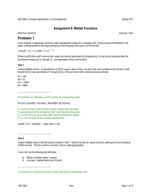
CEE 3804: Computer Applications in Civil Engineering Spring 2011<br />
Date Due: Solutions<br />
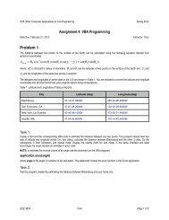
<strong>Problem</strong> 1<br />
<strong>Assignment</strong> 6: <strong>Matlab</strong> <strong>Functions</strong><br />
Instructor: Trani<br />
A civil engineer is designing a rainstorm water management system for a shopping mall. During a severe thunderstorm, the<br />
water runoff generated by the large parking lot at the shopping mall is given by the function:<br />
runoff = k 2<br />
+ k 1<br />
sin(t / k 3<br />
)e (−t /k 4 )<br />
Where runoff is the runoff volume (cubic meters per second) generated by the parking lot, t is the time (in seconds) after the<br />
thunderstorm starts and k 1<br />
through k 4<br />
are parameters of the runoff function.<br />
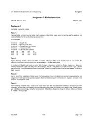
Task 1<br />
Create a <strong>Matlab</strong> function to calculate the runoff for a given value of time t. As part of the input variables to the function runoff,<br />
include the four input parameters k1 through k4 for a 100 year storm with numerical values as follows:<br />
k1 = 50;<br />
k2 = 2;<br />
k3 = 1500;<br />
k4 = 800;<br />
________________________<br />
% Function to estimate runoff volume at a shopping mall<br />
function [runoff] = function_Runoff(k1,k2,k3,k4,t)<br />
% runoff is the runoff volume (cubic meters per second)<br />
% generated by the shopping mall into the ponding area<br />
% t is the time (in seconds) after the thunderstorm starts<br />
% k1, k2, k3 and k4 are model coefficients.<br />
runoff = k1 * sin(t/k3) .* exp(-t/k4) + k2;<br />
________________________<br />
Task 2<br />
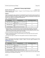
Create a <strong>Matlab</strong> script to call the function created in Task 1. Test the function for values of time (t) starting at t=0 and ending at<br />
t=4500 seconds. Plot the runoff as a function of time. Label appropriately.<br />
In your plot use the following plot attributes:<br />
a) Marker of plotted values = square<br />
b) Line type = dashed black line (10 point)<br />
________________________<br />
% Function to call the function runoff volume at a shopping mall<br />
CEE 3804 Trani Page 1 of 13
% Ponding volume at a shopping mall<br />
% Calls function Runoff<br />
clc<br />
clear<br />
% qRunoff is the runoff volume (cubic meters per second)<br />
% generated by the shopping mall into the ponding area<br />
% t is the time (in seconds) after the thunderstorm starts<br />
k1 = 50;<br />
k2 = 2;<br />
k3 = 1500;<br />
k4 = 800;<br />
tLast = 4500;<br />
% multiplicative parameter of the function<br />
% additive parameter of the function<br />
% parameter of sinusoidal term<br />
% parameter of exponential term<br />
% final time to do the calculation<br />
t=1:1:tLast; % create an array with values of time<br />
qRunoff(t) = function_Runoff(k1,k2,k3,k4,t);<br />
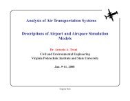
% Make a nice plot<br />
figure<br />
plot(t,qRunoff,'o')<br />
xlabel('Time (seconds)')<br />
ylabel('Volume (cu. meters/second)')<br />
grid<br />
% Make a plot of the derivative of runoff<br />
derQin = gradient(qRunoff);<br />
figure<br />
plot(t,derQin,'^')<br />
xlabel('Time (seconds)')<br />
ylabel('Gradient of qRunoff (cu. meters/second^2)')<br />
grid<br />
CEE 3804 Trani Page 2 of 13
Figure 1. Runoff Function.<br />
_______________________<br />
Task 3<br />
Modify the <strong>Matlab</strong> script created in Task 2 to find the area under the curve of the runoff as a function of time. Use the <strong>Matlab</strong><br />
“quad” function to estimate the integral. Plot the results and output the result of the area under the curve in the command window<br />
using the “disp” function in <strong>Matlab</strong>. How much runoff is produced in the 4500 second storm event? State the units of the answer.<br />
__________________________<br />
% Script to calculate the area under the runoff function<br />
% Programmer: T. Trani<br />
global k1 k2 k3 k4<br />
% Calls function function_Runoff_rev<br />
% areaUnderRunoff is the runoff volume (cubic meters per second)<br />
% generated by the shopping mall into the ponding area<br />
% t is the time (in seconds) after the thunderstorm starts<br />
k1 = 50;<br />
k2 = 2;<br />
k3 = 1500;<br />
k4 = 800;<br />
tLast = 4500;<br />
% multiplicative parameter of the function<br />
% additive parameter of the function<br />
% parameter of sinusoidal term<br />
% parameter of exponential term<br />
% final time to do the calculation (seconds)<br />
CEE 3804 Trani Page 3 of 13
% Estimate the area under runoff function<br />
areaUnderRunoff = quad('function_Runoff_rev',0,tLast);<br />
disp(['Area under the Curve is ',num2str(areaUnderRunoff)])<br />
______________________ function_Runoff_rev.m function ________<br />
% Function to estimate runoff volume at a shopping mall<br />
function [runoff] = function_Runoff_rev(t)<br />
global k1 k2 k3 k4<br />
% runoff is the runoff volume (cubic meters per second)<br />
% generated by the shopping mall into the ponding area<br />
% t is the time (in seconds) after the thunderstorm starts<br />
runoff = k1 * sin(t/k3) .* exp(-t/k4) + k2;<br />
________________________________<br />
Area under the Curve is 25652.45 cubic meters<br />
Task 4<br />
Estimate the dimensions of a ponding volume needed to store all the runoff volume generated by the 100 storm event. State<br />
dimensions of the ponding volume (base x width x height).<br />
One estimate of the ponding volume would be 100 x 100 x 2.57 meters. This is equivalent to two Football stadiums with<br />
a depth of 2.27 meters (8.5 feet).<br />
CEE 3804 Trani Page 4 of 13
<strong>Problem</strong> 2<br />
A train engineer collects data during the certification of the new high-speed train to be introduced in the Northeast Corridor in the<br />
United States. The data collected records train acceleration (a) vs. velocity (V). The data is presented in the table below.<br />
Table 1. Train Acceleration and Speed Data.<br />
Train Velocity (m/s)<br />
Maximum Train Acceleration<br />
(m/s 2 )<br />
0.00 3.51<br />
21.31 2.32<br />
30.40 1.73<br />
50.16 0.94<br />
69.65 0.39<br />
81.45 0.12<br />
94.20 0.01<br />
Task 1<br />
Create a <strong>Matlab</strong> script to plot the data and (in the same script) to find the best second and third order polynomials that fit the data<br />
(i.e., use the “polyfit” command). Save the coefficients of the polynomials and evaluate 100 data points of these polynomials<br />
across a range of speeds from 0-95 m/s (the usable operating speeds for this train). Compare with the original data.<br />
____________________________ <strong>Matlab</strong> Script for Task 1, <strong>Problem</strong> 2 ________________<br />
% <strong>Problem</strong> 2<br />
% Task 1<br />
% Data<br />
A=[0.00 3.51;21.31 2.32; 30.40 1.73; 50.16 0.94; 69.65 0.39; 81.45 0.12; 94.20 0.01];<br />
velocity=A(:,1);<br />
maxAcceleration=A(:,2);<br />
%% fitting to second order polynomial<br />
[p2,s2]=polyfit(velocity, maxAcceleration, 2);<br />
%% fitting to third order polynomial<br />
[p3, s3]=polyfit(velocity, maxAcceleration, 3);<br />
%% 100 data points for evaluating the two polynomials<br />
X=linspace(0,95,100);<br />
%% evaluating of second-order polynomial<br />
Y2=polyval(p2,X);<br />
CEE 3804 Trani Page 5 of 13
%% evaluating of third-order polynomial<br />
Y3=polyval(p3,X);<br />
% Make a good plot. We use the plot command with a variation (h = plot) to embellish the plot using<br />
% <strong>Matlab</strong> handle graphics<br />
h=plot(velocity,maxAcceleration,'ok',X,Y2,'b-',X,Y3,'r-');<br />
set(h, 'linewidth',2);<br />
set(gca, 'fontsize',20);<br />
title('Velocity-Maximum Acceleration Graph','fontsize',20);<br />
xlabel('Velocity (m/s)', 'fontsize',20);<br />
ylabel('Maximum Acceleration (m/s^2)', 'fontsize',20);<br />
legend('Observed data','Second-Order Polynomial','Third-Order Polynomial');<br />
grid on<br />
_____________________________________<br />
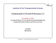
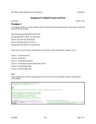
The <strong>Matlab</strong> script produces the graph shown in Figure 2.<br />
Figure 2. Plot of Train Acceleration Data vs. Speed.<br />
Task 2<br />
Using the best fit polynomials estimated in Task 1, evaluate the goodness of fit of both answers looking at the residuals or the<br />
local differences between the data points and the fitted polynomials. Select the best model fit. Comment on your solution.<br />
The script to find the residuals is:<br />
CEE 3804 Trani Page 6 of 13
%% task 2<br />
%% finding residuals<br />
normOfResiduals2=s2.normr;<br />
normOfResiduals3=s3.normr;<br />
Comparing normOfResiduals2 (2nd order polynomial) with norm of residuals for the third-order<br />
polynomial we conclude that the 3rd-order polynomial is closer to the data and hence a better<br />
model.<br />
The best fit equation of the 3rd-order polynomial is:<br />
a(t) = dV = k 1<br />
+ k 2<br />
V + k 3<br />
V 2 + k 4<br />
V 3<br />
dt<br />
where:<br />
k 4<br />
= 0.000000576703820<br />
k 3<br />
= 0.000235555589820<br />
k 2<br />
= -0.064571096680574<br />
k 1<br />
= 3.520152968080940<br />
Task 3 and <strong>Problem</strong> 3 (Task 1)<br />
Create another set of scripts (as needed) and using the best polynomial fit found in Task 2, solve the differential equation of<br />
motion for the train using the <strong>Matlab</strong> ODE45 solver. The equation of motion to estimate acceleration of the train is of the form:<br />
a(t) = dV<br />
dt<br />
= k 1<br />
+ k 2<br />
V + k 3<br />
V 2 + k 4<br />
V 3<br />
where: a(t) = dV is the instantaneous train acceleration (m/s 2 ), V is the train speed (m/s) and parameters k 1<br />
,k 2<br />
,k 3<br />
,k 4<br />
dt<br />
are the coefficients of the polynomial found in Task 2.<br />
Solve the differential equation with initial conditions V 0<br />
and a final time of 120 seconds. Plot the velocity and acceleration<br />
profiles in a 2 x1 window using the <strong>Matlab</strong> subplot command.<br />
_______________ Main <strong>Matlab</strong> Script to Estimate Train Speed and Distance Profiles ___________<br />
% Main file to find speed and distance traveled profile for a high-speed<br />
% rail system<br />
% This functions calls: trainFunction.m which contains rates of change of the velocity and distance state<br />
% variables of the train as a function of time<br />
% Define the following:<br />
% yprime(1) = acceleration<br />
% yprime(2) = speed<br />
% yprime(1) = k1 + k2 * y(1) + k3 * y(1)^2 + k4 * y(1) ^3<br />
% yprime(2) = y(1)<br />
CEE 3804 Trani Page 7 of 13
% y(1) = velocity (m/s)<br />
% y(2) = distance traveled (m)<br />
global k1 k2 k3 k4<br />
% Define Initial Conditions of the <strong>Problem</strong><br />
yo = [0 0];<br />
to = 0.0;<br />
tf = 120;<br />
% yo are the initial speed and distance traveled<br />
% to is the initial time to solve this equation<br />
% tf is the final time<br />
% define constants k1 - k4 (obtained from regression analysis)<br />
k1 = 3.520152968080940;<br />
k2 = -0.064571096680574;<br />
k3 = 0.000235555589820;<br />
k4 = 0.000000576703820;<br />
tspan =[to tf];<br />
[t,y] = ode45('trainFunction',tspan,yo);<br />
% call ODE solver<br />
% Plot the results of the numerical integration procedure<br />
subplot(2,1,1) % plots time-distance traveled profile<br />
h1 = plot(t,y(:,2),'^--b'); % gets handle graphics<br />
set(h1, 'linewidth',1); % sets the line width to 1<br />
set(gca, 'fontsize',20); % sets the font size to 20<br />
xlabel('Time (seconds)')<br />
ylabel('Distance Traveled (m)')<br />
grid<br />
subplot(2,1,2) % plots time-speed profile<br />
h2 = plot(t,y(:,1),'o--r')<br />
set(h2, 'linewidth',1); % sets the line width to 1<br />
set(gca, 'fontsize',20); % sets the font size to 20<br />
xlabel('Time (seconds)')<br />
ylabel('Speed (m/s)')<br />
grid<br />
CEE 3804 Trani Page 8 of 13
______________ Function trainFunction.m _____________________<br />
function yprime=trainFunction(t,y)<br />
% Define the following:<br />
% yprime(1) = acceleration<br />
% yprime(2) = speed<br />
% yprime(1) = k1 + k2 * y(1) + k3 * y(1)^2 + k4 * y(1) ^3<br />
% yprime(2) = y(1)<br />
% y(1) = velocity (m/s)<br />
% y(2) = distance traveled (m)<br />
global k1 k2 k3 k4<br />
yprime(1) = k1 + k2 * y(1) + k3 * y(1).^2 + k4 * y(1).^3; % finds acceleration<br />
yprime(2)= y(1);<br />
yprime = yprime';<br />
_______________________________<br />
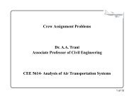
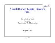
Execution of the Main file in <strong>Matlab</strong> produces:<br />
CEE 3804 Trani Page 9 of 13
Figure 3. High-Speed Train Distance and Speed Profiles. Note: the train reaches 80 m/s (180 mph) in around 100 seconds after<br />
start.<br />
CEE 3804 Trani Page 10 of 13
<strong>Problem</strong> 3<br />
Task 2<br />
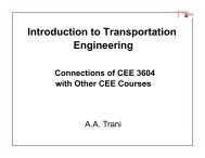
Solve the train problem using Simulink. Create a Simulink model to estimate the acceleration, velocity and distance profiles of<br />
the train as a function of time using the best fit polynomial model found in Task 2 of <strong>Problem</strong> 2.<br />
Equation to be modeled in Simulink.<br />
a(t) = dV<br />
dt<br />
= k 1<br />
+ k 2<br />
V + k 3<br />
V 2 + k 4<br />
V 3<br />
Figure 4. Simulink Model of the High-Speed Train. Third-Order Polynomial.<br />
CEE 3804 Trani Page 11 of 13
Task 3<br />
Export the results obtained by the Simulink model created in Task 2 and plot in <strong>Matlab</strong>. Label all the axes as needed. Simulink<br />
plots are not acceptable.<br />
__________________ <strong>Matlab</strong> Script to Plot Simulink Results obtained from the Workspace _______<br />
% Script to plot the results of a simulink model<br />
% Simulink model outputs:<br />
% tout = time signal (seconds) for state variables (speed and distance)<br />
% xout = state variables (speed and distance)<br />
% xout(:,1) = speed (m/s)<br />
% xout(:,2) = distance (m)<br />
% Acceleration = output of acceleration time trace (m/s-s)<br />
! % NOTE: Acceleration by default is a structured array<br />
! % Plot Acceleration.signals.values<br />
subplot(3,1,1) % plots time-acceleration profile<br />
h3 = plot(tout,Acceleration.signals.values,'*--k')<br />
set(h3, 'linewidth',1); % sets the line width to 1<br />
set(gca, 'fontsize',20); % sets the font size to 20<br />
xlabel('Time (seconds)')<br />
ylabel('Acceleration (m/s-s)')<br />
grid<br />
subplot(3,1,2) % plots time-speed profile<br />
h2 = plot(tout,xout(:,1),'o--r')<br />
set(h2, 'linewidth',1); % sets the line width to 1<br />
set(gca, 'fontsize',20); % sets the font size to 20<br />
xlabel('Time (seconds)')<br />
ylabel('Speed (m/s)')<br />
grid<br />
subplot(3,1,3) % plots time-distance traveled profile<br />
h1 = plot(tout,xout(:,2),'^--b'); % gets handle graphics<br />
set(h1, 'linewidth',1); % sets the line width to 1<br />
set(gca, 'fontsize',20); % sets the font size to 20<br />
xlabel('Time (seconds)')<br />
ylabel('Distance Traveled (m)')<br />
grid<br />
CEE 3804 Trani Page 12 of 13
Figure 5. Plot of Acceleration, Speed and Distance Traveled by High-Speed Train.<br />
CEE 3804 Trani Page 13 of 13