2 - People.stat.sfu.ca

STAT 801
Solutions: Asst 2
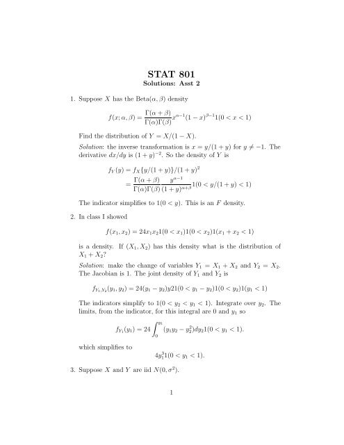
1. Suppose X has the Beta(α, β) density
f(x; α, β) =
Find the distribution of Y = X/(1 − X).
Γ(α + β)
Γ(α)Γ(β) xα−1 (1 − x) β−1 1(0 < x < 1)
Solution: the inverse transformation is x = y/(1 + y) for y ≠ −1. The
derivative dx/dy is (1 + y) −2 . So the density of Y is
f Y (y) = f X {y/(1 + y)}/(1 + y) 2
=
Γ(α + β) y α−1
1(0 < y/(1 + y) < 1)
Γ(α)Γ(β) (1 + y)
α+β
The indicator simplifies to 1(0 < y). This is an F density.
2. In class I showed
f(x 1 , x 2 ) = 24x 1 x 2 1(0 < x 1 )1(0 < x 2 )1(x 1 + x 2 < 1)
is a density. If (X 1 , X 2 ) has this density what is the distribution of
X 1 + X 2 ?
Solution: make the change of variables Y 1 = X 1 + X 2 and Y 2 = X 2 .
The Jacobian is 1. The joint density of Y 1 and Y 2 is
f Y1 ,Y 2
(y 1 , y 2 ) = 24(y 1 − y 2 )y21(0 < y 1 − y 2 )1(0 < y 2 )1(y 1 < 1)
The indicators simplify to 1(0 < y 2 < y 1 < 1). Integrate over y 2 . The
limits, from the indicator, for this integral are 0 and y 1 so
which simplifies to
f Y1 (y 1 ) = 24
∫ y1
3. Suppose X and Y are iid N(0, σ 2 ).
0
(y 1 y 2 − y 2 2 )dy 21(0 < y 1 < 1).
4y 3 1 1(0 < y 1 < 1).
1

(a) Show that X 2 + Y 2 and X/(X 2 + Y 2 ) 1/2 are independent.
The event U ≡ X 2 + Y 2 < u and −1 < T ≡ X/(X 2 + Y 2 ) 1/2 ≤ t
can be written in polar co-ordinates as r 2 ≤ u and −1 < cos θ ≤ t.
Let A denote this set of (x, y) pairs in the xy plane. Then
∫
P ((X, Y ) ∈ A) =
A
e −(x2 +y 2 )/2
2π
dxdy
which can be transformed to polar co-ordinates. The limits on r
will be 0 and u 1/2 . To get the limits on θ you have to remember
that the cosine is negative from π/2 to 3π/2 and so you integrate
from arccos(t) (a number between 0 and π as I define it here) to
2π − arccos(t). You get
P ((X, Y ) ∈ A) =
∫ u 1/2 ∫ 2π−arccos(t)
e −r2 /2
0
arccos(t)
which becomes
∫ u 1/2
2(π − arccos(t)) re −r2 /2 dr/(2π)
0
Do the integral to get
dθrdr/(2π)
P (U ≤ u, T ≤ t) = [1 − arccos(t) ](1 − e −u/2 )
π
for u > 0 and −1 ≤ t ≤ 1. This factors so that U and T are
independent. The cdf of T is thus
for −1 ≤ t ≤ 1.
F T (t) = 1 − arccos(t)
π
(b) Show that Θ = arcsin(X/(X 2 + Y 2 ) 1/2 ) is uniformly distributed
on (−π/2, π/2].
2

We have, for π/2 ≤ θ ≤ π/2,
P (Θ ≤ θ) =P (arcsin(T ) ≤ θ)
=P (T ≤ sin(θ))
=1 − arccos(sin(θ))
π
arccos(cos(θ − π/2))
=1 −
π
arccos(cos(π/2 − θ))
=1 −
π
= 1 − π/2 − θ
π
= (θ + π/2)/π
which is the cdf of the required distribution.
(c) Show X/Y is a Cauchy random variable.
Suppose z > 0. The event X/Y ≤ z corresponds to the region
y > 0 and x < zy together with the region y < 0 and x > zy. In
polar co-ordinates this has 0 < r < ∞ and either
or
We get
P (X/Y ≤ z) =
which is just
tan −1 (1/z) ≤ θ ≤ π/2
tan −1 (1/z) + π ≤ θ ≤ 3π/2
∫ ∞
0
e −r2 /2 rdr
[ ∫ π/2
tan −1 (1/z)
∫ ]
3π/2
dθ
+
tan −1 (1/z)+π 2π
2(π/2 − tan −1 (1/z))
2π
Differentiate to get the density
= 1/2 − tan −1 (1/z)/π
f(z) =
3
1
π(1 + z 2 ) .

4. Suppose X is Uniform on [0,1] and Y = sin(4πX). Find the density of
Y .
Solution: This transformation is many to 1. For each y ∈ (−1, 1) there
are 4 corresponding x values which map to y. The density of Y is
∑
1/|dy/dx|
x:sin(4πx)=y
We find dy/dx = 4π cos(x) and |dy/dx| = 4π √ 1 − sin 2 (x). Evaluated
at any x for which sin(4πx) = y this is 4π √ 1 − y 2 . This makes
1
f Y (y) = 4
4π √ 1 − y 1(−1 < y < 1) = 1
2 π √ 1(−1 < y < 1).
1 − y2 5. Suppose X and Y have joint density f(x, y). Prove from the definition
of density that the density of X is g(x) = ∫ f(x, y) dy.
Solution: I defined g to be the density of X provided
∫
P (X ∈ A) = g(x)dx
but
∫
A
∫
g(x)dx =
∫
=
A
∫
A×(−∞,∞)
A
f(x, y) dydx
f(x, y)dxdy
= P ((X, Y ) ∈ A × (−∞, ∞))
= P (X ∈ A)
Notice that I have used the fact that f is the density of (X, Y ) in the
middle of this.
6. Suppose X is Poisson(θ). After observing X a coin landing Heads with
probability p is tossed X times. Let Y be the number of Heads and Z
be the number of Tails. Find the joint and marginal distributions of Y
and Z.
4

Solution: Start with the joint:
P (Y = y, Z = z) = P (X = y + z, Y = y)
= P (Y = y|X = y + z)P (X = y + z)
( )
y + z
=
p y (1 − p) y+z−y exp(−λ)λ y+z /(y + z)!
y
= (pλ) y exp(−λp)[(1 − p)λ] z exp(−(1 − p)λ)/(y!z!)
which clearly factors into the product of two Poisson probability mass
functions. Thus Y and Z are independent Poissons with means pλ and
(1 − p)λ.
7. Let p 1 be the bivariate normal density with mean 0, unit variances and
correlation ρ and let p 2 be the standard bivariate normal density. Let
p = (p 1 + p 2 )/2.
(a) Show that p has normal margins but is not bivariate normal.
The margins of p are the averages of the margins of p 1 and p 2 .
In class I told you the margins of normals are normal so you
only need to know the means and variances of the margins to see
which normal. Both p 1 and p 2 have means 0 and variances 1 so the
margins are standard normal. Thus the margins of p are standard
normal. It follows that p has means 0 and variances 1. If p were
bivariate normal it would have to have correlation ρ/2 (to see this
compute corr = ∫ ∫ xyp(x, y)dx dy). Now check that at x = 0,
y = 0 p(0, 0) is not equal to the density of a bivariate normal with
mean 0, variances 1 and correlation ρ/2. Easier to check is this:
E(X 2 Y 2 ) = [E 1 (X 2 Y 2 ) + E 2 (X 2 Y 2 )]/2
But if (X, Y ) has density p 1 then the conditional distribution of
Y given X = x is N(ρx, 1 − ρ 2 ) so
and
E(Y 2 |X) = V ar(Y |X) + E 2 (Y |X) = 1 − ρ 2 + ρ 2 X 2
E(X 2 Y 2 ) = E[X 2 E(Y 2 |X)]
= E[X 2 (1 − ρ 2 + ρ 2 X 2 )
= 1 − ρ 2 + ρ 2 E(X 4 )
= 1 + 2ρ 2
5

Since p 2 is a special case of p 1 with ρ = 0 we find
which is not
unless ρ = 0.
E(X 2 Y 2 ) = [1 + 2ρ 2 + 1]/2 = 1 + ρ 2
E ρ/2 (X 2 Y 2 ) = 1 + 2(ρ/2) 2 = 1 + ρ 2 /2
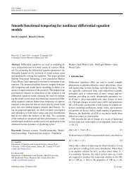
(b) Generalize the construction to show that there rv’s X and Y such
that X and Y are each standard normal, X and Y are uncorrelated
but X and Y are not independent.
Define p 1 as in the first part and p 2 like p 1 but with correlation
−ρ. The density p = (p 1 + p 2 )/2 has standard normal margins
and correlation 0 but does not factor. In this case
E(X 2 Y 2 ) = 1 + 2ρ 2 ≠ 1
unless ρ = 0. Here is a contour plot of the joint density when
ρ = 0.8.
6

y
-3 -2 -1 0 1 2 3
-3 -2 -1 0 1 2 3
x
8. Suppose X and Y are independent with X ∼ N(µ, σ 2 ) and Y ∼
N(γ, τ 2 ). Let Z = X + Y . Find the distribution of Z given X and that
of X given Z.
7

I intended you to: find the joint density of X, Z by change of variables,
and then divide joint by marginal to get the conditional densities.
Here is one way to do part of the problem. Consider first the following
problem: U, V are bivariate normal with mean 0 and variance covariance
matrix [
1
]
ρ
ρ 1
Then
f U,V (u, v) =
1
2π √ − 2ρuv + v 2
1 − ρ 2 exp{−u2 }
2(1 − ρ 2 )
Rewrite u 2 − 2ρuv + v 2 as (u − ρv) 2 + (1 − ρ 2 )v 2 to see that
f V (v) =
1
2π √ 1 − ρ 2 e−v2 /2
∫ ∞
−∞
e −(u−ρv)2 /[2(1−ρ 2 )] du
In the integral substitute y = (u − ρv)/ √ 1 − ρ 2 and find that
f V (v) = 1 √
2π
e −v2 /2
The conditional density of U given V = v is then
f U|V (u|v) = f U,V (u, v)
f V (v)
which is the N(ρv, 1 − ρ 2 ) density.
√
(u − ρv)2
= exp{−
2(1 − ρ 2 ) − v2
2 + v2 2π
2 } 2π
= exp{−(u − ρv) 2 /[2(1 − ρ 2 )]}/ √ 2π(1 − ρ 2 )
Now if X = σU + µ and Z = φV + µ + γ then X, Z has the joint
distribution of X and X + Y of the original problem provided we make
ρ = Corr(X, Z). For X and Z as in the problem we find φ 2 = σ 2 + τ 2 ,
the covariance is σ 2 , and the correlation is
ρ =
1
√
1 + τ
2
/σ 2 =
σ
√
σ2 + τ 2 = σ φ
8

Thus X, Z is a change of variables from U, V . We get
f X,Z (x, z) = 1
σφ f U,V [(x − µ)/σ, (z − µ − γ)/φ]
and
so that
f Z (z) = 1 φ f V [(z − µ − γ)/φ]
f X|Z (x|z) = 1 σ f U|V ([(x − µ)/σ, (z − µ − γ)/φ]
Plug in to the formula for f U|V
to get
f X|Z (x|z) =
The exponent is
1
σ √ 1 − ρ 2 exp{−[(x−µ)/σ −ρ((z −µ−γ)/φ]2 /[2(1−ρ 2 )]}
[x − µ − ρσ(z − µ − γ)/φ]2
−
2σ 2 (1 − ρ 2 )
which means that the conditional distribution of X given Z = z is
normal with mean
σ
µ + ρ√ (z − µ − γ) = µ +
σ2
(z − µ − γ)
σ2 + τ
2 σ 2 + τ
2
and variance
σ 2 (1 − ρ 2 ) = σ2 τ 2
σ 2 + τ 2
9