Mass Transfer Between a Sphere and an Unbounded Fluid ( )

Mass Transfer Between a Sphere and an Unbounded Fluid
R. Shankar Subramanian
Department of Chemical and Biomolecular Engineering
Clarkson University
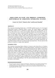
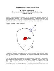
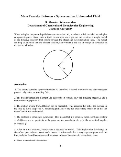
When a single-component liquid drop evaporates into air, or when a solid, modeled as a singlecomponent
sphere, dissolves in a liquid or sublimes into a gas, we can construct a simple model
of the diffusive transport that occurs between the object and the surrounding fluid. The model
can help us calculate the rate of mass transfer, and eventually the rate of change of the radius of
the sphere with time.
r
a
Assumptions
1. The sphere contains a pure component A; therefore, we need to consider the mass transport
process only in the surrounding fluid.
2. The fluid is unbounded in extent and quiescent. It contains only the diffusing species A and a
non-transferring species B.
3. The motion arising from diffusion can be neglected. This requires that either the mixture in
the fluid be dilute in species A, consisting primarily of the non-transferring species B, or that the
rate of mass transport be small.
4. The problem is spherically symmetric. This means that in a spherical polar coordinate system
( r, θφ , ) there are no gradients in the polar angular coordinate θ , or in the azimuthal angular
coordinate φ .
5. After an initial transient, steady state is assumed to prevail. This implies that the change in
size of the sphere due to mass transfer occurs on a time scale that is very large compared with the
time scale for the diffusion process for a given radius of the sphere to reach steady state.
6. There are no chemical reactions.
1

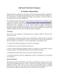
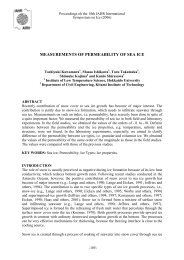
Because there are no gradients in the θ and φ directions, and there is no time-dependence, the
flux N
Ar
depends only on r . At steady state the rate at which species A enters the spherical
shell shown at location r must equal the rate at which species A leaves the shell at r+∆ r .
r
∆r
a
Using the standard symbol for the molar flux of A at these two locations, we can write the steady
state conservation of mass statement as
2
( ) π ( ) ( )
πr N r − r+∆ r N r+∆ r =
2
4
A
4 0
r
Ar
Dividing through by the factor 4π∆ r , and rearranging yields
( r r) 2 N ( r r) r 2 N ( r)
+∆
A
+∆ − 0
r
A
=
r
∆r
Taking the limit as ∆r
→ 0 leads to the ordinary differential equation
d
rNAr
dr
2
( )
= 0
We can integrate this immediately to obtain
2
rNAr
C1
= C1
, which can be recast as NAr
( r) =
2
r
where C
1
is an arbitrary constant of integration. Now, we proceed to use Fick’s law.
dx
( )
A
NAr = xA NAr + NBr − cDAB
dr
2

The first term in the right side corresponds to convective transport, which can be neglected in
this problem because of assumptions 2 and 3. Thus, we obtain the following first order ordinary
differential equation for the mole fraction of species A in the fluid.
dxA
C1
1
= −
2
dr c D r
AB
Integration of this equation is straightforward, and leads to the following solution.
C1
1
xA
( r) = + C
cD r
AB
2
There are two arbitrary constants that need to be evaluated. Therefore, we must write two
boundary conditions. At the surface of the sphere, we can assume equilibrium to prevail
between the two phases. For example, if species A is evaporating into a gas, the partial pressure
of species A in the gas phase at the interface can be assumed to be equal to its equilibrium vapor
pressure at the prevailing temperature. If the gas mixture is assumed ideal, then the mole
fraction of species A in the gas phase at the interface is the ratio between this equilibrium vapor
pressure of A and the prevailing total pressure in the gas phase. In non-ideal cases, a
corresponding result can be used to obtain the equilibrium mole fraction of species A in the gas
phase at the interface. Likewise, for a solid dissolving in a liquid, or subliming into a gas, the
equilibrium mole fraction of species A in the fluid at the interface can be obtained.
A
( ) =
A1
x a x
Far from the sphere, we can assume the composition to approach that in the fluid in the absence
of the sphere. Thus,
xA
( ∞ ) = 0
Application of these two boundary conditions permits us to evaluate the constants C
1
and C
2
as
C = cD ax
C
2
= 0
1 AB A1
Substituting these results in the solution leads to the following result for the radial distribution of
the mole fraction of species A in the fluid.
( )
xA
r a
=
x r
A1
The flux of species A is given by
3

1
r
( ) =
1 2
N r cD ax
Ar AB A
so that the molar rate of mass transfer at the surface of the sphere can be written as
( )
W = πa N a = π c D a x = π D ac
2
A
4
Ar
4
AB A1 4
AB A1
where we have used the fact that the product cxA
1
= cA
1, the molar concentration of A in the
fluid at the interface. Assuming that the molar rate of transport is relatively small, we can use a
mass balance on the sphere to deduce the rate of change of its size with time. Let the molecular
weight of A be M , and the density of the sphere be ρ . Then, we can write
A
d ⎛4
da
dt 3
π ρ ⎞
⎜ ⎟ = π ρ = −
⎝ ⎠ dt
π
3 2
a 4 a 4 DAB MA acA
1
which leads to a differential equation for the time-dependence of the radius of the sphere.
da
a dt
= −
DAB M
A
cA1
ρ
If the radius at time zero is a
0
, then the solution can be written as
2 2 2 D
1
( )
AB
M A
c
= A
0
−
a t a t
ρ
The Quasi-Steady State Assumption
Note that we assumed steady state to prevail in the diffusion problem, which, strictly speaking,
requires the size of the sphere to remain unchanged. As stated in assumption 5, this only requires
that the time scale over which the sphere changes appreciably in size be large compared with the
time scale over which the diffusion process around a sphere of constant size reaches steady state.
Then, the rate of mass transfer from the sphere to the fluid can actually be used to calculate the
time evolution of the size of the sphere. This type of assumption is called a quasi-steady state
assumption. We can make a judgment about whether it is a good assumption in a given situation
by comparing these two time scales. The time needed for the diffusion process around a sphere
2
of radius a
0
to reach steady state is approximately of the same order of magnitude as a / 0
D
AB
.
By estimating the time it takes for the sphere to completely dissolve in the fluid, we can get an
idea about the time scale for the size to change appreciably. From the equation for the radiustime
history of the sphere, this time scale is found to be of the order of magnitude of
2
ρa0
, where we have discarded the factor 2, because this is only an order of magnitude
D M c
AB A A1
4

estimate. Using these results, the following estimate can be obtained for the ratio of the two
time scales.
Time for diffusion process to attain steady state a / D M c
= =
Time for sphere to change in size appreciably ρa / D M c
2
0 AB A A1
2
0 ( AB A A1)
ρ
Therefore, in this problem, assumption 5 would be valid when the dimensionless group
M c ρ .
( A A1 ) / 1
The quasi-steady state assumption is invoked commonly in problems where there are two very
different time scales involved. For example, we can use the quasi-steady assumption in the
problem of calculating the rate of change of the height of liquid in a large storage tank through a
small pipe at the bottom. To calculate the velocity of flow out of the pipe and therefore the
volumetric flow rate, we can assume the level of the fluid in the tank to remain constant. After
obtaining such a volumetric flow rate from a steady-state model, it can be used in an unsteady
mass balance on the contents of the tank to calculate the rate of change of height of the liquid in
the tank.
5