Uncertainty and Risk - DARP

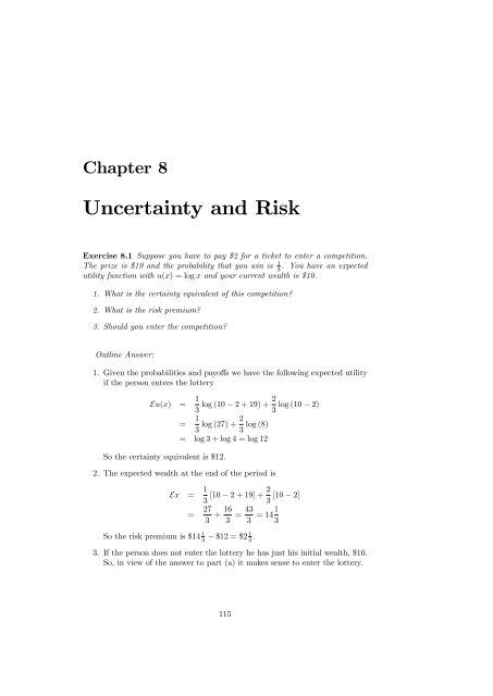
Chapter 8 

Uncertainty and Risk 

Exercise 8.1 Suppose you have to pay $2 for a ticket to enter a competition. 

The prize is $19 and the probability that you win is 1 3 

. You have an expected 

utility function with u(x) = log x and your current wealth is $10. 

1. What is the certainty equivalent of this competition? 

2. What is the risk premium? 

3. Should you enter the competition? 

Outline Answer: 

1. Given the probabilities and payo¤s we have the following expected utility 

if the person enters the lottery 

Eu(x) = 1 3 log (10 2 + 19) + 2 log (10 2) 

3 

= 1 3 log (27) + 2 log (8) 

3 

= log 3 + log 4 = log 12 

So the certainty equivalent is $12. 

2. The expected wealth at the end of the period is 

Ex = 1 3 [10 2 + 19] + 2 [10 2] 

3 

= 27 3 + 16 3 = 43 

3 = 141 3 

So the risk premium is $14 1 3 

$12 = $2 1 3 . 

3. If the person does not enter the lottery he has just his initial wealth, $10. 

So, in view of the answer to part (a) it makes sense to enter the lottery. 

115

Microeconomics CHAPTER 8. UNCERTAINTY AND RISK 

Exercise 8.2 You are sending a package worth 10 000AC. You estimate that 

there is a 0.1 percent chance that the package will be lost or destroyed in transit. 

An insurance company o¤ers you insurance against this eventuality for a 

premium of 15AC. If you are risk-neutral, should you buy insurance? 


No you should not. Your expected loss is 10 euros whereas the premium is 

15 euros. 

cFrank Cowell 2006 116

Microeconomics 

Exercise 8.3 Consider the following de…nition of risk aversion. Let P := 

f(x ! ; ! ) : ! 2 g be a random prospect, where x ! is the payo¤ in state ! 

and ! is the (subjective) probability of state ! , and let Ex := P !2 !x ! , 

the mean of the prospect, and let P := f(x ! + [1 ]Ex; ! ) : ! 2 g be a 

“mixture” of the original prospect with the mean. De…ne an individual as risk 

averse if he always prefers P to P for 0 < < 1. 

1. Illustrate this concept in (x red ; x blue )-space and contrast it with the concept 

of risk aversion used in the text 

2. Show that this de…nition of risk aversion need not imply convex-to-theorigin 

indi¤erence curves. 


1. See Figure 8.1. 

x BLUE 

P 

P λ 

P 

x RED 

Figure 8.1: Nonconvex indi¤erence curve 

2. Let P be the prospect and P its mean. P can be any point in the line 

joining them. The de…nition implies that moving along this line towards 

P puts the person on a successively higher indi¤erence curves. In Figure 

8.1 it is clear that this condition is consistent with there being indi¤erence 

curves that violate the convex-to-the-origin property locally. 



Exercise 8.4 Suppose you are asked to choose between two lotteries. In one 

case the choice is between P 1 and P 2 ;and in the other case the choice o¤ered is 

between P 3 and P 4 , as speci…ed below: 

P 1 : $1; 000; 000 with probability 1 

8 

< 

P 2 : 

P 3 : 

P 4 : 

$5; 000; 000 

$1; 000; 000 

: 

$0 

$5; 000; 000 

$0 

$1; 000; 000 

$0 

with probability 0.1 







It is often the case that people prefer P 1 to P 2 and then also prefer P 3 to P 4 . 

Show that these preferences violate the independence axiom. 


Let there be only three possible states of the world: red, blue and green, 

with probabilities 0.01, 0.10, 0.89 respectively. Then the payo¤s in the four 

prospects can be written 

red blue green 

P 1 1 1 1 

P 2 0 5 1 

P 3 0 5 0 

P 4 1 1 0 

where all the entries in the table are in millions of dollars. Note that P 1 and P 2 

have the same payo¤ in the green state; P 3 and P 4 form a similar pair, except 

that the payo¤ in the green state is 0. Axiom 8.2 states that if P 1 is preferred 

to P 2 than any other similar pair of prospects (1; 1; z) and (0; 5; z) ought also 

to be ranked in the same order, for arbitrary z: but this would imply that P 4 

is preferred to P 3 , the opposite of the preferences as stated. 

Note also that if the preferences had been such that P 4 was preferred to P 3 

then the independence axiom would imply that P 1 was preferred to P 2 . 



Exercise 8.5 This is an example to illustrate disappointment. Suppose the 

payo¤s are as follows 

x 00 weekend for two in your favourite holiday location 

x 0 book of photographs of the same location 

x …sh-and-chip supper 

Your preferences under certainty are x 00 x 0 x . Now consider the following 

two prospects 

8 

< x 00 

P 1 : 

: 

x 0 with probability 0 

P 2 : 

8 

< 

with probability 0:99 

x with probability 0:01 

x 00 with probability 0:99 


: 

x with probability 0 

Suppose a person expresses a preference for P 1 over P 2 . Brie‡y explain why 

this might be the case in practice. Which of the three axioms State Irrelevance, 

Independence, Revealed Likelihood, is violated by such preferences? 


It is possible that, given the information that the …rst event (with payo¤ x 00 ) 

has not happened you would then prefer x to x 0 : photographs of your favourite 

holiday spot may be too painful once you know that the holiday is not going to 

happen. So you may prefer P 1 over P 2 . 

These preferences violate the independence axiom. To see this, note that, 

by the revealed likelihood axiom, since x 0 is strictly preferred to x , it must be 

the case that P2 0 is strictly preferred to P1, 0 where 

P 0 1 : 

P 0 2 : 

x 

0 

with probability 0 


x 

0 



But P1 0 and P2 0 can be written equivalently as 

8 

< x 

P1 0 : x 0 with probability 0 

: 

P 0 2 : 

8 

< 





: 


By the independence axiom if P 0 2 is strictly preferred to P 0 1, then P 2 must be 

strictly preferred to P 1 . 



Exercise 8.6 An example to illustrate regret. Let 

P := f(x ! ; ! ) : ! 2 g 

P 0 := f(x 0 !; ! ) : ! 2 g 

be two prospects available to an individual. De…ne the expected regret if the 

person chooses P rather than P 0 as 

X 

! max fx 0 ! x ! ; 0g (8.1) 

!2 

Now consider the choices amongst prospects presented in Exercise 8.4. Show 

that if a person is concerned to minimise expected regret as measured by (8.1), 

then it is reasonable that the person select P 2 when P 1 is also available and then 

also select P 4 when P 3 is available. 


Denote the regret in (8.1) by r (P; P 0 ). 

If I choose P 2 when P 1 is also available then the regret is 

r (P 2 ; P 1 ) = 0:1 [0] + 0:89 [0] + :01 [1] 

= 10; 000 

Whereas, had I chosen P 1 when P 2 was available, then the regret would have 

been 

r (P 1 ; P 2 ) = 0:1 [4; 000; 000] + 0:89 [0] + :01 [0] 

= 400; 000 

If I choose P 4 when P 3 is also available then the regret is 

r (P 4 ; P 3 ) = 0:1 [0] + 0:89 [0] + :01 [0] 

= 0 

Whereas, had I chosen P 3 when P 4 was available, then the regret would have 

been 

r (P 3 ; P 4 ) = 0:1 [0] + 0:89 [0] + :01 [5; 000; 000] 

= 50; 000 



Exercise 8.7 An example of the Ellsberg paradox . There are two urns marked 

Left and Right each of which contains 100 balls. You know that in Urn L 

there exactly 49 white balls and the rest are black and that in Urn R there are 

black and white balls, but in unknown proportions. Consider the following two 

experiments: 

1. One ball is to be drawn from each of L and R. The person must choose 

between L and R before the draw is made. If the ball drawn from the chosen 

urn is black there is a prize of $1000, otherwise nothing. 

2. Again one ball is to be drawn from each of L and R; again the person must 

choose between L and R before the draw. Now if the ball drawn from the 

chosen urn is white there is a prize of $1000, otherwise nothing. 

You observe a person choose Urn L in both experiments. Show that this 

violates the Revealed Likelihood Axiom. 

Outline Answer 

The implication of the revealed likelihood axiom is that there exist subjective 

probabilities ! . The result is proved by showing that it the stated behaviour 

is inconsistent with the existence of subjective probabilities. 

In this case the revealed likelihood axiom implies that for each urn there is 

a given subjective probability of drawing a black ball L (left-hand urn) and R 

(right-hand urn) such that preferences can be represented as 

v black (x black ; x white ) + [1 ] v white (x black ; x white ) (8.2) 

where = L or R and x black and x white are the payo¤s if a black ball or a 

white ball are drawn respectively. 

Note that the representation (8.2) does not impose either the State Irrelevance 

Axiom (which would require that v black () and v white () be the same 

function) or the Independence axiom (which would require that v black () be a 

function only of x black etc.). Nor does it impose the common-sense requirement 

that L = 0:49. All we need below is the very weak assumption that preferences 

are not perverse: 

v black (1000; 0) > v white (1000; 0) (8.3) 

and 

v black (0; 1000) < v white (0; 1000) (8.4) 

Condition (8.3) simply says that if the $1000 prize is attached to a black ball 

then the utility to be derived from having selected a black ball is higher than 

selecting a white ball; condition (8.4) is the counterpart when the prize attaches 

to the white ball.. 

Experiment 1 suggests that 

L v black (1000; 0) + [1 L ] v white (1000; 0) 

> R v black (1000; 0) + [1 R ] v white (1000; 0) (8.5) 



while experiment 2 suggests that 

L v black (0; 1000) + [1 L ] v white (0; 1000) 

> R v black (0; 1000) + [1 R ] v white (0; 1000) (8.6) 

We can see that (8.5) implies 

L [v black (1000; 0) v white (1000; 0)] > R [v black (1000; 0) v white (1000; 0)] 

from which we deduce that, given (8.3), L > R . 

However (8.5) implies 

L [v black (0; 1000) v white (0; 1000)] > R [v black (0; 1000) v white (0; 1000)] : 

So that, given (8.4), we would have L < R –a contradiction. 

revealed likelihood axiom must be violated. 

Therefore the 



Exercise 8.8 An individual faces a prospect with a monetary payo¤ represented 

by a random variable x that is distributed over the bounded interval of the real 

line [a; a]. He has a utility function Eu(x) where 

u(x) = a 0 + a 1 x 

and a 0 ; a 1 ; a 2 are all positive numbers. 

1 

2 a 2x 2 

1. Show that the individual’s utility function can also be written as '(Ex; var(x)). 

Sketch the indi¤erence curves in a diagram with Ex and var(x) on the 

axes, and discuss the e¤ect on the indi¤erence map altering (i) the parameter 

a 1 , (ii) the parameter a 2 . 

2. For the model to make sense, what value must a have? [Hint: examine 

the …rst derivative of u.] 

3. Show that both absolute and relative risk aversion increase with x. 


1. Clearly 

Eu(x) = a 0 + a 1 E(x) + a 2 

1 

2 [(E(x))2 var(x)]: 

Marginal utility is a 1 a 2 x: 

2. For this to be non-negative we must have E(x) a 1 =a 2 hence the indi¤erence 

curves are depicted with E(x) as good, var(x) as bad and 

MRS = 2 [a 1 =a 2 E(x)] : 

3. 

u x (x) = a 1 + a 2 x 

u xx (x) = a 2 

(x) = 

(x) = 

%(x) = 

where and 0 x x max := 

u xx (x) 

u x (x) = a 2 

a 1 + a 2 x 

1 

x max x 

1 

x max =x 1 

a1 

a 2 

: 



Exercise 8.9 A person lives for 1 or 2 periods. If he lives for both periods he 

has a utility function given by 

U (x 1 ; x 2 ) = u (x 1 ) + u (x 2 ) (8.7) 

where the parameter is the pure rate of time preference. The probability of 

survival to period 2 is , and the person’s utility in period 2 if he does not 

survive is 0. 

1. Show that if the person’s preferences in the face of uncertainty are represented 

by the expected-utility functional form 

X 

! u (x ! ) (8.8) 

!2 

then the person’s utility can be written as 

What is the value of the parameter 0 ? 

u (x 1 ) + 0 u (x 2 ) : (8.9) 

2. What is the appropriate form of the utility function if the person could live 

for an inde…nite number of periods, the rate of time preference is the same 

for any adjacent pair of periods, and the probability of survival to the next 

period given survival to the current period remains constant? 


1. Consider the person’s lifetime utility with the consumption x 1 and x 2 

in the two periods. If the person survives into the second period utility 

is given by u (x 1 ) + u (x 2 ) otherwise it is just u (x 1 ). Given that the 

probability of the event “survive to second period”is expected lifetime 

utility is 

[u (x 1 ) + u (x 2 )] + [1 ] u (x 1 ) : 

On rearranging we get 

in other words the form (8.9) with 0 = . 

u (x 1 ) + u (x 2 ) ; (8.10) 

2. Apply the argument to one more period. Now there is consumption 

x 1 ,x 2 ; x 3 in the three periods and the probability of surviving into period 

t + 1 given that you have made it to period t is still . Consider the 

situation of someone who survives to period 2. The person gets utility 

u (x 2 ) + u (x 3 ) (8.11) 

if he survives to period 3 and u (x 2 ) otherwise. His expected utility for 

the rest of his lifetime, contingent on having reached period 2 is therefore 

cFrank Cowell 2006 124 

[u (x 2 ) + u (x 3 )] + [1 ] u (x 2 ) 

= u (x 2 ) + u (x 3 ) (8.12)


So now view the situation from the position of the beginning of the lifetime. 

The person gets utility 

u (x 1 ) + [u (x 2 ) + u (x 3 )] (8.13) 

if he makes it through to period 2, where the expression in square brackets 

in (8.13) is just the rest-of-lifetime expected utility if you get to period 2, 

taken from (8.12); of course if the person does not survive period 1 he gets 

just u (x 1 ). So, using the same reasoning as before, from the standpoint 

of period 1 lifetime expected utility is now 

Rearranging this we have 

[u (x 1 ) + [u (x 2 ) + u (x 3 )]] 

+ [1 ] u (x 1 ) : 

u (x 1 ) + u (x 2 ) + 2 2 u (x 2 ) : (8.14) 

It is clear that the same argument could be applied to T > 2 periods and 

that the resulting utility function would be of the form 

u (x 1 ) + u (x 2 ) + 2 2 u (x 2 ) + ::: + T T u (x 2 ) : (8.15) 

In other words we have the standard intertemporal utility function with 

the pure rate of time preference replaced by the modi…ed rate of time 

preference 0 := . 



Exercise 8.10 A person has an objective function Eu(y) where u is an increasing, 

strictly concave, twice-di¤erentiable function, and y is the monetary value 

of his …nal wealth after tax. He has an initial stock of assets K which he may 

keep either in the form of bonds, where they earn a return at a stochastic rate 

r, or in the form of cash where they earn a return of zero. Assume that Er > 0 

and that Prfr < 0g > 0. 

1. If he invests an amount in bonds (0 < < K) and is taxed at rate t 

on his income, write down the expression for his disposable …nal wealth y, 

assuming full loss o¤set of the tax. 

2. Find the …rst-order condition which determines his optimal bond portfolio 

. 

3. Examine the way in which a small increase in t will a¤ect . 

4. What would be the e¤ect of basing the tax on the person’s wealth rather 

than income? 


1. Suppose the person puts an amount in bonds leaving the remaining 

K of assets in cash. Then, given that the rate of return on cash is 

zero and on bonds is the stochastic variable r, income is 

[K ] 0 + r = r 

If the tax rate is t then, given that full loss o¤set implies that losses and 

gains are treated symmetrically, disposable income is 

and (disposable) …nal wealth is 

[1 t] r 

x = [K ] + + [1 t] r 

[cash] [value of bonds] [income] 

= K + [1 t] r: (8.16) 

Note that x is a stochastic variable and could be greater or less than initial 

wealth K. 

2. The individual’s optimisation problem is to choose to maximise Eu(x). 

Using (8.16) the FOC for an interior solution is 

which implies 

E (u x (x) [1 t] r) = 0; 

E (u x (x)r) = 0: (8.17) 

Solving this determines = (t; K), the optimal bond purchases that 

depends on the tax rate and initial wealth as well as the distribution of 

returns and risk aversion. 



3. Take the FOC (8.17). Substituting for x from (8.16) and di¤erentiating 

with respect to t we get 

 

 

E u xx (x) r + @ 

@t [1 t] r r = 0; 

so that 

 

E 

u xx (x)r 2 

+ @ 

@t 

+ @ 

@t [1 

[1 t] = 0 

@ 

@t 

= 

 

t] = 0: 

 

1 t : 

An increase in the tax rate increases the demand for bonds. 

4. Final wealth is initial wealth plus income. If the tax is on wealth then 

disposable …nal wealth is 

x = [1 t] K + [1 t] r (8.18) 

instead of (8.16). Clearly the FOC (8.17) remains essentially unaltered 

(the new tax just reduces total wealth). Di¤erentiating the FOC with x 

de…ned by (8.18) we now …nd 

This implies 

E 

 

u xx (x) 

KE (u xx (x)r) + E 

K r + @ 

@t [1 

 

u xx (x)r 2 

 

t] r r = 0; 

+ @ 

@t [1 

 

t] = 0: 

 

K E (u xx(x)r) 

E (u xx (x)r 2 ) + @ [1 t] = 0: 

@t 

@ 

@t [1 

@ 

@t 

t] = + K E (u xx(x)r) 

E (u xx (x)r 2 ) : 

= 

1 t + K 

1 t 

E (u xx (x)r) 

E (u xx (x)r 2 ) : 

The …rst term on the right-hand side is positive; as for the second term, 

the denominator is negative and the numerator is positive, given DARA. 

So the impact of tax on bond-holding is now ambiguous. 



Exercise 8.11 An individual taxpayer has an income y that he should report to 

the tax authority. Tax is payable at a constant proportionate rate t. The taxpayer 

reports x where 0 x y and is aware that the tax authority audits some tax 

returns. Assume that the probability that the taxpayer’s report is audited is 

, that when an audit is carried out the true taxable income becomes public 

knowledge and that, if x < y, the taxpayer must pay both the underpaid tax and 

a surcharge of s times the underpaid tax. 

1. If the taxpayer chooses x < y, show that disposable income c in the two 

possible states-of-the-world is given by 

c noaudit = y tx; 

c audit = [1 t st] y + stx: 

2. Assume that the individual chooses x so as to maximise the utility function 

[1 ] u (c noaudit ) + u (c audit ) : 

where u is increasing and strictly concave. 

(a) Write down the FOC for an interior maximum. 

(b) Show that if 1 s > 0 then the individual will de…nitely underreport 

income. 

3. If the optimal income report x satis…es 0 < x < y: 

(a) Show that if the surcharge is raised then under-reported income will 

decrease. 

(b) If true income increases will under-reported income increase or decrease? 


If the individual reports x then he pays tax tx –i.e. he underpays an amount 

t [y x]. So 

1. If the under-reporting remains undetected then 

c noaudit = y tx 

and if the audit takes place then 

2. The individual maximises 

= y ty + t [y x] 

c audit = y tx [1 + s] t [y x] 

= [1 t st] y + stx 

Eu(c) = [1 ] u (y tx) + u ([1 t st] y + stx) 

Di¤erentiating this we have 

@Eu(c) 

@x 

= t [1 ] u c (y tx) + stu c ([1 t st] y + stx) 

where u c () denotes the …rst derivative of u. 



(a) If there is an interior maximum at x then the following FOC must 

hold 

[1 ] u c (y tx ) = su c ([1 t st] y + stx ) : 

(b) If the person reports fully then 

@Eu(c) 

@x = t [1 ] u c (y ty) + stu c ([1 t] y) 

x=y 

= [1 s] tu c (y ty) 

Given that t and u c are positive it is clear that the above expression 

is negative if 1 s > 0. Therefore the individual’s expected 

utility would increase if he reduced x below y. 

3. Di¤erentiating the FOC with respect to s and rearranging we get 

t [1 ] u cc (y tx ) @x s 2 tu cc ([1 t st] y + stx ) @x 

@s 

@s 

= u c ([1 t st] y + stx ) + st [x y] u cc ([1 t st] y + stx ) 

(a) Therefore 

where 

@x 

@s = u c (c audit ) + st [x y] u cc (c audit ) 

t 

(8.19) 

:= [1 ] u cc (y tx ) s 2 u cc ([1 t st] y + stx ) > 0 

Given that u c > 0, x < y and u cc < 0 it is clear that the numerator 

of (8.19) is positive.x increases with s so t [y x ] decreases. 

(b) Di¤erentiating the FOC with respect to y we get 

 

[1 ] u cc (y tx ) 

1 t @x 

@y 

= su cc ([1 t st] y + stx ) 

Therefore we have 

@ [y x ] 

@y 

[1 t st] + st @x 

@y 

@x 

@y = s [1 t st] u cc (c audit ) [1 ] u cc (c noaudit ) 

t [[1 ] u cc (c noaudit ) + s 2 u cc (c audit )] 

@ [y x ] 

@y 

 

: 

= 1 + s [1 t st] u cc (c audit ) [1 ] u cc (c noaudit ) 

[[1 ] tu cc (c noaudit ) + s 2 tu cc (c audit )] 

= 1 t 

t 

[1 ] u cc (c noaudit ) su cc (c audit ) 

[[1 ] u cc (c noaudit ) + s 2 u cc (c audit )] 

This is of ambiguous sign unless we assume DARA in which case it 

is positive. 



Exercise 8.12 A risk-averse person has wealth y 0 and faces a risk of loss 

L < y 0 with probability . An insurance company o¤ers cover of the loss at 

a premium > L. It is possible to take out partial cover on a pro-rata basis, 

so that an amount tL of the loss can be covered at cost t where 0 < t < 1. 

1. Explain why the person will not choose full insurance 

2. Find the conditions that will determine t , the optimal value of t. 

3. Show how t will change as y 0 increases if all other parameters remain 

unchanged. 


1. Consider the person’s wealth after taking out (partial) insurance cover 

using the two-state model (no loss;loss). If the person remained uninsured 

it would be (y 0 ; y 0 L); if he insures fully it is (y 0 ; y 0 ). So 

if he insures a proportion t for the pro-rata premium wealth in the two 

states will be 

which becomes 

([1 t] y 0 + t [y 0 ] ; [1 t] [y 0 L] + t [y 0 ]) 

So expected utility is given by 

Therefore 

@Eu 

@t 

(y 0 t; y 0 t [1 t] L) 

Eu = [1 ] u (y 0 t) + u (y 0 t [1 t] L) 

= [1 ] u y (y 0 t) + [L ] u y (y 0 t [1 t] L) 

Consider what happens in the neighbourhood of t = 1 (full insurance). 

We get 

@Eu 

@t = [1 ] u y (y 0 ) + [L ] u y (y 0 ) 

t=1 

= [L ] u y (y 0 ) 

We know that u y (y 0 ) > 0 (positive marginal utility of wealth) and, by 

assumption, L < . Therefore this expression is strictly negative which 

means that in the neighbourhood of full insurance (t = 1) the individual 

could increase expected utility by cutting down on the insurance cover. 

2. For an interior maximum we have 

@Eu 

@t 

which means that the optimal t is given as the solution to the equation 

= 0 

[1 ] u y (y 0 t ) + [L ] u y (y 0 t [1 t ] L) = 0 



3. Di¤erentiating the above equation with respect to y 0 we get 

 

 

[1 ] u yy (y 0 t ) 

1 @t +[L ] u yy (y 0 t [1 t ] L) 

1 [ L] @t = 0 

@y 0 @y 0 

which gives 

@t 

@y 0 

= [1 ] u yy (y 0 t ) [L ] u yy (y 0 t [1 t ] L) 

[1 ] u yy (y 0 t ) 2 + [L ] 2 u yy (y 0 t [1 t ] L) 

The denominator of this must be negative: u yy () is everywhere negative 

and the other terms are positive. The numerator is positive if DARA 

holds: therefore an increase in wealth reduces the demand for insurance 

coverage. 



Exercise 8.13 Consider a competitive, price-taking …rm that confronts one of 

the following two situations: 

“uncertainty”: price p is a random variable with expectation p. 

“certainty”: price is …xed at p. 

It has a cost function C(q) where q is output and it seeks to maximise the 

expected utility of pro…t. 

1. Suppose that the …rm must choose the level of output before the particular 

realisation of p is announced. Set up the …rm’s optimisation problem and 

derive the …rst- and second-order conditions for a maximum. Show that, 

if the …rm is risk averse, then increasing marginal cost is not a necessary 

condition for a maximum, and that it strictly prefers “certainty” to “uncertainty”. 

Show that if the …rm is risk neutral then the …rm is indi¤erent 

as between “certainty” and “uncertainty”. 

2. Now suppose that the …rm can select q after the realisation of p is announced, 

and that marginal cost is strictly increasing. Using the …rm’s 

competitive supply function write down pro…t as a function of p and show 

that this pro…t function is convex. Hence show that a risk-neutral …rm 

would strictly prefer “uncertainty” to “certainty”. 


1. Pro…t is given by 

:= pq 

C(q) 

where p is a random variable. Maximising expected utility of pro…t Eu() 

by choice of q requires the FOC 

E(u ()p) E(u ())C q = 0 

where u () is the …rst derivative of u(). This will represent a maximum 

if 

d 2 Eu 

dq 2 < 0: 

We …nd that this implies 

E(u [p C q ] 2 ) E(u )C qq < 0: 

Notice that since the …rst term is negative for a risk-averse …rm then the 

condition can be satis…ed not only if C qq > 0 but also if C qq < 0 and jC qq j 

is not too large. Now consider transforming p to bp thus: bp = (1 )p + p 

then bp has the same mean as p but is less dispersed. Maximised utility for 

the random variable bp is 

Eu([(1 )p + p]q C(q )) 

where q is the output satisfying the …rst-order conditions for a maximum. 

Di¤erentiate this expected utility with respect to 

@Eu 

@ = [E(u [p p])]q + [E(u [bp C q ])] @q 

@ 



where the last term vanishes because of the …rst order condition. So 

@Eu 

@ 

has the sign of E(u [p p]): But this must be positive if u is 

decreasing with and will be zero if u is constant. Hence the …rm strictly 

prefers certainty if it is risk averse and is indi¤erent between certainty and 

uncertainty if it is risk neutral. 

2. For any known realization p we may write q = S(p) where S is the competitive 

…rm supply curve. Pro…ts as a function of P may thus be written: 

(p) = pS(p) 

C(S(p)) 

which implies 

d(p) 

dp 

= [p C q ]S p (p) + S(p) = S(p) (8.20) 

where S p (p) is the slope of the supply curve at p, a positive number. 

Therefore, di¤erentiating (8.20) we have 

d 2 (p) 

dp 2 = S p (p) > 0: 

Hence () is increasing and convex. So it is immediate that E(p) > (p): 



Exercise 8.14 Every year Alf sells apples from his orchard. Although the market 

price of apples remains constant (and equal to 1), the output of Alf’s orchard 

is variable yielding an amount R 1 ; R 2 in good and poor years respectively; the 

probability of good and poor years is known to be 1 and respectively. A 

buyer, Bill, o¤ers Alf a contract for his apple crop which stipulates a down payment 

(irrespective of whether the year is good or poor) and a bonus if the year 

turns out to be good. 

1. Assuming Alf is risk averse, use an Edgeworth box diagram to sketch the 

set of such contracts which he would be prepared to accept. Assuming that 

Bill is also risk averse, sketch his indi¤erence curves in the same diagram. 

2. Assuming that Bill knows the shape of Alf’s acceptance set, illustrate the 

optimum contract on the diagram. Write down the …rst-order conditions 

for this in terms of Alf’s and Bill’s utility functions. 

b 

x RED 

a 

x BLUE 

0 b 

R 2 

• 

D 

0 a a 

R 1 

x RED 

b 

x BLUE 

Figure 8.2: Acceptable contracts 


1. In Figure 8.2 the contours represent Alf’s indi¤erence curves: note that 

they are convex to the point 0 a (risk aversion) and that they have the same 

slope [1 ] = where they cross the 45 ray through 0 a (consequence of 

von-Neumann utility function). Point D represents the initial endowment; 

Alf’s endowment is (R 1 ; R 2 ). Alf’s indi¤erence curve through point D 

represents the boundary of the set of consumptions that Alf would regard 

as being at least as good as the initial endowment: the shaded area is his 

acceptance set. The buyer (Bill) has an endowment K that is independent 

of the state of the world –see Figure 8.3. Note that the indi¤erence curves 

for Bill also have the slope [1 ] = where they cross the 45 ray through 

0 b : 

2. Point E in Figure ?? represents the optimum contract (from Bill’s point 

of view) since it is a point of common tangency of two indi¤erence curves. 



b 

x RED 

a 

x BLUE 

0 b 

K 

D• 

b 

0 a a 

K 

x RED 

x BLUE 

Figure 8.3: Buyer’s situation 

b 

x RED 

a 

x BLUE 

0 b 

E 

• 

R 2 

D• 

0 a a 

R 1 

x RED 

b 

x BLUE 

Figure 8.4: Optimal contract 

At E we have that 

u a0 (x a 1) 

u a0 (x a 2 ) = ub0 (x b 1) 

u b0 (x b 2 ): 



Exercise 8.15 In exercise 8.14, what would be the e¤ect on the contract if (i) 

Bill were risk neutral; (ii) Alf risk neutral? 


In case (i) Bill’s indi¤erence curves become lines with slope [1 ] = and 

the optimum is at E in Figure 8.5. In case (ii) Alf’s indi¤erence curves become 

lines with slope [1 ] = and the optimum is at the endowment point D. 

b 

x RED 

a 

x BLUE 

0 b 

• 

E 

R 2 

D• 

0 a 

b 

x BLUE 

R 1 

Figure 8.5: Optimal contract: risk-neutral buyer

Uncertainty and Risk - DARP

Create successful ePaper yourself

Delete template?

Save as template?