Modeling 3-D anisotropic fractal mediaa

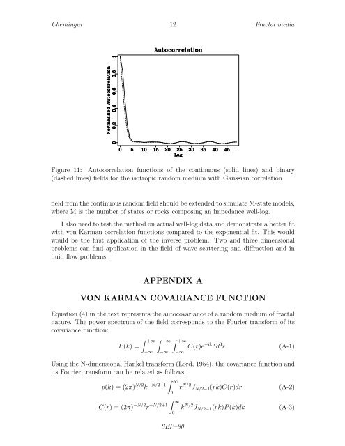
Chemingui 12 Fractal media
Figure 11: Autocorrelation functions of the continuous (solid lines) and binary
(dashed lines) fields for the isotropic random medium with Gaussian correlation
field from the continuous random field should be extended to simulate M-state models,
where M is the number of states or rocks composing an impedance well-log.
I also need to test the method on actual well-log data and demonstrate a better fit
with von Karman correlation functions compared to the exponential fit. This would
would be the first application of the inverse problem. Two and three dimensional
problems can find application in the field of wave scattering and diffraction and in
fluid flow problems.
APPENDIX A
VON KARMAN COVARIANCE FUNCTION
Equation (4) in the text represents the autocovariance of a random medium of fractal
nature. The power spectrum of the field corresponds to the Fourier transform of its
covariance function:
P (k) =
∫ +∞ ∫ +∞ ∫ +∞
−∞ −∞ −∞
C(r)e −ik·r d 3 r
(A-1)
Using the N-dimensional Hankel transform (Lord, 1954), the covariance function and
its Fourier transform can be related as follows:
∫ ∞
p(k) = (2π) N/2 k −N/2+1 r N/2 J N/2−1 (rk)C(r)dr
0
∫ ∞
C(r) = (2π) −N/2 r −N/2+1 k N/2 J N/2−1 (rk)P (k)dk
0
SEP–80
(A-2)
(A-3)