Modeling 3-D anisotropic fractal mediaa

Chemingui 4 Fractal media
1
0.9
0.8
v=1.0 −−−> Euclidian random field
v=0.0 −−−> Space filling random field
v=0.5 −−−> Exponential autocorrelation
Normalized Autocorrelation
0.7
0.6
0.5
0.4
0.3
v=1.0
v=0.5
v=0.4
v=0.3
v=0.2
0.2
v=0.1
v=0.0
0.1
0 1 2 3 4 5 6 7 8 9 10
Lag
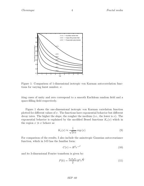
Figure 1: Comparison of 1-dimensional isotropic von Karman autocorrelation functions
for varying hurst number, ν.
iting cases of unity and zero correspond to a smooth Euclidean random field and a
space-filling field respectively.
Figure 1 shows the one-dimensional isotropic von Karman correlation function
plotted for different values of ν. The functions have exponential behavior but different
decay rates. The higher the slope, the rougher the medium (i.e., the lower is ν). The
exponential behavior is explained by the modified Bessel functions K ν (x) which in
the region x ≫ ν behave as
K ν (x) ≈ 1 √
2πx
exp (x) (9)
For comparison of the results, I also include the anisotropic Gaussian autocovariance
function, which in 3-D has the familiar form:
and its 3-dimensional Fourier transform is given by:
C(r) = H 2 e −r2 (10)
P (k) = a xa y a z
H 2 e k2 4 (11)
2
SEP–80