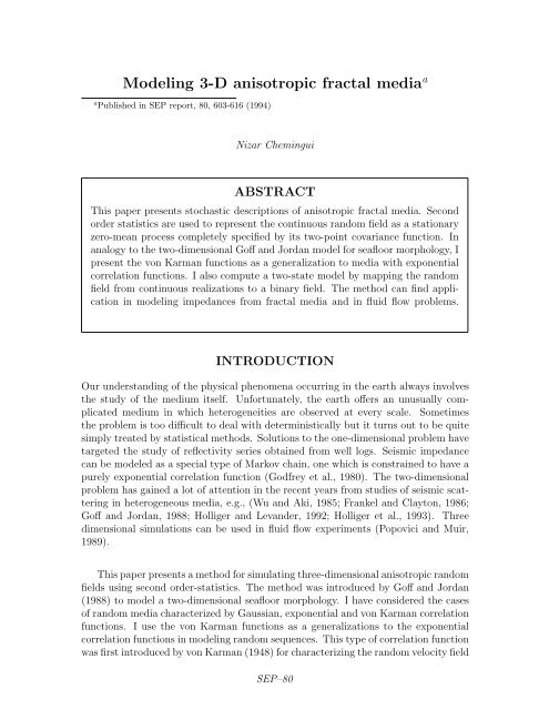
Modeling 3-D anisotropic fractal mediaa

Modeling 3-D anisotropic fractal media a 

a Published in SEP report, 80, 603-616 (1994) 

Nizar Chemingui 

ABSTRACT 

This paper presents stochastic descriptions of anisotropic fractal media. Second 

order statistics are used to represent the continuous random field as a stationary 

zero-mean process completely specified by its two-point covariance function. In 

analogy to the two-dimensional Goff and Jordan model for seafloor morphology, I 

present the von Karman functions as a generalization to media with exponential 

correlation functions. I also compute a two-state model by mapping the random 

field from continuous realizations to a binary field. The method can find application 

in modeling impedances from fractal media and in fluid flow problems. 

INTRODUCTION 

Our understanding of the physical phenomena occurring in the earth always involves 

the study of the medium itself. Unfortunately, the earth offers an unusually complicated 

medium in which heterogeneities are observed at every scale. Sometimes 

the problem is too difficult to deal with deterministically but it turns out to be quite 

simply treated by statistical methods. Solutions to the one-dimensional problem have 

targeted the study of reflectivity series obtained from well logs. Seismic impedance 

can be modeled as a special type of Markov chain, one which is constrained to have a 

purely exponential correlation function (Godfrey et al., 1980). The two-dimensional 

problem has gained a lot of attention in the recent years from studies of seismic scattering 

in heterogeneous media, e.g., (Wu and Aki, 1985; Frankel and Clayton, 1986; 

Goff and Jordan, 1988; Holliger and Levander, 1992; Holliger et al., 1993). Three 

dimensional simulations can be used in fluid flow experiments (Popovici and Muir, 

1989). 

This paper presents a method for simulating three-dimensional anisotropic random 

fields using second order-statistics. The method was introduced by Goff and Jordan 

(1988) to model a two-dimensional seafloor morphology. I have considered the cases 

of random media characterized by Gaussian, exponential and von Karman correlation 

functions. I use the von Karman functions as a generalizations to the exponential 

correlation functions in modeling random sequences. This type of correlation function 

was first introduced by von Karman (1948) for characterizing the random velocity field 

SEP–80

Chemingui 2 Fractal media 

of a turbulent medium. It has since been frequently used in the statistical literature, 

studies of turbulence problems, e.g.(Tatarski, 1961), and studies of random media such 

as wave scattering, e.g.(Chernov, 1960). The von Karman functions were identified 

specifically as belonging to the class of continuous correlation functions (Matern, 

1970). Holliger et al. (1993) used von Karman covariance functions to model binary 

fields and defined “binarization” as a mapping of all values in a continuous field to 

just two values of the new field. I have employed their technique to model two state 

models (i.e, rock/pore or sandstone/shale) from continuous realizations and test the 

increase in medium roughness through the “binarization” process. 

RANDOM FIELDS 

A stochastic model is constructed for the properties of the random medium. We first 

construct a distribution function P(x) for the properties of the medium h(x). From 

such a probability function, we can recover the statistical properties of the distribution 

(i.e., mean, variance , etc.) through its N-point statistical moments (Goff and Jordan, 

1988). 

C N (x 1 , x 2 , ..., x N ) = < h(x 1 )...h(x N ) > 

= 

∫ +∞ 

−∞ 

... 

∫ +∞ 

−∞ 

h 1 ...h N P (h 1 , ..., h N )dh 1 ...dh N (1) 

where h N = h(x N ). The key assumption of spatial homogeneity (stationarity) means 

that the N-point moments are taken to depend only on the vector joining these 

points and not on their absolute positions. These moments describe the magnitude 

and smoothness of the fluctuations of h(x). 

Second-order Statistics 

I restricted this research to the study of second-order statistics of random fields. This 

means the study of random media characterized by Gaussian distributions, where 

a Gaussian process is completely specified by its first- and second-order moments. 

Furthermore if I define the field h(x) to be a zero mean process: 

< h(x) >= 

∫ +∞ 

−∞ 

h(x)P (h(x))dh = 0 (2) 

then h(x) is fully described by its two-point moment that is its autocovariance function 

which we write as a function of the correlation function: 

C hh (r) = E[h(x)h(x + r)] = H 2 ρ hh (r) (3) 

where P (h(x)) is the probability density function of h(x), r is the lag vector, E is 

the expected value, H 2 is the variance (i.e. C hh (0)) and ρ hh is the three-dimensional 

correlation function. Equation (3) shows that the random medium can be adequately 

SEP–80


specified by its autocorrelation function. More generally, an anisotropic random field 

can be described by a monotonically decaying autocorrelation function whose rate of 

decay depends on direction. The roughness of the medium is function of the decay 

rate of the correlation. The Fourier transform of the autocorrelation is the power 

spectrum of the field (Bracewell, 1978). Three types of correlation functions were 

commonly used in the field of seismic modeling: the Gaussian, exponential and von 

Karman functions. These special functions are described by analytic expressions of 

their autocorrelations and Fourier transforms. 

Two-dimensional cases have been studied for some time(Wu and Aki, 1985; Frankel 

and Clayton, 1986; Goff and Jordan, 1988; Holliger and Levander, 1992; Holliger et al., 

1993). Within the last several years, computer capacity and speed have grown rapidly. 

It is now feasible to extend our models and simulations to the three-dimensional case. 

von Karman correlation functions 

The three-dimensional anisotropic von Karman function is given by (Goff and Jordan, 

1988): 

C(r) = 4πνH2 r ν K ν (r) 

(4) 

K ν (0) 

and its three-dimensional Fourier transform is: 

where r = 

√ 

x 2 

+ y2 

a 2 x a 2 y 

P (k) = 4πνH2 

K ν (0) 

a 2 x + a 2 y + a 2 z 

(1 + k 2 ) ν+ 3 2 

+ z2 , k = √ k 

a xa 2 2 2 x + kya 2 2 y + kza 2 2 z; a x , a y and a z are the characteris- 

z 

tic scales of the medium along the 3-dimensions and k x , k y and k z are the wavenumber 

components. K ν is the modified Bessel function of order ν, where 0.0 < ν < 1.0 is 

the Hurst number (Mandelbrot, 1983, 1985). The fractal dimension of a stochastic 

field characterized by a von Karman autocorrelation is given by: 

(5) 

D = E + 1 − ν (6) 

where E is the Euclidean dimension i.e., E = 3 for the three-dimensional problem. 

The special case of ν = 0.5 yields to the exponential covariance function that corresponds 

to a Markov process (Feller, 1971). 

whose three-dimensional Fourier transform is given by: 

C(r) = H 2 e −r (7) 

P (k) = H 2 a2 x + a 2 y + a 2 z 

(1 + k 2 ) 2 (8) 

Decreasing the Hurst number, ν, increases the roughness of the medium. The lim- 

SEP–80


1 

0.9 

0.8 

v=1.0 −−−> Euclidian random field 

v=0.0 −−−> Space filling random field 

v=0.5 −−−> Exponential autocorrelation 

Normalized Autocorrelation 

0.7 

0.6 

0.5 

0.4 

0.3 

v=1.0 

v=0.5 

v=0.4 

v=0.3 

v=0.2 

0.2 

v=0.1 

v=0.0 

0.1 

0 1 2 3 4 5 6 7 8 9 10 

Lag 

Figure 1: Comparison of 1-dimensional isotropic von Karman autocorrelation functions 

for varying hurst number, ν. 

iting cases of unity and zero correspond to a smooth Euclidean random field and a 

space-filling field respectively. 

Figure 1 shows the one-dimensional isotropic von Karman correlation function 

plotted for different values of ν. The functions have exponential behavior but different 

decay rates. The higher the slope, the rougher the medium (i.e., the lower is ν). The 

exponential behavior is explained by the modified Bessel functions K ν (x) which in 

the region x ≫ ν behave as 

K ν (x) ≈ 1 √ 

2πx 

exp (x) (9) 

For comparison of the results, I also include the anisotropic Gaussian autocovariance 

function, which in 3-D has the familiar form: 

and its 3-dimensional Fourier transform is given by: 

C(r) = H 2 e −r2 (10) 

P (k) = a xa y a z 

H 2 e k2 4 (11) 

2 

SEP–80


FORWARD MODELING 

Continuous random fields have frequently been used for statistical analyses, modeling 

perturbed media, scattering and diffraction studies, fluid flow simulations and, other 

related problems. Numerical realizations may describe the statistical character of 

random models at all scales. 

Numerical Implementation 

The generation of synthetic random media is done in the wave number domain. First, 

we compute the power spectrum of the field, i.e, the Fourier spectrum of the autocorrelation 

function. Then we compute the Fourier spectrum by multiplying the square 

root of the power spectrum by a random phase factor e 2πη where η is a uniform deviate 

that lies in the interval [0,1). In a final step we apply an inverse fast Fourier 

transform to obtain the spatial domain representation of the random medium. The 

numerical implementation of the method is very straightforward, although special 

care is required to handle D.C. and Nyquist wavenumbers. 

Algorithms are similar for the one-, two- and three-dimensional problem although if 

we do not care about computer expenses, 1- and 2-D random sequences can be simply 

extracted as arrays or sections from 3-D simulations. 

Figure 2: Synthetic random field with anisotropic Gaussian autocorrelation function; 

a x = 15, a y = 25, a z = 35. 

SEP–80


Figure 3: Synthetic random field with anisotropic exponential autocorrelation function; 

a x = 15, a y = 25, a z = 35. 

Figure 4: Synthetic random field with anisotropic von Karman autocorrelation function; 

a x = 15, a y = 25, a z = 35. 

SEP–80


Modeling 3-D random media 

I show three different realizations of an anisotropic model with different aspect ratios 

along the three coordinate axes. The model is a 64 points cube with characteristic 

scales a x = 15, a y = 25, and a z = 35. The media are characterized by Gaussian, 

exponential, and van karman autocorrelation functions, respectively. We notice the 

increase in model roughness as we move from the Gaussian medium to the exponential 

field (i.e, ν = .5) and then to the von Karman field with ν = .2. 

In the physical world, these fields may represent media at different scales varying 

from the microscopic to the megascopic. 

Modeling seismic impedances 

Seismic impedances have frequently been modeled as a Markov process. Godfrey 

et. al. (1980) modeled impedance as a special type of Markov chain, one that is 

constrained to have a purely exponential correlation function. They tested their 

method on three actual logs and compared the autocorrelation function to a best fit 

exponential curve. Apart from a small geologic noise component at the origin, their 

results showed excellent agreement between the theoretical exponential and the actual 

autocorrelation on two of the well logs they considered. For large lags, the actual 

correlation function had exponential behavior similar to that of the theoretical curve, 

but all data points fell below the synthetic curve showing a faster decay rate. The 

behavior of the autocorrelation could very well be interpreted as related to a rougher 

distribution than that predicted by the exponential correlation. A von Karman correlation 

function with a Hurst number smaller than 0.5 would have given a better fit 

to the autocorrelation of the impedance series. The autocorrelation of the impedance 

function provides information on the depositional pattern in the sedimentary column 

i.e, cyclic or transitional (O’Doherty and Anstey, 1971). 

Figure 5 shows a comparison of one-dimensional random sequences that simulate 

synthetic impedances with von Karman correlation functions of varying fractal dimensions 

(i.e., Hurst number ν). Again the smaller the value of ν, the rougher the 

sequence. The impedance with exponential correlation seems smooth compared to 

the ones generated from autocorrelation functions with values of ν lower than 0.5. 

GENERATING TWO-STATE MODELS 

In the geophysical world we often deal with heterogeneous media whose inhomogeneities 

are caused by the presence of two different types of material with different 

mechanical properties. A typical example is the case of a stratified formation of shale 

embedded in sandstone. In fluid flow and reservoir engineering problems, the rock 

samples are generally composed of a matrix and pore space. Continuously random 

fields are therefore inadequate to describe randomness in similar settings. I seek to 

SEP–80


v=1.0 

v=0.5 

v=0.4 

v=0.3 

v=0.2 

v=0.1 

v=0.0 

Figure 5: Synthetic random sequences simulating acoustic impedances with von Karman 

autocorrelation for varying Hurst number ν. 

describe a random field in which the medium can be represented as a two-state model. 

This new field is called a binary field and the process of deriving the binary field from 

the continuous field is called “binarization” (Holliger et al., 1993). The problem is to 

relate the statistics of the binary field to those of the continuous field. Holliger et al. 

(1993) gave a brief description of their mapped two-dimensional binary field which I 

apply in a straightforward generalization to the three-dimensional problem. 

To illustrate the effects of “binarizing” a continuous field, let’s consider two examples 

of random fields with Gaussian and exponential autocorrelation functions, respectively. 

In the first example I simulate a randomly-stratified medium. The second 

example is a realization of a random medium with statistically isotropic homogeneous 

inclusions. I like to analyze the change in the medium properties by comparing the 

autocorrelation function of the distribution before and after “binarization”. For better 

observation, I limit the analysis to the study of the correlation function along one 

axis, i.e, in the x-direction. 

Figure ?? shows the averaged 1-D correlation function along the x-axis for the 

randomly layered medium. The solid curve displays the autocorrelation of the continuous 

field; the dashed one represents the autocorrelation of the “binary” field. The 

two functions are noticeably different from one another; the slope near the origin is 

greatly increased after “binarization” indicating a rougher distribution compared to 

the continuous case. Figure ?? shows the same observations for the isotropic random 

field with Gaussian autocorrelation; again the roughness of the field has increased as 

SEP–80


indicated by the steepening in the slope of the autocorrelation. 

Figure 6: Synthetic continuous random field with apparent layering and Gaussian 

autocorrelation; a x = 5, a y = 80, a z = 80. 

CONCLUSIONS 

In this initial study I have tackled the forward problem for modeling anisotropic 

fractal media using second-order statistics. The method has close analogy with the 

two-dimensional Goff and Jordan model for seafloor morphology. The generation of 

synthetic models is done in the Fourier domain and the algorithms are similar for the 

one- two- and three-dimensional problems. The von Karman functions are presented 

as a generalization of the exponential correlation function associated with the Markov 

process in modeling seismic impedances. The von Karman functions can be used for 

better description of statistic lithology of stratigraphic columns and understanding 

their depositional pattern. I have also computed a two-state model (i.e., rock/pore 

or sandstone/shale) by mapping the random field from continuous realizations into 

a binary field. Comparisons of the autocorrelation functions of the continuous and 

binary fields show that the fractal dimension (i.e, the roughness of the medium) 

increases through the “binarization” process. 

FUTURE WORK 

Future goals of this effort will be to formulate the inverse problem for estimating 

the characteristic parameters of the anisotropic fractal medium, i.e, aspect ratios of 

anisotropy, and Hausdorff (fractal) dimension. The technique of deriving the binary 

SEP–80


Figure 7: Synthetic binary field derived from the continuous realization of a layered 

random field with Gaussian autocorrelation. 

Figure 8: Synthetic continuous random field with isotropic Gaussian autocorrelation 

function; a x = 15, a y = 15, a z = 15. 

SEP–80


Figure 9: Synthetic binary field derived from the continuous realization of a random 

field with Gaussian autocorrelation. 

Figure 10: Autocorrelation functions of the continuous (solid lines) and binary 

(dashed lines) fields for the layered random medium with exponential correlation. 

SEP–80


Figure 11: Autocorrelation functions of the continuous (solid lines) and binary 

(dashed lines) fields for the isotropic random medium with Gaussian correlation 

field from the continuous random field should be extended to simulate M-state models, 

where M is the number of states or rocks composing an impedance well-log. 

I also need to test the method on actual well-log data and demonstrate a better fit 

with von Karman correlation functions compared to the exponential fit. This would 

would be the first application of the inverse problem. Two and three dimensional 

problems can find application in the field of wave scattering and diffraction and in 

fluid flow problems. 

APPENDIX A 

VON KARMAN COVARIANCE FUNCTION 

Equation (4) in the text represents the autocovariance of a random medium of fractal 

nature. The power spectrum of the field corresponds to the Fourier transform of its 

covariance function: 

P (k) = 

∫ +∞ ∫ +∞ ∫ +∞ 

−∞ −∞ −∞ 

C(r)e −ik·r d 3 r 

(A-1) 

Using the N-dimensional Hankel transform (Lord, 1954), the covariance function and 

its Fourier transform can be related as follows: 

∫ ∞ 

p(k) = (2π) N/2 k −N/2+1 r N/2 J N/2−1 (rk)C(r)dr 

0 

∫ ∞ 

C(r) = (2π) −N/2 r −N/2+1 k N/2 J N/2−1 (rk)P (k)dk 

0 

SEP–80 

(A-2) 

(A-3)


where J N/2−1 is the Bessel function of order N/2 − 1. 

The covariance C(r) in (3) is specified in terms of the function: 

G ν (r) = r ν K ν (r) 0 ≤ r < ∞ ν ∈ [0, 1] (A-4) 

whose Hankel transform pair has been derived by Lord (1954): 

P (k) = 

where Γ is the gamma function defined as: 

Γ(ν + N/2) 

2 1−N−ν π N /2 (1 + k2 ) −ν−N/2 (A-5) 

Γ(z) = 

∫ ∞ 

0 

t z−1 e −t dt 

(A-6) 

Finally if we normalize G ν (r) by G ν (0) as in Goff and Jordan (1988), we obtain, 

for the three-dimensional case, the power spectrum of the field whose covariance is 

defined by (4): 

P (k) = 4πνH 2 (1 + k 2 ) (−ν−3/2) 

(A-7) 

REFERENCES 

Bracewell, R., 1978, The Fourier transform and its application: McGraw-Hill, New 

York. 

Chernov, L. A., 1960, Wave propagation in a random medium: McGraw-Hill, New 

York. 

Feller, W., 1971, An introduction to probability theory and its applications: Vol. 2: 

John Wiley, New York. 

Frankel, A., and R. W. Clayton, 1986, Finite difference simulations of seismic scattering: 

Implications for the propagation of short-period seismic waves in the crust and 

models of crustal heterogeneity: Journal of Geophysical Research, 91, 6465–6489. 

Godfrey, R., F. Muir, and F. Rocca, 1980, Modeling seismic impedance with Markov 

chains: Geophysics, 45, 1351–1372. 

Goff, J. A., and T. H. Jordan, 1988, Stochastic modeling of seafloor morphology: 

Inversion of sea beam data for second-order statistics: Journal of Geophysical Research, 

93, 13,589–13,608. 

Holliger, K., and A. R. Levander, 1992, A stochastic view of lower crustal fabric based 

on evidence from the Ivrea zone: Geophysical Research Letters, 19, 1153–1156. 

Holliger, K., A. R. Levander, and J. A. Goff, 1993, Stochastic modeling of the reflective 

lower crust: petrophysical and geological evidence from the Ivrea zone 

(Northern Italy): Journal of Geophysical Research, 98, 11967–11980. 

Lord, R. D., 1954, The use of the Hankel transform in statistics: I. General theory 

and examples: Biometrika, 41, 44–55. 

Mandelbrot, B. B., 1983, The fractal geometry of nature: W. H. Freeman, New York. 

——–, 1985, Self-affine fractals and and fractal dimension: Phys. Scrip., 32, 257–260. 

Matern, B., 1970, Spatial variation: Medd. Skogsforskn Inst., 49(5), 1–144. 

SEP–80


O’Doherty, R. F., and N. A. Anstey, 1971, Reflections on amplitudes: Geophysical 

Prospecting, 19, 430–458. 

Popovici, M., and F. Muir, 1989, Modeling anisotropic porous rocks, in SEP-60: 

Stanford Exploration Project, 295–302. 

Tatarski, V. I., 1961, Wave propagation in a turbulent medium: McGraw-Hill, New 

York. 

Wu, R. S., and K. Aki, 1985, The fractal nature of inhomogeneities in the lithosphere 

evidenced from seismic wave scattering: Pure and Applied Geophysics, 123, 805– 

818. 

SEP–80

Modeling 3-D anisotropic fractal mediaa

You also want an ePaper? Increase the reach of your titles

Delete template?

Save as template?