Numerical Advection Schemes in Two Dimensions
Numerical Advection Schemes in Two Dimensions
Numerical Advection Schemes in Two Dimensions

Create successful ePaper yourself
Turn your PDF publications into a flip-book with our unique Google optimized e-Paper software.
3.2 Directional splitt<strong>in</strong>g 3 ADVECTING IN TWO DIMENSIONS<br />
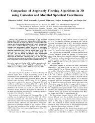
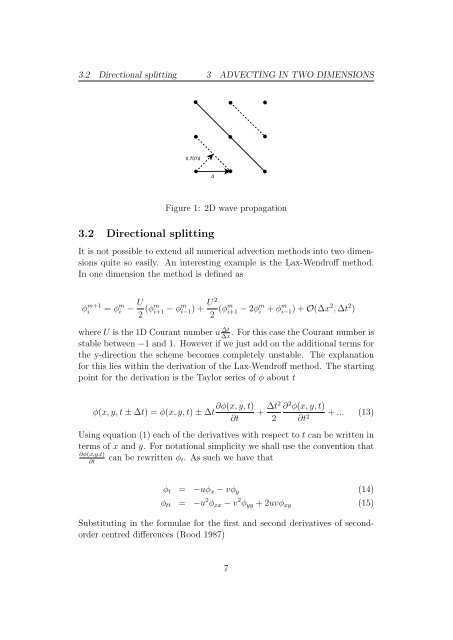
0.707d<br />
d<br />
3.2 Directional splitt<strong>in</strong>g<br />
Figure 1: 2D wave propagation<br />
It is not possible to extend all numerical advection methods <strong>in</strong>to two dimensions<br />
quite so easily. An <strong>in</strong>terest<strong>in</strong>g example is the Lax-Wendroff method.<br />
In one dimension the method is def<strong>in</strong>ed as<br />
ϕ m+1<br />
i = ϕ m i − U 2 (ϕm i+1 − ϕ m i−1) + U 2<br />
2 (ϕm i+1 − 2ϕ m i + ϕ m i−1) + O(∆x 2 , ∆t 2 )<br />
where U is the 1D Courant number u ∆t . For this case the Courant number is<br />
∆x<br />
stable between −1 and 1. However if we just add on the additional terms for<br />
the y-direction the scheme becomes completely unstable. The explanation<br />
for this lies with<strong>in</strong> the derivation of the Lax-Wendroff method. The start<strong>in</strong>g<br />
po<strong>in</strong>t for the derivation is the Taylor series of ϕ about t<br />
∂ϕ(x, y, t)<br />
ϕ(x, y, t ± ∆t) = ϕ(x, y, t) ± ∆t + ∆t2 ∂ 2 ϕ(x, y, t)<br />
+ ... (13)<br />
∂t 2 ∂t 2<br />
Us<strong>in</strong>g equation (1) each of the derivatives with respect to t can be written <strong>in</strong><br />
terms of x and y. For notational simplicity we shall use the convention that<br />
can be rewritten ϕ t . As such we have that<br />
∂ϕ(x,y,t)<br />
∂t<br />
ϕ t = −uϕ x − vϕ y (14)<br />
ϕ tt = −u 2 ϕ xx − v 2 ϕ yy + 2uvϕ xy (15)<br />
Substitut<strong>in</strong>g <strong>in</strong> the formulae for the first and second derivatives of secondorder<br />
centred differences (Rood 1987)<br />
7