LIGO-P030036-00-R - Ligo - Caltech
LIGO-P030036-00-R - Ligo - Caltech
LIGO-P030036-00-R - Ligo - Caltech

You also want an ePaper? Increase the reach of your titles
YUMPU automatically turns print PDFs into web optimized ePapers that Google loves.
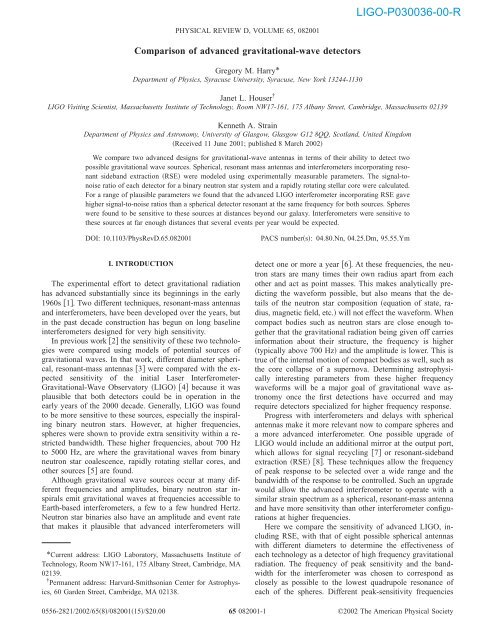
<strong>LIGO</strong>-<strong>P03<strong>00</strong>36</strong>-<strong>00</strong>-R<br />
PHYSICAL REVIEW D, VOLUME 65, 082<strong>00</strong>1<br />
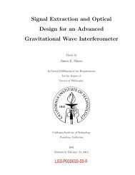
Comparison of advanced gravitational-wave detectors<br />
Gregory M. Harry*<br />
Department of Physics, Syracuse University, Syracuse, New York 13244-1130<br />
Janet L. Houser †<br />
<strong>LIGO</strong> Visiting Scientist, Massachusetts Institute of Technology, Room NW17-161, 175 Albany Street, Cambridge, Massachusetts 02139<br />
Kenneth A. Strain<br />
Department of Physics and Astronomy, University of Glasgow, Glasgow G12 8QQ, Scotland, United Kingdom<br />
Received 11 June 2<strong>00</strong>1; published 8 March 2<strong>00</strong>2<br />
We compare two advanced designs for gravitational-wave antennas in terms of their ability to detect two<br />
possible gravitational wave sources. Spherical, resonant mass antennas and interferometers incorporating resonant<br />
sideband extraction RSE were modeled using experimentally measurable parameters. The signal-tonoise<br />
ratio of each detector for a binary neutron star system and a rapidly rotating stellar core were calculated.<br />
For a range of plausible parameters we found that the advanced <strong>LIGO</strong> interferometer incorporating RSE gave<br />
higher signal-to-noise ratios than a spherical detector resonant at the same frequency for both sources. Spheres<br />
were found to be sensitive to these sources at distances beyond our galaxy. Interferometers were sensitive to<br />
these sources at far enough distances that several events per year would be expected.<br />
DOI: 10.1103/PhysRevD.65.082<strong>00</strong>1<br />
PACS numbers: 04.80.Nn, 04.25.Dm, 95.55.Ym<br />
I. INTRODUCTION<br />
The experimental effort to detect gravitational radiation<br />
has advanced substantially since its beginnings in the early<br />
1960s 1. Two different techniques, resonant-mass antennas<br />
and interferometers, have been developed over the years, but<br />
in the past decade construction has begun on long baseline<br />
interferometers designed for very high sensitivity.<br />
In previous work 2 the sensitivity of these two technologies<br />
were compared using models of potential sources of<br />
gravitational waves. In that work, different diameter spherical,<br />
resonant-mass antennas 3 were compared with the expected<br />
sensitivity of the initial Laser Interferometer-<br />
Gravitational-Wave Observatory <strong>LIGO</strong> 4 because it was<br />
plausible that both detectors could be in operation in the<br />
early years of the 2<strong>00</strong>0 decade. Generally, <strong>LIGO</strong> was found<br />
to be more sensitive to these sources, especially the inspiraling<br />
binary neutron stars. However, at higher frequencies,<br />
spheres were shown to provide extra sensitivity within a restricted<br />
bandwidth. These higher frequencies, about 7<strong>00</strong> Hz<br />
to 5<strong>00</strong>0 Hz, are where the gravitational waves from binary<br />
neutron star coalescence, rapidly rotating stellar cores, and<br />
other sources 5 are found.<br />
Although gravitational wave sources occur at many different<br />
frequencies and amplitudes, binary neutron star inspirals<br />
emit gravitational waves at frequencies accessible to<br />
Earth-based interferometers, a few to a few hundred Hertz.<br />
Neutron star binaries also have an amplitude and event rate<br />
that makes it plausible that advanced interferometers will<br />
*Current address: <strong>LIGO</strong> Laboratory, Massachusetts Institute of<br />
Technology, Room NW17-161, 175 Albany Street, Cambridge, MA<br />
02139.<br />
† Permanent address: Harvard-Smithsonian Center for Astrophysics,<br />
60 Garden Street, Cambridge, MA 02138.<br />
detect one or more a year 6. At these frequencies, the neutron<br />
stars are many times their own radius apart from each<br />
other and act as point masses. This makes analytically predicting<br />
the waveform possible, but also means that the details<br />
of the neutron star composition equation of state, radius,<br />
magnetic field, etc. will not effect the waveform. When<br />
compact bodies such as neutron stars are close enough together<br />
that the gravitational radiation being given off carries<br />
information about their structure, the frequency is higher<br />
typically above 7<strong>00</strong> Hz and the amplitude is lower. This is<br />
true of the internal motion of compact bodies as well, such as<br />
the core collapse of a supernova. Determining astrophysically<br />
interesting parameters from these higher frequency<br />
waveforms will be a major goal of gravitational wave astronomy<br />
once the first detections have occurred and may<br />
require detectors specialized for higher frequency response.<br />
Progress with interferometers and delays with spherical<br />
antennas make it more relevant now to compare spheres and<br />
a more advanced interferometer. One possible upgrade of<br />
<strong>LIGO</strong> would include an additional mirror at the output port,<br />
which allows for signal recycling 7 or resonant-sideband<br />
extraction RSE 8. These techniques allow the frequency<br />
of peak response to be selected over a wide range and the<br />
bandwidth of the response to be controlled. Such an upgrade<br />
would allow the advanced interferometer to operate with a<br />
similar strain spectrum as a spherical, resonant-mass antenna<br />
and have more sensitivity than other interferometer configurations<br />
at higher frequencies.<br />
Here we compare the sensitivity of advanced <strong>LIGO</strong>, including<br />
RSE, with that of eight possible spherical antennas<br />
with different diameters to determine the effectiveness of<br />
each technology as a detector of high frequency gravitational<br />
radiation. The frequency of peak sensitivity and the bandwidth<br />
for the interferometer was chosen to correspond as<br />
closely as possible to the lowest quadrupole resonance of<br />
each of the spheres. Different peak-sensitivity frequencies<br />
0556-2821/2<strong>00</strong>2/658/082<strong>00</strong>115/$20.<strong>00</strong><br />
65 082<strong>00</strong>1-1<br />
©2<strong>00</strong>2 The American Physical Society
HARRY, HOUSER, AND STRAIN PHYSICAL REVIEW D 65 082<strong>00</strong>1<br />
for the interferometer are obtained by varying the position of<br />
the signal-extraction mirror by a fraction of the wavelength<br />
of the laser light. The fractional bandwidth of a sphere is<br />
determined by the choice of transducer, and is typically below<br />
20%. To reproduce this narrow bandwidth, the transmittance<br />
of the interferometer’s signal-extraction mirror has<br />
been chosen to be relatively low. Once the interferometer has<br />
been matched to a given sphere, the sensitivity of the sphere<br />
and interferometer to different, high frequency, sources can<br />
be compared.<br />
The signal-to-noise ratio for both the spheres and the interferometer<br />
was computed using the numerically simulated<br />
relativistic waveforms of two different gravitational wave<br />
burst sources: 1 the inspiral and eventual coalescence of a<br />
binary neutron star system, and 2 a rapidly rotating stellar<br />
core undergoing a dynamical instability 9,10. Both of these<br />
sources are predicted to have high enough event rates that<br />
they could be detected by interferometers within the next ten<br />
years 4–6,11,12<br />
There are many other sources of gravitational waves that<br />
could provide interesting physical and/or astrophysical information.<br />
The stochastic background of gravitational radiation<br />
depends on conditions at the earliest times in the universe<br />
13 and their detection would shed new light on cosmology.<br />
Searches for scalar radiation would allow for tests of gravity<br />
beyond the prediction of general relativity. Both interferometers<br />
and spheres may play a role in these experiments, but<br />
we did not consider these sources in this work.<br />
II. METHOD<br />
FIG. 1. Schematic drawing of a spherical, resonant mass, gravitational<br />
wave detector with a three-mode transducer attached. The<br />
sphere mass, m s , is connected to mechanical ground, here the center<br />
of mass of the sphere. The gravitational wave acts as a force, F,<br />
between the sphere mass and ground. Each of the complex spring<br />
constants, k s , k 1 , and k 2 , includes dissipation which gives rise to<br />
thermal noise. The transducer mass is next to a superconducting<br />
pick up coil which stores a persistent current. This current is<br />
shunted to the input coil of the SQUID in proportion to the motion<br />
of the mass. The SQUID amplifies the signal and also serves as a<br />
source of wideband noise.<br />
The spherical antennas were modeled using the same<br />
method as described in the previous paper 2. A conceptual<br />
error in the code developed for the previous paper has been<br />
corrected here. This error effects the form of the y( f ) matrix<br />
and changed the SNRs calculated by a few percent. The<br />
signal-to-noise ratio density was calculated for each sphere<br />
using the method of Price 14 as extended by Stevenson<br />
15. This involved calculating the signal-to-noise ratio density<br />
from the strain spectrum of each sphere. The parameters<br />
that entered the strain spectrum were chosen based, as much<br />
as possible, on optimistic extrapolations from values demonstrated<br />
in operating detectors.<br />
Eight aluminum spheres were modeled with diameters of<br />
3.25 m, 2.75 m, 2.35 m, 2.<strong>00</strong> m, 1.70 m, 1.45 m, 1.25 m, and<br />
1.05 m. The 3.25 m sphere weighs 50 tons and is the largest<br />
solid sphere which can reasonably be manufactured and<br />
transported. It may be possible to get larger radii spheres,<br />
and hence lower resonance frequencies, by building hollow<br />
spheres 16 but we did not consider these detectors. A lower<br />
frequency, hollow sphere will have advantages with lower<br />
frequency sources, especially the inspiral phase of the binary<br />
neutron star signal, but not with the higher frequency sources<br />
we considered here. Each sphere was modeled as having six,<br />
three-mode inductive transducers arranged in the TIGA geometry<br />
3 which allows for omnidirectional sensitivity. The<br />
masses of the intermediate mass and the final transducer<br />
mass see Fig. 1 were chosen to give a fractional bandwidth<br />
as large a possible for each sphere. The transducer was modeled<br />
as having a dual, superconducting quantum interference<br />
device SQUID as the first stage amplifier. SQUID amplifiers<br />
are currently in use on bar detectors 17,18. A threemode<br />
transducer is being developed for use on the Allegro<br />
antenna 19 and one has been successfully demonstrated on<br />
a test antenna 20.<br />
The limiting noise in a spherical resonant mass detector<br />
comes from two sources; amplifier noise and thermal noise.<br />
The amplifier noise, which comes primarily from the sensing<br />
SQUID, can be separated into additive velocity noise and<br />
force noise. The additive velocity noise can be written as 2<br />
S u f N n 2 f 0 /r n ,<br />
where N n is the noise number of the SQUID, is Planck’s<br />
constant, f 0 is the resonant frequency of the sphere, and r n is<br />
the noise resistance of the transducer. We assumed that the<br />
SQUID had quantum-limited noise, and hence a noise number<br />
equal to one. A quantum-limited SQUID suitable for use<br />
in a gravitational wave transducer has not yet been demonstrated,<br />
although the quantum limit has been reached in<br />
SQUIDs with low input impedance 21. A noise number of<br />
24 has been reached at 1<strong>00</strong> mK in a suitable SQUID when<br />
cooled on its own 22. This noise, however, was found to<br />
increase significantly when placed in a transducer 23.<br />
There are recent indications that commercial SQUIDs can be<br />
modified so that they have a noise number near 2<strong>00</strong> 24.<br />
This has yet to be completely verified in an operating transducer,<br />
however.<br />
The noise resistance was calculated from<br />
r n A coil /4 f 0 ,<br />
where is an experimentally determined spring constant<br />
density given in Table I and A coil „(d c /2) 2 … is the area of<br />
the pick-up coils. The noise resistance limits the bandwidth<br />
1<br />
2<br />
082<strong>00</strong>1-2
COMPARISON OF ADVANCED GRAVITATIONAL-WAVE ... PHYSICAL REVIEW D 65 082<strong>00</strong>1<br />
TABLE I. Parameters used in model of spherical, resonant mass, gravitational wave antennas.<br />
Parameter Name Value Source<br />
Q s Sphere quality factor, Al 4010 6 27<br />
Q 1 Intermediate mass quality factor, Al 4010 6 27<br />
Q 2 Transducer mass quality factor, Nb 4010 6 28,29<br />
T Temperature 50 mK 26<br />
T n SQUID noise number 1 23,24<br />
d c Sensing coil diameter 9 cm 2,30<br />
Electrical spring constant per area 3.7810 8 N/m 3 2<br />
m s /m 1 Mass ratio 1<strong>00</strong> 2<br />
m 1 /m 2 Mass ratio 1<strong>00</strong> 2<br />
of a sphere with three-mode transducers when the masses<br />
are properly chosen according to 14<br />
BW „r n /2 f 0 m s … 1/5 ,<br />
where m s is the effective mass of the sphere for impedance<br />
calculations. This effective mass is given by 15,25<br />
m s 5/6m p ,<br />
3<br />
4<br />
y 22 f 2 fic 2 „14 2 f 2 c s m 1 m 2 m s <br />
4 2 f 2 c 1 m 1 m 2 4 2 f 2 c s m s 1…/<br />
„14 2 f 2 c 2 m 2 4 2 f 2 c s m 1 m 2 m s<br />
4 2 f 2 c 2 m 1 m 2 4 2 f 2 c 2 m s m s <br />
4 2 f 2 c 1 4 2 f 2 c s m s 1<br />
m 2 m 1 4 2 f 2 c 2 m 2 1….<br />
6<br />
where 0.301 25, m p is the physical mass of the sphere,<br />
and the factor 5/6 is appropriate for six transducers in the<br />
TIGA arrangement 15. The amplifier velocity noise is<br />
shown in Fig. 2 graphed as a strain spectrum.<br />
The force noise from the SQUID is ultimately detected as<br />
motion, and therefore must be converted by the mechanical<br />
transfer function of the antenna. The output noise can be<br />
written 2<br />
S f , out f N n 2 f 0 r n y 22 f 2 ,<br />
where the admittance matrix element y 22 ( f ) for a sphere<br />
with three-mode transducers can be written<br />
5<br />
In the above, c 1 is the reciprocal spring constant k 1 for the<br />
spring separating the sphere from the intermediate mass of<br />
the transducer, c 2 is the reciprocal spring constant k 2 for the<br />
spring separating the intermediate mass from the transducer<br />
mass, c s is the reciprocal spring constant k s of the effective<br />
spring separating the effective mass of the sphere from mechanical<br />
ground, m 1 is the mass of the intermediate mass of<br />
the transducer, m 2 is the mass of the transducer mass, and m s<br />
is the effective mass of the sphere for the lowest quadrupole<br />
mode. The masses and springs in the transducer are shown in<br />
Fig. 1. The spring constants can be written for each stage in<br />
the transducer ( j1,2, or s)<br />
k j 2 f 0 2 m j i2 f 2 f 0 m j /Q j ,<br />
7<br />
where Q j is the quality factor of the appropriate stage of the<br />
transducer and sphere. The Q’s depend on composition, temperature,<br />
and the connections between the masses and<br />
springs. The amplifier force noise is shown in Fig. 2 graphed<br />
as a strain spectrum.<br />
The thermal noise of the sphere can be written 2<br />
FIG. 2. Strain spectra for a 3.25 m diameter spherical, resonant<br />
mass antenna including the components of the noise. The dashed<br />
line shows the thermal noise at 50 mK, the dotted line shows the<br />
velocity forward action amplifier noise from the quantum limited<br />
SQUID, and the dashed-dotted line shows the force back-action<br />
amplifier noise from the same SQUID. The solid line is the total<br />
noise from the spherical antenna.<br />
S sph,therm 2k B T R„y 22 f …,<br />
where T is the physical temperature of the sphere. We modeled<br />
the antenna as having a T of 50 mK, although 95 mK is<br />
the lowest a bar has been cooled at equilibrium 26. The<br />
term R„y 22 ( f )… depends on the Q’s, with higher Q’s resulting<br />
in lower thermal noise. The sphere and intermediate mass<br />
8<br />
082<strong>00</strong>1-3
HARRY, HOUSER, AND STRAIN PHYSICAL REVIEW D 65 082<strong>00</strong>1<br />
were modeled in aluminum and the transducer mass was<br />
modeled in niobium. Each of the mechanical Q’s was modeled<br />
as 4010 6 27–29. Depending on the design of the<br />
transducer, the final Q can be degraded by the addition of<br />
loss from electrical coupling to the SQUID circuit 30. The<br />
sphere’s thermal noise is shown in Fig. 2 graphed as a strain<br />
spectrum.<br />
All of the noise sources for the sphere were then combined<br />
to determine the total noise<br />
S tot f S u f S f , out f S sph,therm .<br />
9<br />
This total noise is shown, along with each component, in Fig.<br />
2 graphed as a strain spectrum.<br />
The gravitational wave signal is applied as force on the<br />
spherical antenna, but is read out as velocity of the transducer<br />
mass. Thus, before a signal can be compared to these<br />
noise sources, the gravitational strain must be converted to a<br />
force and be passed through the admittance matrix of the<br />
sphere-transducer system. The comparable signal can be<br />
written 2<br />
f Y 5/2 m s<br />
f 0 3 3/2 f 2 y 21 f h f 2 , 10<br />
where Y is Young’s modulus for the sphere material, is the<br />
density of the sphere material, is the reduced cross section<br />
of the sphere and equals 0.215 for the lowest quadrupole<br />
mode 25, h( f ) is the frequency-domain amplitude of the<br />
gravitational wave, and the admittance matrix element y 21 ( f )<br />
can be written<br />
y 21 f 8 3 f 3 ic 2 c s m 2 /„14 2 f 2 c 2 m 2 4 2 f 2 c s m 1<br />
m 2 m s 4 2 f 2 c 2 m 1 m 2 4 2 f 2 c 2 m 2 m s …<br />
4 2 f 2 c 1 14 2 f 2 c s m s „m 2 m 1 1<br />
4 2 f 2 c 2 m 2 ….<br />
11<br />
Table I shows all the parameters used in the sphere model.<br />
The interferometer was modeled using a slightly modified<br />
version of the BENCH program 31. BENCH version 1.11 was<br />
the basis of our model, but it was ported to MATHEMATICA<br />
from MATLAB and a few noise formulas were updated. The<br />
factors of two errors in the thermal noise in BENCH 1.11 were<br />
fixed. The equations presented below are the ones used in<br />
our model.<br />
The noise in the interferometer is dominated by three<br />
types of noise; seismic, thermal, and optical readout noise.<br />
Each noise source was modeled using parameters from the<br />
advanced <strong>LIGO</strong> white paper 32, which is scheduled to be<br />
implemented in 2<strong>00</strong>5. The corresponding advanced interferometer<br />
is scheduled to begin taking data in 2<strong>00</strong>7. A schematic<br />
drawing of <strong>LIGO</strong> with RSE is shown in Fig. 3<br />
Seismic noise is expected to dominate the advanced <strong>LIGO</strong><br />
noise budget at low frequencies. To reduce the effect of seismic<br />
noise, each element of the interferometer will be supported<br />
by a four-stage suspension which in turn is supported<br />
from a vibration isolation stack. This vibration isolation will<br />
consist of two stages of six-degree of freedom isolation. It<br />
FIG. 3. Schematic drawing of an interferometric gravitational<br />
wave detector equipped for resonant sideband extraction. The laser<br />
creates a light beam which is sent through the power recycling<br />
mirror into two arms of a Michelson interferometer. The signal exits<br />
at the output port through the signal recycling mirror, which forms<br />
an additional Fabry-Pérot cavity with the Michelson interferometer.<br />
Finally, the signal is detected past the signal recycling mirror with a<br />
photodiode.<br />
will use a combination of active and passive isolation with<br />
an external hydraulic actuation stage. The isolation was designed<br />
to make seismic noise negligible compared to other<br />
noise sources above some f seismic , expected to be 10 Hz. In<br />
the model, seismic noise was made extremely high below 10<br />
Hz and vanishingly small above this frequency.<br />
Thermal noise will be the dominant noise source in advanced<br />
<strong>LIGO</strong> in the intermediate frequency band above 10<br />
Hz. This noise can be divided into two types; thermal noise<br />
from the internal degrees of freedom of the interferometer<br />
mirrors, and thermal noise from the suspension that supports<br />
the mirrors. The mirrors are planned to be made of m-axis<br />
sapphire, 28 cm in diameter and 30 kg in mass. Sapphire has<br />
been found to have much lower internal friction than fused<br />
silica 33,34, which is used in initial <strong>LIGO</strong>. However, sapphire<br />
suffers from much higher thermoelastic damping than<br />
silica 35.<br />
The internal mode thermal noise from the sapphire mirror<br />
comes from structural damping and thermoelastic damping.<br />
The noise from structural damping can be found from the<br />
loss angle by<br />
S str f 1 16k B T<br />
C<br />
L 2 f 1 C 2 ,<br />
12<br />
where k B is Boltzmann’s constant, T is the temperature, f is<br />
the frequency, and L is the interferometer arm length. The<br />
constants C 1 and C 2 are the overlap between the normal<br />
modes of the mirrors and the gaussian-profile laser, which<br />
has a width w 1 at the input mirror and w 2 at the end mirror.<br />
They are found from 36,37<br />
082<strong>00</strong>1-4
COMPARISON OF ADVANCED GRAVITATIONAL-WAVE ... PHYSICAL REVIEW D 65 082<strong>00</strong>1<br />
C j 12 N<br />
<br />
rY i1<br />
exp„ iw j /2r 2 … 1exp4 i h/r4 i h/r exp2 i h/r<br />
i J 0 i 2 1exp2 i h/r 2 4 i h/r 2 exp2 i h/r<br />
<br />
r2<br />
6h 3 Y<br />
h 4 /r 4 12h 2 <br />
i1<br />
N<br />
exp„i w j /2r 2 /2…<br />
i 2 J 0 i <br />
N<br />
721 i1<br />
<br />
exp„i w j /2r 2 /2…<br />
i 2 J 0 i <br />
2<br />
,<br />
13<br />
where is the Poisson ratio of the mirror material, Y is it<br />
Young’s modulus, r is the radius of the mirror, l is the thickness<br />
of the mirror, w is the Gaussian beam width of the laser<br />
at the mirror, i are the zeros of the first order Bessel function<br />
J 1 , and J 0 is the zeroth order Bessel function. The value<br />
of used is the lowest value measured for a piece of sapphire<br />
33. The thermal noise effects of making a sapphire<br />
piece into a mirror are under study, but the polishing and<br />
especially coating of the mirror are expected to cause some<br />
excess loss 38,39.<br />
Thermoelastic damping also contributes to thermal noise<br />
from the mirrors. It is found, in the limit of large mirror<br />
diameter, from 35<br />
S th f 1T<br />
fLC V <br />
<br />
2 16k B<br />
1/w 1 3 1/w 3 2 , 14<br />
where is the thermal expansion coefficient, C V is the heat<br />
capacity at constant volume, is the density, and is the<br />
thermal conductivity. Fused silica is available as a back up<br />
material which does not have as much thermoelastic loss and<br />
has recently been shown to have a as low as 1.810 8 in<br />
certain circumstances 40.<br />
Thermal noise from the suspension, which supports the<br />
mirrors below the vibration isolation stack, will be reduced<br />
in advanced <strong>LIGO</strong> by replacing the steel slings with fused<br />
silica ribbons. Fused silica has much less internal friction<br />
than steel 41–43, although with ribbon geometry surface<br />
loss limits the achievable dissipation 42,44. Thermal noise<br />
from a ribbon suspension with surface loss has recently been<br />
considered 44 and the results give thermal noise, expressed<br />
as gravitational wave stress squared per Hertz, as<br />
S susp f 64k B T dil g/L 2 †L sus m2 f „2 f 2 2 pen 2<br />
4 pen 2 dil …‡, 15<br />
where g is the acceleration due to gravity, L sus is the length<br />
of the suspension, m is the mass of the mirror, pen is the<br />
angular frequency of the pendulum mode, and dil is the<br />
diluted loss angle. This diluted loss angle is defined as<br />
dil Y /12L 2 sus d th int , 16<br />
where Y is Young’s modulus for the ribbon material, is the<br />
ratio of stress in the ribbon to its breaking stress, is Poisson’s<br />
ratio for the ribbon material, d is the ribbon thickness,<br />
th is the loss angle due to thermoelastic damping, and int<br />
is the loss angle due to internal friction in the ribbon. Thermoelastic<br />
damping in ribbons is found from 45<br />
th Y2 T<br />
C<br />
2 f d<br />
12 f 2 d<br />
2 ,<br />
17<br />
where is the thermal expansion coefficient of the ribbon<br />
material, C is the heat capacity per unit volume, and d is the<br />
time constant for thermal diffusion which in ribbons is given<br />
by<br />
d d 2 / 2 D,<br />
18<br />
with D being the thermal diffusion coefficient for the ribbon<br />
material. The internal friction in a thin ribbon is given by<br />
42<br />
int bulk 16d s /d,<br />
19<br />
where bulk is the loss angle in the bulk of the ribbon material,<br />
and d s is the dissipation depth that characterizes the<br />
excess loss arising from the surface of the ribbon. The numbers<br />
for bulk and d s in Table II represent possibly achievable<br />
values, lower values for both have been observed 40,46.<br />
Determining realizable values for these parameters in advanced<br />
<strong>LIGO</strong> is an area of intense research.<br />
Optical readout noise in the interferometer can be evident<br />
at any frequency in the <strong>LIGO</strong> detection band. This noise<br />
source has two separate components: radiation pressure noise<br />
from the pressure exerted on the mirrors by the laser and shot<br />
noise from the inherent granularity photons of the laser<br />
light. These two noise sources are complementary to each<br />
other, both depend on the laser power. Recently, optical readout<br />
noise in a signal-recycled interferometer has been considered<br />
from a fully quantum mechanical perspective 47.<br />
The noise spectrum does differ from the one we calculate<br />
here, but the difference at high frequencies in a narrowband<br />
configuration are negligible.<br />
The optical power stored in the interferometer is an important<br />
parameter for the optical readout noise. There are a<br />
number of optical cavities in <strong>LIGO</strong> formed by the different<br />
mirrors input mirrors, end mirrors, power recycling mirror,<br />
signal recycling mirror, etc. and each one stores a different<br />
amount of power. It is convenient to quote a single power,<br />
the power incident on the beam splitter, and then calculate<br />
the power in different cavities in terms of this single value.<br />
The power at the beam splitter is proportional to the power<br />
out of the laser, P, through the power recycling factor<br />
which is found from<br />
P bs G pr P,<br />
20<br />
082<strong>00</strong>1-5
HARRY, HOUSER, AND STRAIN PHYSICAL REVIEW D 65 082<strong>00</strong>1<br />
TABLE II. Parameters used for model of interferometric gravitational wave detector.<br />
Parameter Name Value Source<br />
L Interferometer arm length 4<strong>00</strong>0 m 32<br />
L rec Recycling cavity length 10 m<br />
f seismic Seismic noise cutoff 10 Hz 32,49,50<br />
Wavelength of laser light 1.064 m 32<br />
P Laser power 125 W 32,51<br />
Photodiode quantum efficiency 0.9 52<br />
w 1 Gaussian width of laser at input mirror 6 cm<br />
w 2 Gaussian width of laser at end mirror 6 cm<br />
Relative power loss in beam splitter 3.510 3<br />
Relative power loss at each mirror 3.7510 5<br />
a coat Relative absorption of coating at input mass 110 6<br />
A g Beam splitter material absorption coefficient 4010 4 m 1<br />
t BS Thickness of beam splitter 12 cm<br />
2<br />
t 1 Power transmittance of input mirror 0.03<br />
2<br />
t 3 Power transmittance of signal recycling mirror 0.<strong>00</strong>5<br />
r Radius of mirrors 14 cm<br />
l Thickness of mirrors 12 cm<br />
Mirror material loss angle 5.010 9 33<br />
L sus Length of suspension 0.588 m<br />
d Total ribbon thickness 1.7 mm<br />
bulk Loss angle for the bulk ribbon material 3.310 8 42<br />
d s Dissipation depth of ribbon material 182 m 42<br />
G pr 1/2N BS ,<br />
21<br />
where BS is the fractional power loss at the beam splitter, <br />
is the fractional power loss at each mirror, and N is the number<br />
of bounces that the light makes in each arm, on average.<br />
In Fabry-Pérot cavities, in the large finesse limit, the value N<br />
can be found from the finesse,<br />
N2F/,<br />
22<br />
where the finesse F is found from the amplitude transmittance<br />
of the input mirror, t 1 :<br />
F2/t 1 2 2.<br />
23<br />
These equations taken together with the parameters in Table<br />
II give the power at the beam splitter,<br />
P bs 9.3 kW.<br />
24<br />
This power must be kept from being too high because absorption<br />
of light in the transmitting mirrors, beam splitter,<br />
and coatings can lead to thermal lensing. The acceptable<br />
thermal lensing limit can be calculated from including a<br />
factor of 2 safety margin 48<br />
P max <br />
<br />
<br />
2dn/dT<br />
1.43A g t BS 1.3A g l 1 , 25<br />
2 Na coat<br />
where is the thermal conductivity of the substrate material,<br />
dn/dT is the change in index of refraction of the substrate<br />
with temperature, A g is the optical absorption of the substrate,<br />
and a coat is the relative absorption of the optical coating.<br />
Using the numbers in Table II, this maximum allowable<br />
power is<br />
P max 750 W.<br />
26<br />
In order to realize the higher power in Eq. 24, a correction<br />
scheme must be utilized that increases P max by a factor of at<br />
least 12.4 for sapphire optics. Research is underway to have<br />
such a correction scheme available for advanced <strong>LIGO</strong> 32.<br />
Both parts of the optical readout noise depend on the response<br />
of the coupled cavity system in the interferometer.<br />
This response can be described by the transfer function between<br />
the amplitude of the light in the arm cavity and the<br />
amplitude of light that enters through the input mirror in<br />
each sideband 47:<br />
G 0,1 1r 1 r 2 expi a 2 f r 1 r 3 expi s 2 f <br />
r 2 r 3 exp„i a s 2 f …,<br />
G 0,2 1r 1 r 2 expi a 2 f r 1 r 3 expi s 2 f<br />
r 2 r 3 exp„i a s 2 f …,<br />
27<br />
28<br />
where r 1 , r 2 , and r 3 are the amplitude reflection coefficients<br />
at the input mirror, the end mirror, and the signal recycling<br />
mirror, respectively, a (2L/c) is the light transit time be-<br />
082<strong>00</strong>1-6
COMPARISON OF ADVANCED GRAVITATIONAL-WAVE ... PHYSICAL REVIEW D 65 082<strong>00</strong>1<br />
tween the input mirror and the end mirror, s (2L rec /c) is<br />
the light transit time between the input mirror and the signal<br />
recycling mirror with L rec the length of this signal recycling<br />
cavity, and is the phase accumulated by the reflected light<br />
coming off the signal recycling mirror due to its position.<br />
The amplitude reflection coefficient for the input mirror can<br />
be found from<br />
r 1 2 1t 1 2 .<br />
29<br />
The amplitude reflection coefficient for the end mirror can be<br />
found from<br />
r 1 2 1.<br />
30<br />
The amplitude reflection coefficient for the signal recycling<br />
mirror, r 3 , is a tunable parameter as is the accumulated<br />
phase, .<br />
Radiation pressure noise is largest at low frequencies and,<br />
for initial <strong>LIGO</strong>, is masked by other low frequency noise<br />
seismic and suspension thermal noise 4. In advanced<br />
<strong>LIGO</strong>, the suspension thermal noise may be low enough that<br />
radiation pressure is important, but it will still not be the<br />
dominant noise source. Radiation pressure was modeled by<br />
S rad f 32P bs 2 f t 1 4 t 3 2 r 2 2 1/G 0,1 1/G 0,2 2 /„1r 1 r 2 <br />
2 f 2 cmL… 2 ,<br />
31<br />
where f is the frequency of laser light and t 3 is the amplitude<br />
transmittance of the signal recycling mirror.<br />
Shot noise from the laser is the dominant noise source at<br />
high frequencies for intial <strong>LIGO</strong>, and this will continue for<br />
advanced <strong>LIGO</strong>. This noise source was modeled by<br />
2<br />
f 1r<br />
S shot f <br />
1 r 2 <br />
f sin f a t 2 1 r 2 t 3 1/G 0,1 1/G 0,2 <br />
4 f <br />
P bs<br />
,<br />
32<br />
where is the quantum efficiency of the photodiode.<br />
All of these noise sources were combined to create the<br />
total noise curve for advanced <strong>LIGO</strong>;<br />
S tot hS seis S int S susp S shot S rad .<br />
33<br />
To produce a numerical estimate of the noise and then a<br />
signal-to-noise ratio for a given source, values must be provided<br />
for all the parameters that go into Eq. 33. We used<br />
values from the advanced <strong>LIGO</strong> white paper 32 as much as<br />
possible. The values chosen for all relevant parameters are<br />
shown in Table II. A graph of advanced <strong>LIGO</strong>’s noise compared<br />
with spheres is shown in Fig. 4.<br />
The masses in <strong>LIGO</strong> are designed to be as close to being<br />
in local free fall in the sensitive direction as possible. Therefore,<br />
the strain from a passing gravitational wave directly<br />
FIG. 4. Strain spectra for narrowband interferometers and<br />
spherical, resonant mass antennas. A Both interferometer and<br />
sphere are maximally sensitive at 795 Hz, corresponding to the<br />
quadrupole mode of an aluminum sphere with diameter 3.25 m and<br />
a phase shift 0.2271 for the interferometer. B Strain spectra for<br />
four narrowband interferometers, sensitive at 795 Hz, 11<strong>00</strong> Hz,<br />
1520 Hz, and 2067 Hz. Also shown are the strain spectra for the<br />
four spherical, resonant mass antennas with the same resonance<br />
frequencies. The spheres are less sensitive than the interferometers<br />
at the resonance point, but have roughly the same sensitivity as the<br />
interferometers off-resonance.<br />
gives the change in position of the mirrors. The comparable<br />
signal, similar to Eq. 10, for an interferometer reads<br />
f h f 2 .<br />
34<br />
Using Eqs. 9 and 33 for the noise of a sphere and<br />
interferometer and Eqs. 10 and 34 as the comparable signals,<br />
the signal-to-noise ratio density for each detector can be<br />
found from<br />
f f /S tot f .<br />
35<br />
Integrating the signal-to-noise ratio density gives the signalto-noise<br />
ratio;<br />
S/N<br />
<br />
<br />
f df ,<br />
36<br />
where the angular brackets denote averaging over gravitational<br />
wave polarization and direction. This results in a factor<br />
082<strong>00</strong>1-7
HARRY, HOUSER, AND STRAIN PHYSICAL REVIEW D 65 082<strong>00</strong>1<br />
This quantity represents the combination of the effect of<br />
noise and cross section, as shown in Eq. 35. The effect of<br />
the signal must be divided out when comparing the two different<br />
antennas. It is the strain spectrum that is shown in<br />
Figs. 2, 4 and 5.<br />
All the noise sources we modeled and included in our<br />
comparison are Gaussian in nature. Non-Gaussian noise<br />
sources can be a factor in any experiment. Researchers building<br />
both spheres and interferometers are stiving to reduce<br />
non-Gaussian events to unimportant levels. One way of reducing<br />
the effect of non-Gaussian events is to use multiple<br />
detectors in coincidence 53,54.<br />
III. SOURCES<br />
FIG. 5. Strain spectra for an interferometeric gravitational wave<br />
detector with resonant sideband extraction showing all the components<br />
of the noise. The dash-dotted-dotted line shows the shot noise<br />
from a 125 W laser, the dashed line shows the sapphire mirrors’<br />
internal mode thermal noise, and the dashed-dotted line shows the<br />
thermal noise from the ribbon suspension, and the dotted line shows<br />
the radiation pressure. The solid line is the total noise. A The<br />
noise components when the interferometer is in a narrow band configuration<br />
tuned to 795 Hz. B The noise components when the<br />
interferometer is in a broadband configuration optimized for binary<br />
neutron star inspiral.<br />
of 1/5 5 for interferometers and a factor of 1 for spheres, as<br />
spheres are always optimally oriented. This value, S/N, is<br />
the figure of merit for a gravitational wave detector and will<br />
be used to compare the effectiveness of these two different<br />
approaches to the different astronomical sources.<br />
To compare the sensitivities of the the antennas, it is useful<br />
to calculate the strain spectral density h˜ ( f ),<br />
h˜ f h f 2 / f .<br />
37<br />
One category of sources for gravitational radiation at high<br />
frequencies above 7<strong>00</strong> Hz is from internal motion of compact<br />
bodies such as neutron stars. The coalescence and<br />
merger of neutron stars as well as neutron star formation in<br />
collapsing stellar cores are promising sources of detectable<br />
gravitational waves. Detecting and analyzing these waves<br />
promises to teach us a great deal about the physics of strong<br />
gravitational fields and extreme states of matter 11. Because<br />
of the high rotational velocities and strong gravitational<br />
fields present in such compact objects, numerical<br />
simulations must include the effects of general relativity to<br />
model the system dynamics realistically enough for use in<br />
analysis of the data from antennas. To accomplish this goal,<br />
a three-dimensional smoothed particle hydrodynamics code<br />
55 has been modified to include the general relativistic<br />
‘‘back reaction’’ 9,10. The gravitational radiation from<br />
these systems is calculated in the quadrupole approximation.<br />
The component stars of a widely separated binary neutron<br />
star system will spiral together due to orbital energy losses<br />
by gravitational radiation reaction, and eventually coalesce<br />
12,56,57. Because neutron stars have intense self-gravity,<br />
as they inspiral they do not gravitationally deform one another<br />
significantly until several orbits before final coalescence<br />
11. When the binary separation is comparable to a<br />
neutron star radius, tidal distortions become significant, hydrodynamical<br />
effects become dominant, and coalescence occurs<br />
in a few orbits.<br />
The inspiral phase of the evolution comprises the last several<br />
thousand binary orbits and covers the frequency range<br />
f 10–1<strong>00</strong>0 Hz. The final coalescence is believed to emit<br />
its gravitational waves in the kilohertz frequency band range<br />
8<strong>00</strong> Hz f 25<strong>00</strong> Hz 11,58–60. The observation of the<br />
inspiral and coalescence waveforms will reveal information<br />
about the masses and spin angular momenta of the bodies,<br />
the initial orbital elements of the system, the neutron star<br />
radii and hence the equation of state for nuclear matter<br />
11,58–60.<br />
Theoretical estimates of the formation rates for binary<br />
neutron star systems—with tight enough orbits to merge due<br />
to gravitational radiation within a Hubble time—can be obtained<br />
from empirical rate estimates based on the observed<br />
sample 61. The most recent study gives a galactic lower<br />
and upper limit of 210 7 yr 1 and 610<br />
10 6 yr 1 , respectively 6. Alternatively, by modeling<br />
the evolution of the Galaxy’s binary star population, the best<br />
estimates for coalescence events have been estimated to be<br />
as high as 310 4 coalescences per year in our Galaxy, and<br />
several per year out to a distance of 60 Mpc 11. We have<br />
used 15 Mpc as an optimistic estimate and 2<strong>00</strong> Mpc as a<br />
pessimistic estimate of the distance antennas will need to<br />
look to get about one event per year for this source.<br />
For the simulation presented here, equal mass component<br />
stars are used. Each star is assumed to have a total mass of<br />
M t 1.4 M , and equatorial radius, R eq 10 km, where<br />
082<strong>00</strong>1-8
COMPARISON OF ADVANCED GRAVITATIONAL-WAVE ... PHYSICAL REVIEW D 65 082<strong>00</strong>1<br />
M is one solar mass. The star is modeled as a differentially<br />
rotating axisymmetric fluid which use a polytropic equation<br />
of state,<br />
Pk <br />
k 11/n ,<br />
38<br />
39<br />
where k is a constant that measures the specific entropy of<br />
the material and n is the polytropic index. The value n1 is<br />
used to simulate cold nuclear neutron star matter. Each star<br />
rotates counterclockwise about the z axis with an equatorial<br />
surface speed of approximately 0.083c 9.<br />
Since the binary system spirals together due to energy and<br />
angular momentum losses via the emission of gravitational<br />
radiation, as the orbit decays, it circularizes radially. Thus, it<br />
is a good approximation to assume a circular orbit provided<br />
the system is expected to have existed for some time 62.<br />
The component stars used in the simulation are initially<br />
placed on a sufficiently wide circular orbit center of mass<br />
distance is 40 km so that tidal effects are negligible 63,64.<br />
Because of the large initial separation, the stars start out in<br />
the point mass regime, and as a result, their waveforms can<br />
be compared directly to the theoretical point-mass inspiral<br />
for two neutron stars 65.<br />
Although spin-orbit misalignment in coalescing compact<br />
binaries can change the amplitude and modulation of the<br />
gravitational radiation waveforms, this effect is believed unimportant<br />
in the case of a binary neutron star system 66.<br />
Thus, in the numerical simulation, the orbital and spin angular<br />
momentum vectors were assumed to be aligned. If the<br />
magnetic axis is not aligned with the rotation axis, the ejecta<br />
from the coalescence can be trapped within the field 67.<br />
The evolution of the magnetic field configuration during the<br />
final inspiral phase of neutron star binaries may have significant<br />
effects on the frequency and tidal distortion of the coalescence,<br />
and hence on the gravitational waveforms 68. The<br />
inclusion of this effect is the subject of current research 69.<br />
A series of snapshots of the inspiral and coalescence of<br />
the neutron stars along with a graph of the waveform generated<br />
is shown in Fig. 6. The waveform differs noticeably<br />
from ones generated with purely Newtonian gravity 63.<br />
The gravitational wave peak due to the bar formed during<br />
coalescence, seen in Fig. 6A,d, is at a much higher frequency;<br />
37<strong>00</strong> Hz with general relativistic back reaction compared<br />
to 25<strong>00</strong> Hz in the Newtonian case. This peak is also<br />
broader and less pronounced in the general relativistic simulation<br />
than in the Newtonian.<br />
Rotational instability during the gravitational collapse of a<br />
massive star’s degenerate core has long been considered an<br />
interesting possible source of gravitational radiation. A typical<br />
scenario in which such a mechanism can operate is the<br />
collapse of a rapidly rotating stellar core that has exhausted<br />
its nuclear fuel and is prevented from collapsing to neutron<br />
star size by centrifugal forces. If a significant amount of<br />
angular momentum remains in an initially axisymmetric<br />
core, collapse may be slowed or temporarily stalled by centrifugal<br />
forces associated with rotation. If the core’s rotation<br />
is large enough to strongly flatten the core before, or as it<br />
FIG. 6. Inspiraling and coalescing binary neutron stars. A Particle<br />
positions for each neutron star during the coalescence phase.<br />
The stars first fall together, reducing the gravitational wave amplitude<br />
at twice the instantaneous orbital velocity. Then a bar forms<br />
which creates an increased amplitude at twice the rotational velocity.<br />
B The frequency domain gravitational waveform averaged<br />
over source orientation. Notice the slight dip just above 1<strong>00</strong>0 Hz<br />
from the in-fall and the peak near 35<strong>00</strong> Hz from the bar. Each<br />
neutron star was modeled as having a mass of 1.4 M , an equatorial<br />
radius of 10 km, and a distance from the antenna of 15 Mpc.<br />
reaches neutron-star density, then an instability is likely to<br />
break the core’s axial symmetry 11,70,71. The growth of<br />
such global rotational instabilities provides a means for<br />
transport of angular momentum out of the core into the surrounding<br />
envelope by transforming the core into a bar-like<br />
configuration rotating about the short axis, shedding mass in<br />
a spiral pattern, thereby allowing collapse to continue to a<br />
supernova 9,10,71–75.<br />
The strength of the gravitational waves from such a supernova<br />
depends crucially on the degree of non-sphericity<br />
during the collapse, and somewhat on the speed of collapse.<br />
If a substantial fraction of the collapsing object’s angular<br />
momentum goes into generating gravitational rather than hydrodynamical<br />
waves then the gravitational waves generated<br />
may be nearly as strong as those generated from a coalescing<br />
binary 5.<br />
The event rates of type II supernovae are fairly well<br />
known from observations 5. In our Galaxy, type II supernovae<br />
occur approximately once every 40 years, and several<br />
per year out to the distance of the Virgo Cluster of Galaxies<br />
about 15 Mpc. Beyond this point, the rate increases roughly<br />
as the cube of the distance, where by 3<strong>00</strong> Mpc the supernova<br />
rate becomes 10 4 per year 5,72. Although it is unclear<br />
what fraction of collapsing cores may undergo an in-<br />
082<strong>00</strong>1-9
HARRY, HOUSER, AND STRAIN PHYSICAL REVIEW D 65 082<strong>00</strong>1<br />
TABLE III. Parameters of the signal recycling mirror to simulate<br />
the frequency response of spheres. The transmittance of the<br />
input mirrors was held constant at t 1 2 0.03. The transmittance of<br />
the signal recycling mirror was held constant at t 3 2 0.<strong>00</strong>5. Note that<br />
the resonance frequency of the 1.25 m sphere in 2 was a typographical<br />
error, the value listed here is correct.<br />
Diameter<br />
d sph m<br />
Frequency f 0<br />
Hz<br />
Bandwidth<br />
f / f 0<br />
Phase <br />
3.25 795 0.170 0.2271<br />
2.75 940 0.172 0.1921<br />
2.35 11<strong>00</strong> 0.182 0.1641<br />
2.<strong>00</strong> 1292 0.2<strong>00</strong> 0.1395<br />
1.70 1520 0.225 0.1182<br />
1.45 1782 0.254 0.1<strong>00</strong>5<br />
1.25 2067 0.290 0.08619<br />
1.05 2461 0.330 0.07179<br />
of magnetohydrodynamical effects into the existing numerical<br />
models will have significant consequences on the stability<br />
and subsequent evolution of the post-collapsed object<br />
69.<br />
FIG. 7. A rapidly rotating stellar core undergoing a dynamical<br />
instability. A Particle positions for the neutron star during the<br />
gravitational wave emission which shows the bar shape that develops<br />
from the instability. B The frequency domain gravitational<br />
waveform averaged over source orientation. The star was modeled<br />
as having a mass of 1.4 M , an equatorial radius of 10 km, and a<br />
distance from the antenna of 1 Mpc.<br />
stability, if only 1/1<strong>00</strong>0 or 1/10 4 do so, this phenomena<br />
could be a significant source of detectable gravitational radiation<br />
11.<br />
For the simulation presented here, the pre-collapsed stellar<br />
core is modeled as a differentially rotating, compressible,<br />
axisymmetric fluid which uses a polytropic equation of state.<br />
The stellar core is assumed to have collapsed to the point<br />
where centrifugal hangup occurs, reaching near neutron star<br />
densities polytropic index n0.5) prior to the onset of a<br />
global dynamical instability. To maximize relativistic effects,<br />
the core is assumed to have a total mass of M t 1.4M , and<br />
equatorial radius, R eq 10 km. However, the collapse phase<br />
itself is not simulated. The star rotates counterclockwise<br />
about the z axis at an equatorial surface speed of approximately<br />
0.122c 9,10. The event was modeled as occurring at<br />
a distance of 1 Mpc as an optimistic estimate of the distance<br />
necessary for antennas to see roughly one event per year<br />
11. A series of snapshots of the evolution along with a<br />
graph of the waveform used is shown in Fig. 7.<br />
Strongly magnetized neutron stars are expected to form at<br />
the end of type II Supernova collapse. For sufficiently strong<br />
fields, misalignment between the rotation and magnetic axes<br />
can distort the star by trapping the ejecta within the field<br />
67. This can cause a reduction in the angular momentum in<br />
a rapidly rotating core through magnetic braking, which can<br />
remove several orders of magnitude from the initial angular<br />
momentum over long enough time scales 76. The inclusion<br />
IV. CALCULATIONS AND RESULTS<br />
We used Eq. 36 to find signal-to-noise ratios for both<br />
spherical resonant mass detectors and the advanced <strong>LIGO</strong><br />
interferometer with RSE detecting the binary neutron star<br />
and the rapidly rotating stellar core sources. For each source,<br />
we calculated seventeen signal-to-noise ratios; one each for a<br />
sphere and interferometer configuration at eight different frequencies<br />
plus one for advanced <strong>LIGO</strong> in a broadband mode.<br />
Although signal-to-noise ratio is ultimately the figure of<br />
merit for a gravitational wave antenna, the comparison of<br />
strain spectra as in Fig. 4 gives a full understanding of the<br />
relative merits of the two detectors. We present the signal-tonoise<br />
ratio calculations to show how each antenna performs<br />
astronomically. Comparisons between the two instruments<br />
can be done solely on the basis of noise performance and<br />
cross section.<br />
The frequencies were set by the choice of diameter for the<br />
spheres. The largest sphere, 3.25 m in diameter, has a mass<br />
of 50 tons. The smallest sphere chosen has a diameter of 1.05<br />
m. Any smaller, and the cross section for gravitational wave<br />
detection implicit in Eq. 10 becomes to small for any<br />
realistic sources. The resonant frequencies of these spheres<br />
are given by 3<br />
f 0 1.62/d sph Y /,<br />
40<br />
where d sph is the diameter of the sphere, Y is the Young’s<br />
modulus of the sphere material, and is the density of the<br />
sphere material. This choice of diameters, then, allows for<br />
sensitivity between 795 Hz and 2461 Hz; see Table III.<br />
The most sensitive frequency of the interferometer’s noise<br />
spectrum was adjusted by changing the position of the signal<br />
recycling mirror. A change in position less than the wavelength<br />
of the laser light results in a change in phase in Eqs.<br />
27 and 28. This, then, changes the frequency characteristic<br />
of the shot noise.<br />
082<strong>00</strong>1-10
COMPARISON OF ADVANCED GRAVITATIONAL-WAVE ... PHYSICAL REVIEW D 65 082<strong>00</strong>1<br />
The appropriate was found from setting the derivative<br />
of the shot noise with respect to frequency at the resonance<br />
frequency of the sphere equal to zero. This insures the minimum<br />
of the shot noise, which is the dominant noise source at<br />
frequencies above 5<strong>00</strong> Hz, will be at the same frequency as<br />
the sphere’s most sensitive point. Since the frequency dependence<br />
of the shot noise is all in the function<br />
G 0 f 1/1/G 0,1 f 1/G 0,2 f ,<br />
this condition can be written<br />
41<br />
0G 0 f /<br />
r 3 †r 1 1r 2 2 sin2 f s r 2 „r 1 2 sin2 f s a sin2 f a s …‡/†2„1r 1 2 r 2 2 r 1 2 r 3<br />
2<br />
r 2 2 r 3 2 2r 1 r 2 1r 3 2 cos2 f a 2r 1 1r 2 2 r 3 cos2 f s 2r 1 2 r 2 r 3 cos2 f s a <br />
2r 2 r 3 cos2 f a s … 1/2 ‡.<br />
42<br />
Using this equation, the appropriate phase shifts for the signal<br />
recycling cavity were found, and are presented in Table<br />
III.<br />
The bandwidth of the sphere is determined by the impedance<br />
matching between the sphere and the SQUID amplifier.<br />
With a three stage transducer, this bandwidth is given by<br />
phase to 0.09. These signal-to-noise ratios are shown in the<br />
same figures with a dotted line.<br />
BW m 2 /m 1 ,<br />
43<br />
where BW is the fractional bandwidth of the sphere in the<br />
lossless limit 14. For the choices of masses in the transducer<br />
from Table I, this bandwidth becomes<br />
BW 10%.<br />
44<br />
In the interferometer, the bandwidth of the high frequency<br />
response is determined by the reflectivities of the input mirror<br />
and the signal recycling mirror, r 1 and r 3 respectively.<br />
The bandwidth of both the sphere and of the interferometer<br />
was calculated from<br />
BW 1/2 f 0 S tot f df 2 S 2 tot f df . 45<br />
To adjust the bandwidth of <strong>LIGO</strong> to better approximate the<br />
noise spectrum of a sphere, the values t 1 and t 3 were then<br />
chosen to get the minimum bandwidth possible. The values<br />
used for all frequencies were t 1 0.03 and t 3 0.<strong>00</strong>5. The<br />
bandwidth turns out to be higher than 10%, the sphere’s<br />
bandwidth, for all peak frequencies. Decreasing t 3 leads to<br />
losses dominating over the transmittance which limits the<br />
peak sensitivity.<br />
The resulting signal-to-noise ratios for the spheres and<br />
interferometer configurations are shown in Fig. 8 for the binary<br />
neutron star inspiral and coalescence, in Fig. 9 for the<br />
inspiral and coalescence phases separately, and in Fig. 10 for<br />
the rapidly rotating stellar core undergoing a dynamical instability.<br />
We also calculated signal-to-noise ratios for the<br />
sources interacting with <strong>LIGO</strong> in a broadband configuration<br />
optimized for binary neutron star inpiral. This involves<br />
changing the input transmittance, t 1 2 to 0.<strong>00</strong>5, the signal recycling<br />
mirror transmittance, t 3 2 to 0.05, and the accumulated<br />
FIG. 8. Energy signal-to-noise ratios for binary neutron star inspiral<br />
and coalescence. This source was simulated interacting with<br />
spherical resonant mass antennas shown with asterisks and interferometers<br />
operating with resonant sideband extraction shown with<br />
circles and a broadband interferometer shown with a dotted line.<br />
A The binary neutron stars were assumed at a distance of 15 Mpc.<br />
This distance is the closest estimated for a single event a year. Both<br />
detectors have high enough SNR’s to reach this distance. B The<br />
binary neutron stars were assumed at a distance of 2<strong>00</strong> Mpc. This<br />
distance is enough for multiple events for year, and advanced <strong>LIGO</strong><br />
with RSE does have a SNR high enough to reach this distance.<br />
082<strong>00</strong>1-11
HARRY, HOUSER, AND STRAIN PHYSICAL REVIEW D 65 082<strong>00</strong>1<br />
FIG. 10. Energy signal-to-noise ratios for a rapidly rotating stellar<br />
core undergoing a dynamical instability. This source was simulated<br />
interacting with spherical resonant mass antennas shown with<br />
asterisks and interferometers operating with resonant sideband extraction<br />
shown with circles and a broadband interferometer<br />
shown with a dotted line. The rapidly rotating core event was<br />
assumed at a distance of 1 Mpc.<br />
FIG. 9. Energy signal-to-noise ratios for binary neutron star<br />
separated into an inspiral and coalescence phase at 15 Mpc. The<br />
waveform was divided at the dynamical instability frequency of<br />
1630 Hz, when the neutron stars are about 25 km apart. This source<br />
was simulated interacting with spherical resonant mass antennas<br />
shown with asterisks and interferometers operating with resonant<br />
sideband extraction shown with circles and a broadband interferometer<br />
shown with a dotted line. A The binary neutron star<br />
inspiral phase. The signal-to-noise ratios of the two highest frequency<br />
spheres lie below 10 3 . B The binary neutron star coalescence<br />
phase. The signal-to-noise ratios of the three lowest frequency<br />
spheres lie below 10 4 .<br />
V. CONCLUSIONS<br />
Interferometers utilizing resonant sideband extraction can<br />
be more sensitive than the most sensitive spheres, both on<br />
and off resonance. This condition remains true even when<br />
the effects of random polarization and direction of the gravitational<br />
wave are accounted for. Spheres are always optimally<br />
oriented towards incoming waves. Figures 8 and 10<br />
indicate that this greater sensitivity translates into significantly<br />
higher SNR’s for the interferometer over spheres for<br />
the two sources we considered.<br />
These two figures show how sensitive each technology is<br />
to the two sources. A properly sized sphere can detect the<br />
inspiral signal of a binary neutron star system at a distance of<br />
15 Mpc. This is far enough to reach the nearer sections of the<br />
Virgo Cluster of Galaxies. According to optimistics estimates<br />
2,12 this may be enough to detect one event per year. Advanced<br />
<strong>LIGO</strong> can see binary neutron star events out to 2<strong>00</strong><br />
Mpc with a single detector, the most likely distance necessary<br />
to see multiple events per year 12. Advanced <strong>LIGO</strong><br />
will also be able to see rapidly rotating stellar core events at<br />
a far enough distance to detect multiple events a year. Depending<br />
on the size of the sphere, resonant mass technology<br />
may also have enough sensitivity to see one or more rapidly<br />
rotating stellar core events a year as well.<br />
Detecting the coalescence phase of the binary neutron star<br />
event would provide information about the structure of these<br />
stars e.g., the equation of state and the equatorial radius.<br />
Advanced <strong>LIGO</strong> properly tuned to a high frequency, narrowband<br />
configuration provides the highest signal-to-noise ratio<br />
for this source. In this mode, advanced <strong>LIGO</strong> has enough<br />
sensitivity to detect the coalescence waveform at a distance<br />
of 75 Mpc. This may be enough to actually see such an event<br />
during the expected lifetime of advanced <strong>LIGO</strong>. Advanced<br />
<strong>LIGO</strong> tuned to 1782 Hz, where the highest signal-to-noise<br />
ratio is obtained, is mostly sensitive to the early stages of<br />
coalescence. Choosing both a sphere radius of 70 cm and a<br />
phase, , for the interferometer of 0.04613, allows these antennas<br />
to be tuned to the 37<strong>00</strong> Hz of the rotating bar peak.<br />
The SNR for the sphere at this frequency is only 4.5<br />
10 2 at 15 Mpc. Advanced <strong>LIGO</strong> has a SNR of 6.39 at<br />
this distance, but event rate predictions are pessimistic about<br />
a coalescence happening this close.<br />
A comparison of the signal-to-noise ratios found in the<br />
previous paper 2 for binary neutron star events with Figs. 8<br />
and 10 shows that the addition of the gravitational wave back<br />
reaction to the model does change the waveform of the coalescence<br />
phase of the binary neutron star evolution. It is important<br />
for deciding the best configuration of advanced<br />
<strong>LIGO</strong> to know the details of the coalescence waveform.<br />
Other effects, notably inclusion of the magnetic fields in the<br />
neutron stars and post-Newtonian corrections 80, may<br />
change all these waveforms, especially for the coalescence<br />
and the rapidly rotating stellar core events. We have used the<br />
best available models to predict the gravitational radiation<br />
082<strong>00</strong>1-12
COMPARISON OF ADVANCED GRAVITATIONAL-WAVE ... PHYSICAL REVIEW D 65 082<strong>00</strong>1<br />
but further improvements are probable and our results should<br />
be seen in this light.<br />
Despite the sensitivity advantages of interferometers,<br />
spheres do have benefits which should allow them to find a<br />
niche in the field of gravitational wave detection. Having<br />
simultaneous detection of a single event by two completely<br />
different technologies will help confirm signals with marginal<br />
SNR’s; a near certainty in the early years of gravitational<br />
wave astronomy. Having a sphere near to an interferometer<br />
site will also allow for correlated searches for<br />
stochastic backgrounds of cosmological gravitational waves<br />
77,78. It is conceivable that such pairing may occur in<br />
Louisiana between <strong>LIGO</strong> and Louisiana State University and<br />
in Italy between Virgo and an Italian sphere.<br />
Spheres may be particularly well suited for detecting scalar<br />
radiation 79,81,82 because of their symmetry properties.<br />
This would allow for exploration of gravity beyond the<br />
predictions of general relativity. The comparatively low cost<br />
of spherical antennas in relation to interferometers could allow<br />
for construction of more individual detectors which are<br />
located more widely around the globe. This would help reduce<br />
the effects of non-Gaussian noise. The decades of experience<br />
working with bar detectors will provide useful<br />
background for sphere projects. Operation in conjunction<br />
with the interferometer network, an array of spherical detectors<br />
will be a valuable asset to the worldwide effort to develop<br />
gravitational wave astronomy.<br />
ACKNOWLEDGMENTS<br />
We would like to thank Peter R. Saulson for his support,<br />
advice, and comments; Valerie Williams for careful editing,<br />
Andri M. Gretarsson and Steve Penn for careful reading and<br />
comments. One of us G.M.H. would like to thank the MIT<br />
<strong>LIGO</strong> group for support while finishing the manuscript. The<br />
<strong>LIGO</strong> Visitors Program was instrumental in completing this<br />
work; we thank Syd Meshkov, Barry Barish, Gary Sanders,<br />
and Rai Weiss for their help. We also thank Rai Weiss for<br />
helpful comments on the sources, Kip Thorne for help and<br />
inspiration, as well as Gabriela Gonzalez, David Tanner, and<br />
Gary Sanders for careful reading and comments. The sources<br />
were modeled on computers at the Harvard-Smithsonian<br />
Center for Astrophysics and MIT. We especially thank L.<br />
Sam Finn for making BENCH available to us as well as everyone<br />
who contributed to its development. We also thank<br />
Ho Jung Paik and Thomas Stevenson for pointing out the<br />
conceptual error in the sphere code. This work was supported<br />
by Syracuse University, U.S. National Science Foundation<br />
Grant Nos. PHY-99<strong>00</strong>775 and 9603177, the University of<br />
Glasgow, and PPARC.<br />
1 J. Weber, Phys. Rev. 117, 306 1960.<br />
2 G.M. Harry, T.R. Stevenson, and H.J. Paik, Phys. Rev. D 54,<br />
2409 1996.<br />
3 S.M. Merkowitz and W.W. Johnson, Phys. Rev. D 51, 2546<br />
1995.<br />
4 A. Abramovici, W. Althouse, R. Drever, Y. Gursel, S. Kawamura,<br />
F. Raab, D. Shoemaker, L. Sievers, R. Spero, K. Thorne,<br />
R. Vogt, R. Weiss, S. Whitcomb, and M. Zucker, Science 256,<br />
325 1992.<br />
5 K. Thorne, in 3<strong>00</strong> Years of Gravitation, edited by S. W. Hawking<br />
and W. Israel Cambridge University Press, New York,<br />
1987).<br />
6 V. Kalogera, R. Narayan, D.N. Spergel, and J.H. Taylor, Astrophys.<br />
J. 556, 340 2<strong>00</strong>1.<br />
7 B.J. Meers, Phys. Rev. D 38, 2317 1988.<br />
8 J. Mizuno, K.A. Strain, P.G. Nelson, J.M. Chen, R. Schilling,<br />
A. Rüdiger, W. Winkler, and K. Danzmann, Phys. Lett. A 175,<br />
273 1993.<br />
9 J. L. Houser in preparation.<br />
10 J. L. Houser, in Proceedings of the Third Edoardo Amaldi<br />
Conference on Gravitational Waves, 1999, California Institute<br />
of Technology American Institute of Physics, Melville, NY,<br />
2<strong>00</strong>0).<br />
11 K. Thorne, in Proceedings of the Snowmass 95 Summer Study<br />
on Particle and Nuclear Astrophysics and Cosmology, edited<br />
by E. W. Kolb and R. Peccei World Scientific, Singapore,<br />
1995); also published in Particle Physics, Astrophysics and<br />
Cosmology, Proceedings of the SLAC Summer Institute on<br />
Particle Physics, edited by Jennifer Chan and Lilian DePorcel,<br />
SLAC Report 484 Stanford Linear Accelerator Center, Stanford,<br />
CA, 1996.<br />
12 E.S. Phinney, Astrophys. J. Lett. 380, L17 1991.<br />
13 J.C.N. de Araujo, O.D. Miranda, and O.D. Aguiar, Phys. Rev.<br />
D 61, 124015 2<strong>00</strong>0.<br />
14 J.C. Price, Phys. Rev. D 36, 3555 1987.<br />
15 T. R. Stevenson, in Gravitational Wave Experiments, Proceedings<br />
of the First Edoardo Amaldi Conference, Frascati, Italy,<br />
edited by E. Coccia, G. Pizzella, and F. Ronga World Scientific,<br />
Singapore, 1995.<br />
16 E. Coccia, V. Fafone, G. Frossati, J.A. Lobo, and J.A. Ortega,<br />
Phys. Rev. D 57, 2051 1998.<br />
17 W. W. Johnson et al., inGravitational Wave Experiments, Proceedings<br />
of the First Edoardo Amaldi Conference, Frascati,<br />
Italy, edited by E. Coccia, G. Pizzella, and F. Ronga World<br />
Scientific, Singapore, 1995.<br />
18 J. P. Zendri, L. Baggio, M. Bonaldi, M. Cerdonio, L. Conti, V.<br />
Crivelli Visconti, P. Falferi, P. L. Fortini, V. Martinucci, R.<br />
Mezzena, A. Ortolan, G. A. Prodi, G. Soranzo, L. Taffarello,<br />
G. Vedovato, A. Viante, and S. Vitale, in Proceedings of the<br />
Third Edoardo Amaldi Conference on Gravitational Waves,<br />
1999 California Institute of Technology Ref. 10.<br />
19 M. McHugh private communication.<br />
20 W. M. Folkner, Ph.D. thesis, University of Maryland, 1987.<br />
21 D.D. Awschalom, J. Warnock, J.M. Hong, L.L. Chang, M.B.<br />
Ketchen, and W.J. Gallagher, Phys. Rev. Lett. 62, 199 1989;<br />
M.W. Cromar and P. Carelli, Appl. Phys. Lett. 38, 723 1981;<br />
D.J. Van Harlingen, R.H. Koch, and J. Clarke, Physica B & C<br />
108, 1083 1981.<br />
22 I. Jin, A. Amar, and F.C. Wellstood, Appl. Phys. Lett. 70, 2186<br />
1997.<br />
23 G.M. Harry, I. Jin, T.R. Stevenson, H.J. Paik, and F.C. Well-<br />
082<strong>00</strong>1-13
HARRY, HOUSER, AND STRAIN PHYSICAL REVIEW D 65 082<strong>00</strong>1<br />
stood, Appl. Phys. Lett. 76, 1446 2<strong>00</strong>0.<br />
24 A. Vivante, R. Mezzena, G.A. Prodi, S. Vitale, M. Cerdonio, P.<br />
Falferi, and M. Bonaldi, Appl. Phys. Lett. 79, 2597 2<strong>00</strong>1.<br />
25 C.Z. Zhou and P.F. Michelson, Phys. Rev. D 51, 2517 1995.<br />
26 P. Astone, M. Bassan, P. Bonifaze, P. Carelli, E. Coccia, C.<br />
Cosmelli, V. Fafone, S. Frasca, A. Marini, G. Mazzitelli, Y.<br />
Minenkov, I. Modena, G. Modestino, A. Moleti, G.V. Pallottino,<br />
M.A. Papa, G. Pizzella, P. Rapagnani, F. Ricci, F. Ronga,<br />
R. Terenzi, M. Visco, and L. Votano, Astropart. Phys. 7, 231<br />
1997.<br />
27 W. Duffy, J. Appl. Phys. 68, 5601 1990.<br />
28 W. Duffy and R. Umstattd, J. Appl. Phys. 75, 4489 1994.<br />
29 Z. Geng, Ph.D. thesis, Louisiana State University, 1994.<br />
30 G. Harry, Ph.D. thesis, University of Maryland College Park,<br />
1999.<br />
31 The program BENCH is available at http://gravity.phys.psu.edu/<br />
Bench/<br />
32 ‘‘LSC White Paper on Detector Research and Development.’’<br />
Available at http://www.ligo.caltech.edu/docs/T/T99<strong>00</strong>80-<br />
<strong>00</strong>.pdf<br />
33 V. B. Braginsky, V. P. Mitrofanov, and V. I. Panov, Systems<br />
with Small Dissipation The University of Chicago Press, Chicago,<br />
1985.<br />
34 S. Rowan, G. Cagnoli, P. Sneddon, J. Hough, R. Route, E.K.<br />
Gustafson, M.M. Fejer, and V. Mitrofanov, Phys. Lett. A 265, 5<br />
2<strong>00</strong>0.<br />
35 V.B. Braginsky, M.L. Godoretsky, and S.P. Vyatchanin, Phys.<br />
Lett. A 264, 11999.<br />
36 F. Bondu, P. Hello, and J.V. Vinet, Phys. Lett. A 246, 227<br />
1998.<br />
37 Y.T. Liu and K.S. Thorne, Phys. Rev. D 62, 122<strong>00</strong>2 2<strong>00</strong>0.<br />
38 A. M. Gretarsson, G. M. Harry, S. D. Penn, P. R. Saulson, J. J.<br />
Schiller, and W. J. Startin, in Proceedings of the Third Edoardo<br />
Amaldi Conference on Gravitational Waves, edited by S.<br />
Meshkov American Institute of Physics, Melville, NY, 2<strong>00</strong>0,<br />
physics/9911040; D.R.M. Crooks, P. Sneddon, G. Cagnoli, J.<br />
Hough, S. Rowan, M.M. Fejer, E. Gustafson, R. Route, N.<br />
Nakagawa, D. Coyne, G.M. Harry, and A.M. Gretarsson,<br />
gr-qc/0109074; G.M. Harry, A.M. Gretarsson, P.R. Saulson,<br />
S.D. Penn, W.J. Startin, S. Kittelberger, D.R.M. Crooks, J.<br />
Hough, G. Cagnoli, N. Nakagawa, S. Rowan, and M.M. Fejer,<br />
gr-qc/0109073.<br />
39 S. Rowan, oral presentation, 2<strong>00</strong>1 Aspen Winter Conference<br />
on Gravitational Waves Aspen, Colorado, 2<strong>00</strong>1; A. Gretarsson,<br />
oral presentation, 2<strong>00</strong>1 Aspen Winter Conference on<br />
Gravitational Waves Aspen, Colorado, 2<strong>00</strong>1, http://<br />
www.ligo.caltech.edu/%7Everonica/Aspen2<strong>00</strong>1/pdf/<br />
gretarsson_new.pdf.<br />
40 S.D. Penn, G.M. Harry, A.M. Gretarsson, S.E. Kittelberger,<br />
P.R. Saulson, J.J. Schiller, J.R. Smith, and S.O. Swords, Rev.<br />
Sci. Instrum. 72, 3670 2<strong>00</strong>1.<br />
41 J. Kovalik and P.R. Saulson, Rev. Sci. Instrum. 64, 2942<br />
1993.<br />
42 A.M. Gretarsson and G.M. Harry, Rev. Sci. Instrum. 70, 4081<br />
1999.<br />
43 W.J. Startin, M.A. Beilby, and P.R. Saulson, Rev. Sci. Instrum.<br />
69, 3681 1998.<br />
44 A.M. Gretarsson, G.M. Harry, P.R. Saulson, S.D. Penn, W.J.<br />
Startin, J. Hough, S. Rowan, and G. Cagnoli, Phys. Lett. A<br />
270, 108 2<strong>00</strong>0.<br />
45 C. Zener, Phys. Rev. 52, 230 1937.<br />
46 S. Rowan, R. Hutchins, A. McLaren, N.A. Robertson, S.M.<br />
Twyford, and J. Hough, Phys. Lett. A 227, 153 1997.<br />
47 A. Buonanno and Y. Chen, Class. Quantum Grav. 18, L95<br />
2<strong>00</strong>1.<br />
48 K.A. Strain, K. Danzmann, J. Mizuno, P.G. Nelson, A. Rüdiger,<br />
R. Schilling, and W. Winkler, Phys. Lett. A 194, 124<br />
1994.<br />
49 J. Giame, B. Lantz, D. DeBra, J. How, C. Hardham, S. Richman,<br />
and R. Stebbins, Proceedings of the Third Edoardo Amaldi<br />
Conference on Gravitational Waves, 1999, California Institute<br />
of Technology Ref. 10.<br />
50 A. Bertolini, G. Cella, E. D’Ambrosio, R. DeSalvo, V. Sannibale,<br />
A. Takamori, and H. Yamamoto, in Proceedings of the<br />
Third Edoardo Amaldi Conference on Gravitational Waves, edited<br />
by S. Meshkov American Institute of Physics, Melville,<br />
NY, 2<strong>00</strong>0.<br />
51 T.S. Rutherford, W.M. Tulloch, E.K. Gustafson, and R.L. Byer,<br />
IEEE J. Quantum Electron. 36, 205 2<strong>00</strong>0.<br />
52 D. Jackerl private communication.<br />
53 G.A. Prodi, I.S. Heng, Z.A. Allen, P. Astone, L. Baggio, M.<br />
Bassan, D.G. Blair, M. Bonaldi, P. Bonifazi, P. Carelli, M.<br />
Cerdonio, E. Coccia, L. Conti, C. Cosmelli, V.C. Visconti, S.<br />
D’Antonio, V. Fafone, W.W. Johnson, P. Falferi, P. Fortini, S.<br />
Frasca, W.O. Hamilton, E.N. Ivanov, C.R. Locke, A. Marini, V.<br />
Martinucci, E. Mauceli, M.P. McHugh, R. Mezzena, Y. Minenkov,<br />
I. Modena, G. Modestino, A. Moleti, A. Ortolan, G.V.<br />
Pallottino, G. Pizzella, E. Rocco, F. Ronga, F. Salemi, G. Santostasi,<br />
L. Taffarello, R. Terenzi, M.E. Tobar, G. Vedovato, A.<br />
Vinante, M. Visco, S. Vitale, L. Votano, and J.P. Zendri, Int. J.<br />
Mod. Phys. D 9, 32<strong>00</strong>0.<br />
54 D. Nicholson, C.A. Dickson, W.J. Watkins, B.F. Schutz, J.<br />
Shuttleworth, G.S. Jones, D.I. Robertson, N.L. Mackenzie,<br />
K.A. Strain, B.J. Meers, G.P. Newton, H. Ward, C.A. Contley,<br />
N.A. Robertson, J. Hough, K. Danzmann, T.M. Niebauer, A.<br />
Rudiger, R. Schilling, L. Schnupp, and W. Winkler, Phys. Lett.<br />
A 218, 175 1996.<br />
55 L. Hernquist and N. Katz, Astrophys. J., Suppl. Ser. 70, 419<br />
1989.<br />
56 R. Narayan, T. Piran, and A. Shemi, Astrophys. J. Lett. 379,<br />
L17 1991.<br />
57 L.S. Finn and D. Chernoff, Phys. Rev. D 47, 2198 1993.<br />
58 C. Cutler, T.A. Apostolatos, L. Bildsten, L.S. Finn, E.E. Flanagan,<br />
D. Kennefick, D.M. Markovic, A. Ori, E. Poisson, G.J.<br />
Sussman, and K.S. Thorne , Phys. Rev. Lett. 70, 2984 1993.<br />
59 C. Cutler and E. Flanagan, Phys. Rev. D 49, 2658 1994.<br />
60 K. Thorne, in Compact Stars in Binaries, Proceedings of IAU<br />
Symposium 165, edited by J. van Paradijs, E. van den Heuvel,<br />
and E. Kuulkers Kluwer, Dordrecht, 1996).<br />
61 V. Kalogera, in Proceedings of the Third Edoardo Amaldi Conference<br />
on Gravitational Waves, edited by S. Meshkov American<br />
Institute of Physics, Melville, NY, 2<strong>00</strong>0.<br />
62 B. F. Schutz, in Relativistic Gravitational Experiments in<br />
Space, edited by M. Demianski and G. W. G. Everitt World<br />
Scientific, Singapore, 1990).<br />
63 X. Zhuge, J.M. Centrella, and S.L.W. McMillan, Phys. Rev. D<br />
50, 6247 1994.<br />
082<strong>00</strong>1-14
COMPARISON OF ADVANCED GRAVITATIONAL-WAVE ... PHYSICAL REVIEW D 65 082<strong>00</strong>1<br />
64 X. Zhuge, J.M. Centrella, and S.L.W. McMillan, Phys. Rev. D<br />
54, 7261 1996.<br />
65 C. Misner, K. Thorne, and J. Wheeler, Gravitation Freeman,<br />
New York, 1973).<br />
66 V. Kalogera, Astrophys. J. 541, 319 2<strong>00</strong>0.<br />
67 S. Bonazzola and E. Gourgoulhon, Astron. Astrophys. 312,<br />
675 1996.<br />
68 P.J. Armitage and C.J. Clarke, Mon. Not. R. Astron. Soc. 280,<br />
458 1996.<br />
69 J. L. Houser work in progress.<br />
70 S.L. Detweiler and L. Lindblom, Astrophys. J. 213, 193<br />
1977.<br />
71 B. F. Schutz, in Dynamical Spacetimes and Numerical Relativity,<br />
edited by J. Centrella Cambridge University Press, New<br />
York, 1986).<br />
72 D. Lai and S.L. Shapiro, Astrophys. J. 442, 259 1995.<br />
73 S. Smith, J. Houser, and J. Centrella, Astrophys. J. 458, 236<br />
1996.<br />
74 J.L. Houser and J.M. Centrella, Phys. Rev. D 54, 7278 1996.<br />
75 J.L. Houser, Mon. Not. R. Astron. Soc. 299, 1069 1998.<br />
76 C.L. Fryer and A. Heger, Astrophys. J. 541, 1033 2<strong>00</strong>0.<br />
77 M. Maggiore, Phys. Rep. 331, 283 2<strong>00</strong>0.<br />
78 S. Vitale, M. Cerdonio, E. Coccia, and A. Ortolan, Phys. Rev.<br />
D 55, 1741 1997.<br />
79 E. Coccia, F. Fucito, J.A. Lobo, and M. Salvino, Phys. Rev. D<br />
62, 044019 2<strong>00</strong>0.<br />
80 J.A. Faber, F.A. Rasio, and J.B. Manor, Phys. Rev. D 63,<br />
044012 2<strong>00</strong>1.<br />
81 M. Maggiore and A. Nicolis, Phys. Rev. D 62, 024<strong>00</strong>4 2<strong>00</strong>0.<br />
82 M. Bianchi, M. Brunetti, E. Coccia, F. Fucito, and J.A. Lobo,<br />
Phys. Rev. D 57, 4525 1998.<br />
082<strong>00</strong>1-15