Shifts of frequency and bandwidth of quartz crystal resonators ...
Shifts of frequency and bandwidth of quartz crystal resonators ...
Shifts of frequency and bandwidth of quartz crystal resonators ...

You also want an ePaper? Increase the reach of your titles
YUMPU automatically turns print PDFs into web optimized ePapers that Google loves.
JOURNAL OF APPLIED PHYSICS 101, 114909 2007<br />
<strong>Shifts</strong> <strong>of</strong> <strong>frequency</strong> <strong>and</strong> b<strong>and</strong>width <strong>of</strong> <strong>quartz</strong> <strong>crystal</strong> <strong>resonators</strong> coated<br />
with samples <strong>of</strong> finite lateral size<br />
M. Herrscher <strong>and</strong> C. Ziegler<br />
Department <strong>of</strong> Physics, University <strong>of</strong> Kaiserslautern, Erwin-Schroedinger-Strasse 56, D-67663<br />
Kaiserslautern, Germany<br />
D. Johannsmann a<br />
Insitute <strong>of</strong> Physical Chemistry, Clausthal University <strong>of</strong> Technology, Arnold-Sommerfeld-Strasse 4,<br />
D-38678 Clausthal-Zellerfeld, Germany<br />
Received 17 November 2006; accepted 9 March 2007; published online 8 June 2007<br />
Recently, the viscoelastic properties <strong>of</strong> polymeric materials were probed by pushing a hemispherical<br />
cap <strong>of</strong> the respective material against the front surface <strong>of</strong> a <strong>quartz</strong> <strong>crystal</strong> resonator <strong>and</strong> measuring<br />
the induced shift <strong>of</strong> <strong>frequency</strong> <strong>and</strong> b<strong>and</strong>width, f <strong>and</strong> , as a function <strong>of</strong> the contact area, A c . 1 The<br />
shift <strong>of</strong> the resonance parameters was found to be proportional to the contact area, with the constant<br />
<strong>of</strong> proportionality containing the sample’s shear modulus. Confining the contact area to a small spot<br />
in the center <strong>of</strong> the plate is central to this approach, because the resonator would otherwise be<br />
overdamped. However, more detailed experiments have shown that there are small deviations from<br />
the proportionality <strong>of</strong> the <strong>frequency</strong> shift to the contact area. In particular, the ratio <strong>of</strong> <strong>and</strong> f<br />
the “D-f ratio”, which should reflect intrinsic material properties, was found to slightly depend on<br />
contact area. Employing a finite element method simulation, two hypotheses were tested for the<br />
nontrivial area dependence <strong>of</strong> f <strong>and</strong> , which are, first, scattering <strong>of</strong> the acoustic wave from the<br />
acoustically heterogeneous surface <strong>and</strong>, second, a change <strong>of</strong> the lateral amplitude distribution,<br />
“energy trapping” induced by loading the <strong>crystal</strong> in the center only. It can be concluded that<br />
scattering affects the D-f ratio only at very small contact radii 10 m, whereas in the range <strong>of</strong><br />
millimeter-sized contacts, the change <strong>of</strong> energy trapping dominates. Employing a perturbation<br />
analysis, a relation <strong>of</strong> the form f A c 1+A c is found, where contains the viscoelastic<br />
parameters <strong>and</strong> the term in brackets is the nontrivial correction. Such a linear dependence agrees<br />
well with the results from simulation <strong>and</strong> experiment. An improved estimate <strong>of</strong> the material’s shear<br />
modulus is obtained by analyzing the ratios f /A c <strong>and</strong> /A c as a function <strong>of</strong> contact area A c , <strong>and</strong><br />
extrapolating these values to the limit A c →0. © 2007 American Institute <strong>of</strong> Physics.<br />
DOI: 10.1063/1.2729451<br />
INTRODUCTION<br />
a Author to whom correspondence should be addressed; electronic mail:<br />
johannsmann@pc.tu-clausthal.de<br />
The <strong>quartz</strong> <strong>crystal</strong> microbalance QCM is a well-known<br />
tool for the determination <strong>of</strong> average film thicknesses in the<br />
nanometer range via a measurement <strong>of</strong> the added mass using<br />
the well known Sauerbrey relation. 2,3 As has been shown by<br />
numerous researchers in the past few years, 4 the use <strong>of</strong> the<br />
QCM is by no means limited to microgravimetry. For instance,<br />
there are now commercial viscosimeters around,<br />
which consist <strong>of</strong> an acoustic device in contact with a liquid<br />
or—more generally—a semi-infinite viscoelastic material. 5<br />
In this case, the shifts in <strong>frequency</strong> <strong>and</strong> b<strong>and</strong>width reflect the<br />
viscoelastic properties <strong>of</strong> the medium, as quantitatively expressed<br />
by the Borovikov-Kanazawa equation. 6–8 One<br />
prominent potential application <strong>of</strong> a microbalance using both<br />
shifts are biosensors. 9,10 Since the penetration depth <strong>of</strong> megahertz<br />
acoustic shear waves typically is <strong>of</strong> the order <strong>of</strong> a micron,<br />
the QCM gives access to the sample’s shear modulus in<br />
the immediate vicinity <strong>of</strong> the interface. The technique is surface<br />
specific. Clearly, the approach is highly attractive for the<br />
study <strong>of</strong> polymer surfaces, as well. Polymers display a diverse<br />
set <strong>of</strong> surface anomalies, mostly related to confinement<br />
<strong>and</strong> the surface energetics. More practical questions such as<br />
adhesion or sliding friction at a rubber-substrate interface are<br />
<strong>of</strong> much importance as well. 11,12<br />
Unfortunately, QCM-based studies <strong>of</strong> polymer viscoelasticity<br />
have proven to be difficult because the QCM does not<br />
work well when the viscosity <strong>of</strong> the load becomes too large.<br />
The resonance then is overdamped. Given that polymers are<br />
orders <strong>of</strong> magnitude more viscous than low-molecularweight<br />
liquids, the b<strong>and</strong>width <strong>of</strong> a <strong>crystal</strong> covered with a<br />
bulk polymer can easily approach tens <strong>of</strong> kilohertz. Such<br />
broad resonances cannot be distinguished from the background.<br />
The measurement <strong>of</strong> viscosities <strong>of</strong> polymer melts or<br />
elastomers is only feasible, if the contact area is confined to<br />
a small spot in the center <strong>of</strong> the plate. This mode <strong>of</strong> measurement<br />
was proposed by Flanigan et al., who combined the<br />
QCM with a JKR tester. 1 Here, the term “JKR” st<strong>and</strong>s for<br />
Johnson, Kendall, <strong>and</strong> Roberts, who formulated the contact<br />
mechanics model underlying the instrument. 13 In a JKR<br />
tester, a hemisphere <strong>of</strong> the material under test is pushed<br />
against a flat substrate. The output parameters are the flattening<br />
<strong>of</strong> the contact indentation <strong>and</strong> the contact area as a<br />
function <strong>of</strong> the vertical load. Applying the JKR model to<br />
0021-8979/2007/10111/114909/12/$23.00<br />
101, 114909-1<br />
© 2007 American Institute <strong>of</strong> Physics<br />
Downloaded 22 Sep 2010 to 139.174.150.114. Redistribution subject to AIP license or copyright; see http://jap.aip.org/about/rights_<strong>and</strong>_permissions
114909-2 Herrscher Ziegler, <strong>and</strong> Johannsmann J. Appl. Phys. 101, 114909 2007<br />
these data, one derives the elastic modulus <strong>of</strong> the material<br />
<strong>and</strong> the energy <strong>of</strong> adhesion. Flanigan <strong>and</strong> co-workers have<br />
replaced the flat substrate by a <strong>quartz</strong> resonator <strong>and</strong> used the<br />
<strong>frequency</strong> shift as an additional source <strong>of</strong> information. Their<br />
working hypothesis was that the <strong>frequency</strong> shift should be<br />
about proportional to the area <strong>of</strong> contact. Such a scaling is<br />
expected if the diameter <strong>of</strong> the contact is much larger than<br />
the wavelength <strong>of</strong> sound, . We term this model “sheetcontact<br />
model.” The sheet-contact model contrasts to the<br />
“point-contact model,” which applies in the opposing limit <strong>of</strong><br />
contact radii much smaller than . 14,15 In more quantitative<br />
terms, the sheet-contact model predicts<br />
f *<br />
=<br />
f f<br />
f + i<br />
f f<br />
= i<br />
Z q<br />
K A r c A c<br />
A Z ac<br />
= i K A r c A c<br />
G + iG,<br />
1<br />
Z q A<br />
where f * =f +i is the complex <strong>frequency</strong> shift, f f is the<br />
<strong>frequency</strong> <strong>of</strong> the fundamental, K A is a sensitivity factor see<br />
below, A c =r 2 c is the contact area, r c is the radius <strong>of</strong> contact,<br />
A is the active area <strong>of</strong> the <strong>crystal</strong>, Z ac =G 1/2 is the<br />
acoustic impedance <strong>of</strong> the sample, is the density <strong>of</strong> the<br />
material, <strong>and</strong> G=G+iG is the shear modulus. The imaginary<br />
part <strong>of</strong> the complex <strong>frequency</strong>, , is the half b<strong>and</strong>width<br />
at half maximum called “b<strong>and</strong>width,” for short, in the following.<br />
At large contact radii, there is a deviation from the scaling<br />
with contact area, which is related to the nonuniform<br />
amplitude distribution. When the size <strong>of</strong> the contact approaches<br />
the size <strong>of</strong> the back electrode where the latter<br />
roughly defines the active area via energy trapping 2 the<br />
outer portions <strong>of</strong> the contact experience a smaller stress than<br />
the center. These parts therefore only make a small contribution<br />
to the <strong>frequency</strong> shift. The effect is accounted for with a<br />
sensitivity factor K A r c . In this contribution, we limit the<br />
discussion to smaller contact radii, where such effects can<br />
safely be ignored. For small contact areas, K A r c is about<br />
constant. Its value depends on the definition <strong>of</strong> the active<br />
area. Flanigan et al. defined the active area as the area <strong>of</strong> the<br />
back electrode. 1 We take a different approach <strong>and</strong> calculate<br />
the active area from an integral over the displacement pattern.<br />
This definition automatically ensures that the sensitivity<br />
factor K A r c is equal to unity in the limit <strong>of</strong> small contact<br />
radius. In the limit <strong>of</strong> small contact area, the sheet-contact<br />
model states that<br />
f *<br />
i A c<br />
G + iG =<br />
i A c<br />
f f Z q A Z q A Z L.<br />
2<br />
In Eq. 2 the acoustic impedance <strong>of</strong> the polymer was<br />
replaced by the load impedance, Z L , in order to emphasize<br />
the generality <strong>of</strong> the model. Z L is the stress-speed ratio at the<br />
<strong>crystal</strong> surface. It is equal to the acoustic impedance for a<br />
thick viscoelastic material, but may take other values for<br />
other kinds <strong>of</strong> loads. For instance, Z L is equal to im f ,ifthe<br />
sample is a Sauerbrey film with areal mass density m f .A<br />
coating is called “Sauerbrey film” if it is a thin, rigid film<br />
with a thickness much smaller than the wavelength <strong>of</strong> the<br />
shear wave. Viscoelastic effects can be ignored in this case.<br />
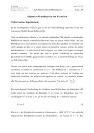
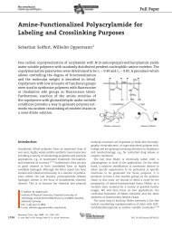
FIG. 1. Shift <strong>of</strong> <strong>frequency</strong> <strong>and</strong> b<strong>and</strong>width induced by a water droplet panels<br />
a <strong>and</strong> b <strong>and</strong> a hemispherical cap <strong>of</strong> a polymer gel panels c <strong>and</strong> d.<br />
The gel was produced by swelling the triblock copolymer Kraton G 1650 in<br />
light mineral oil at polymer-solvent ratio <strong>of</strong> 1:3. In the first case, the area<br />
was varied by just letting the droplet evaporate, while in the second, the area<br />
is a function <strong>of</strong> the vertical pressure applied to the stamp. The contact area<br />
was determined with a microscope imaging the sample from above adapted<br />
from Ref. 18.<br />
Application <strong>of</strong> Eq. 1 to the experimental data entails a<br />
complication because the contact area, A c , has to be measured<br />
in one way or another. This measurement usually requires<br />
a JKR tester, which, in turn, requires a transparent<br />
sample. Importantly, the contact area can be eliminated from<br />
the data analysis by considering the ratio <strong>of</strong> <strong>and</strong> −f,<br />
termed “D-f ratio.” Since <strong>and</strong> f should, according to<br />
the sheet-contact model, scale with contact area in the same<br />
way, the ratio should reflect a material’s parameter, regardless<br />
<strong>of</strong> the value <strong>of</strong> A c . A similar approach to data analysis<br />
was previously proposed in the context <strong>of</strong> QCM<br />
microweighing, 16 where the ratio <strong>of</strong> <strong>and</strong> −f is independent<br />
<strong>of</strong> film thickness for very thin films <strong>and</strong> closely related<br />
to the film’s elastic compliance, J. 17 The sheet-contact<br />
model predicts<br />
<br />
− f = cot 2,<br />
where =arctanG/G is the loss angle.<br />
Experiments with small droplets <strong>of</strong> water as well as<br />
hemispherical caps <strong>of</strong> polymer gels have shown that the D-f<br />
ratio does in some cases slightly depend on the contact<br />
radius. 18 Figure 1 displays two examples. The data in panels<br />
a <strong>and</strong> b were obtained by letting a water droplet evaporate<br />
3<br />
Downloaded 22 Sep 2010 to 139.174.150.114. Redistribution subject to AIP license or copyright; see http://jap.aip.org/about/rights_<strong>and</strong>_permissions
114909-3 Herrscher Ziegler, <strong>and</strong> Johannsmann J. Appl. Phys. 101, 114909 2007<br />
<strong>and</strong> measuring f, , <strong>and</strong> A c as a function <strong>of</strong> time. Panel<br />
a displays f <strong>and</strong> vs A c . Both f <strong>and</strong> are about<br />
proportional to area, but there are systematic deviations. By<br />
plotting the ratio /−f vs A c panel b, the deviations<br />
become more evident. Note that an incorrect determination<br />
<strong>of</strong> the contact area would not have shifted the ratio <strong>of</strong> <br />
<strong>and</strong> −f. Since it is hard to see how the loss angle <strong>of</strong> water<br />
close to 90° should depend on the droplet size, one concludes<br />
that some artifact comes into play. Panels c <strong>and</strong> d<br />
display analogous data obtained on a polymer gel Kraton G<br />
1650, swollen in light mineral oil, polymer weight fraction<br />
25%. In this case various degrees <strong>of</strong> vertical pressure were<br />
applied in order to adjust the contact area.<br />
The first shortcoming <strong>of</strong> the sheet-contact model coming<br />
to mind is acoustic scattering <strong>of</strong> the wave from the contact.<br />
Acoustic scattering is not captured by Eq. 1, because it<br />
assumes plane waves. This explanation was elaborated on in<br />
Ref. 18. A second effect—investigated here—is a change <strong>of</strong><br />
energy trapping induced by contacting the <strong>crystal</strong> in the center<br />
only. 19 Most <strong>crystal</strong>s are shaped such that the acoustic<br />
thickness is higher in the center than at the rim. The <strong>crystal</strong><br />
forms an acoustic lens which focuses the acoustic radiation<br />
to the center <strong>of</strong> the <strong>crystal</strong>. Acoustic focusing can be<br />
achieved by either employing convexly shaped <strong>crystal</strong>s<br />
which is common in the <strong>frequency</strong> control community or<br />
by employing thick, keyhole shaped electrodes. The latter<br />
configuration is more common in sensing. Usually, the back<br />
electrode is thicker <strong>and</strong> smaller than the front electrode, ensuring<br />
that the edge <strong>of</strong> the front electrode is outside the active<br />
area <strong>of</strong> sensing. Importantly, the strength <strong>of</strong> energy trapping<br />
is changed, when a load is applied in the center <strong>of</strong> the<br />
<strong>crystal</strong> only. When touching the <strong>crystal</strong> in the center, one<br />
applies a phase shift to the central acoustic beam, thereby<br />
changing the effective curvature <strong>of</strong> the acoustic lens. A<br />
change in energy trapping, in turn, changes the resonance<br />
<strong>frequency</strong>. As is shown below, the effect is substantial <strong>and</strong><br />
can account for area dependence <strong>of</strong> the D-f ratio. Strong<br />
energy trapping leads to strong shear gradients in the plane<br />
<strong>of</strong> the <strong>crystal</strong>, which increase the strain energy <strong>of</strong> the resonating<br />
structure. Even though the in-plane shear gradients are<br />
much weaker than the gradients along the surface normal,<br />
the effect, which energy trapping has on the resonance <strong>frequency</strong>,<br />
definitely is measurable. 20<br />
In order to discriminate between the effects <strong>of</strong> acoustic<br />
scattering, on the one h<strong>and</strong>, <strong>and</strong> <strong>of</strong> energy trapping, on the<br />
other, finite element method FEM simulations <strong>of</strong> partially<br />
loaded <strong>quartz</strong> <strong>crystal</strong>s were performed. Within a finite element<br />
simulation, the device <strong>of</strong> interest is divided into a discrete<br />
mesh. The equations <strong>of</strong> continuum mechanics are<br />
solved for these elements. FEM simulations on <strong>quartz</strong> <strong>resonators</strong><br />
are quite dem<strong>and</strong>ing because <strong>of</strong> the high Q factor. 21<br />
Most FEM simulations performed to date targeted the performance<br />
<strong>of</strong> <strong>resonators</strong> as acoustic clocks. 22,23 A prime concern<br />
is the separation <strong>of</strong> the main resonance from the anharmonic<br />
sideb<strong>and</strong>s the “spurious modes”, which can be achieved by<br />
optimization <strong>of</strong> the geometry. Other topics <strong>of</strong> interest were<br />
the effects <strong>of</strong> gravity <strong>and</strong> stress. An FEM simulation in the<br />
context <strong>of</strong> sensing was reported by Friedt et al. 24 These authors<br />
looked into the flexural contribution to the displacement<br />
pattern by means <strong>of</strong> static simulations.<br />
FEM simulations allow us to distinguish between effects<br />
<strong>of</strong> energy trapping, on the one h<strong>and</strong>, <strong>and</strong> scattering, on the<br />
other, because they provide the amplitude distribution <strong>and</strong><br />
the distribution <strong>of</strong> shear gradients. These are difficult to determine<br />
in experiment. Also, one can easily simulate samples<br />
with very small contact areas. In experiment, the <strong>frequency</strong><br />
shift induced by very small contacts radius <strong>of</strong> contact<br />
100 m cannot be measured with sufficient accuracy. As<br />
we show below, both acoustic scattering <strong>and</strong> a change <strong>of</strong><br />
energy trapping do play a role, but they do so in different<br />
ranges <strong>of</strong> contact size.<br />
The influence <strong>of</strong> energy trapping can also be calculated<br />
analytically based on perturbation theory. The small perturbation<br />
parameter is the contact area, A c , divided by the active<br />
area <strong>of</strong> the <strong>crystal</strong>, A. The first order perturbation result<br />
yields a term proportional to A c <strong>and</strong> is equivalent to the<br />
sheet-contact model. The second order result contains a term<br />
proportional to A c 2 <strong>and</strong> produces a deviation from the sheetcontact<br />
model. For an idealized geometry, the theory makes a<br />
quantitative prediction for size <strong>of</strong> the deviation. For realistic<br />
geometries, the result needs to be augmented with a numerical<br />
factor <strong>of</strong> order unity.<br />
FEM simulations<br />
For the sake <strong>of</strong> computational efficiency, the simulations<br />
were limited to a two-dimensional representation <strong>of</strong> the <strong>crystal</strong>,<br />
rather than a three-dimensional object. Leaving away the<br />
third dimension, we certainly sacrifice the claim to a truly<br />
realistic simulation. The simulation still elucidates the role <strong>of</strong><br />
acoustic scattering <strong>and</strong> <strong>of</strong> energy trapping. In order to ensure<br />
that the simulation matches the experiment, a few checks<br />
were performed in selected cases. For instance, both the<br />
Sauerbrey equation 3 <strong>and</strong> the Borovikov-Kanazawa-Gordon<br />
result 7,8 were confirmed when bringing the resonator into<br />
contact with a thin film <strong>and</strong> a semi-infinite liquid, respectively.<br />
Detailed investigations to confirm the validity <strong>of</strong> the<br />
two-dimensional simulations are part <strong>of</strong> future research.<br />
The simulations were carried out with the s<strong>of</strong>tware package<br />
FEMLAB 3.0 COMSOL AB, Stockholm, Sweden, which<br />
included the Structural Mechanics Extension module. In a<br />
first step, a static piezoelectric simulation was performed using<br />
the Multiphysics module. From this simulation, the relation<br />
between the external voltage <strong>and</strong> the stress distribution<br />
inside the resonator was obtained. In the following steps, this<br />
stress distribution multiplied by cost was used as the<br />
excitation field, rather than the electric voltage. In this way,<br />
the use <strong>of</strong> the piezoelectric tensor in the main simulation was<br />
avoided. The latter was based on conventional elasticity.<br />
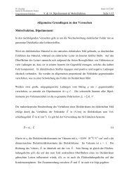
The simulations were performed on a cross section <strong>of</strong> a<br />
<strong>quartz</strong> <strong>crystal</strong> oscillator as schematically shown in Fig. 2.<br />
The slab corresponds to a cut through an AT-cut, planar<br />
<strong>quartz</strong> disk along the x axis. The radius <strong>of</strong> the plate is 10 mm<br />
<strong>and</strong> its thickness is 166 m, resulting in a fundamental resonance<br />
<strong>frequency</strong> <strong>of</strong> 10 MHz. The <strong>crystal</strong> is clamped at the<br />
edge by imposing that the displacement be zero outside r<br />
Downloaded 22 Sep 2010 to 139.174.150.114. Redistribution subject to AIP license or copyright; see http://jap.aip.org/about/rights_<strong>and</strong>_permissions
114909-4 Herrscher Ziegler, <strong>and</strong> Johannsmann J. Appl. Phys. 101, 114909 2007<br />
FIG. 2. Discretization mesh used in the FEM simulation. The drawing is not<br />
to scale.<br />
=9.5 mm. The electrodes had a thickness <strong>of</strong> 100 nm <strong>and</strong> a<br />
radius <strong>of</strong> 7 mm. The material parameters were chosen to<br />
mimic gold. In order to analyze the influence <strong>of</strong> a partial<br />
loading <strong>of</strong> the <strong>quartz</strong>, a cylinder <strong>of</strong> the respective material<br />
was placed onto the center <strong>of</strong> the top electrode. The parameters<br />
<strong>of</strong> the applied materials are listed in Table I. The height<br />
<strong>of</strong> the sample was 10 m. The height must be larger than the<br />
penetration depth <strong>of</strong> the shear wave in order to ensure that<br />
the shear oscillation does not reach the outer interface. Reflections<br />
<strong>of</strong> acoustic waves from the back <strong>of</strong> the <strong>crystal</strong> can<br />
then be ignored.<br />
The mesh divides the <strong>crystal</strong> into finite elements, inside<br />
which displacement <strong>and</strong> stress are interpolated with shape<br />
functions. It is essential to adapt the mesh size distribution to<br />
the problem under investigation. Figure 2 shows the mesh<br />
employed in this work. The elements are small at the top, at<br />
the bottom, <strong>and</strong> in the center <strong>of</strong> the <strong>crystal</strong>. Even though the<br />
outcome <strong>of</strong> the simulation should not critically be affected<br />
by the anisotropy <strong>of</strong> the <strong>crystal</strong>, anisotropic elastic parameters<br />
were employed. Piezoelectrically stiffened shear<br />
moduli were applied. 25 The values inserted into the model<br />
were c¯11 =86.74 GPa, c¯12 =−8.27 GPa, c¯22 =129.8 GPa, <strong>and</strong><br />
c¯66 =29.24 GPa. The bars indicate that these parameters were<br />
obtained after rotating the coordinate system about the y axis<br />
by 35° in order to describe the AT cut.<br />
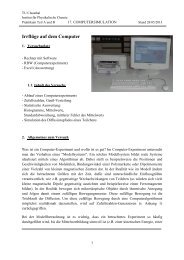
Frequency <strong>and</strong> b<strong>and</strong>width <strong>of</strong> the <strong>crystal</strong> were derived by<br />
means <strong>of</strong> a simulated <strong>frequency</strong> sweep. Figure 3 shows the<br />
area-averaged amplitude at the top <strong>of</strong> the <strong>crystal</strong>, uf, asa<br />
function <strong>of</strong> driving <strong>frequency</strong>. Panels a <strong>and</strong> b show a<br />
slightly damped Q=160 000 <strong>and</strong> a heavily damped Q<br />
=730 <strong>crystal</strong>, respectively. In the latter case, the main resonance<br />
overlaps with an anharmonic sideb<strong>and</strong>. The function<br />
uf was fitted with a resonance curve <strong>of</strong> the form<br />
TABLE I. Material parameters.<br />
g/cm 3 mPa s mPa s<br />
Water 1 1.0 0<br />
Elastomer 1 1.0 1.59<br />
Solid Film 1 0 159 000 G=10 GPa<br />
FIG. 3. Simulated resonance curves for a weakly loaded <strong>crystal</strong> Q<br />
=160 000, panel a <strong>and</strong> a heavily loaded <strong>crystal</strong> Q=730, panel b. Inthe<br />
latter case, the main resonance overlaps with an anharmonic sideb<strong>and</strong>. The<br />
dotted line is the fit with a single resonance curve. In panel a, the simulation<br />
<strong>and</strong> the fit with a resonance curve cannot be distinguished.<br />
uf =<br />
C<br />
f0 2 − f 2 2 + 2f 2 ,<br />
where C is a prefactor, f 0 is the resonance <strong>frequency</strong>, f is the<br />
excitation <strong>frequency</strong>, <strong>and</strong> describes the width <strong>of</strong> the curve.<br />
The parameter is equal to half the b<strong>and</strong>width at half maximum<br />
<strong>of</strong> the imaginary part <strong>of</strong> uf where the latter is proportional<br />
to the conductance <strong>of</strong> the <strong>crystal</strong>, G, <strong>and</strong> therefore<br />
is the basis <strong>of</strong> impedance analysis. The FEM analysis<br />
makes use <strong>of</strong> the modulus uf, in which case is the half<br />
b<strong>and</strong>width at 1/2 1/2 <strong>of</strong> the peak height. The simulated sweep<br />
is performed for both the unloaded <strong>and</strong> the loaded <strong>crystal</strong> in<br />
order to find the shifts, f <strong>and</strong> . The parameters f norm<br />
<strong>and</strong> norm are defined as<br />
r Q<br />
u 2 xdx<br />
f norm = f L − f u A Q<br />
= f L − f u −r<br />
r<br />
A<br />
C<br />
,<br />
c<br />
u 2 xdx<br />
−r C<br />
r Q<br />
u 2 xdx<br />
norm = L − u A Q<br />
= L − u −r<br />
r<br />
A<br />
C<br />
,<br />
c<br />
u 2 xdx<br />
−r C<br />
where the indices L <strong>and</strong> u denote the loaded <strong>and</strong> unloaded<br />
<strong>crystal</strong>s, respectively, r Q is the radius <strong>of</strong> the <strong>crystal</strong>, r C<br />
is the<br />
radius <strong>of</strong> contact, <strong>and</strong> ux is the amplitude <strong>of</strong> oscillation at<br />
position x. The terms in the numerator <strong>and</strong> the denominator<br />
are the active area, A, <strong>and</strong> contact area, A c , respectively. If<br />
the sheet-contact model were rigorously correct, the normalized<br />
shifts <strong>of</strong> <strong>frequency</strong> <strong>and</strong> b<strong>and</strong>width as a function <strong>of</strong> contact<br />
radius would approach a horizontal line for A C<br />
A. The<br />
values <strong>of</strong> f norm <strong>and</strong> norm would obey the Sauerbrey <strong>and</strong><br />
the Borovikov-Kanazawa equation for a film <strong>and</strong> a liquid,<br />
respectively.<br />
4<br />
5<br />
Downloaded 22 Sep 2010 to 139.174.150.114. Redistribution subject to AIP license or copyright; see http://jap.aip.org/about/rights_<strong>and</strong>_permissions
114909-5 Herrscher Ziegler, <strong>and</strong> Johannsmann J. Appl. Phys. 101, 114909 2007<br />
Energy trapping for convexly shaped <strong>crystal</strong>s<br />
The change <strong>of</strong> energy trapping <strong>and</strong> the consequences <strong>of</strong><br />
such changes can be calculated by means <strong>of</strong> a perturbation<br />
approach, which borrows from the quantum mechanical<br />
treatment <strong>of</strong> the harmonic oscillator. The mathematics described<br />
below applies to plane convexly shaped <strong>crystal</strong>s. As<br />
in the FEM simulation, we treat the two-dimensional slab.<br />
The result can be transferred to other geometries by changing<br />
a numerical factor.<br />
Let the shape <strong>of</strong> the lower <strong>crystal</strong> surface be parabolic.<br />
Plane-convex <strong>crystal</strong>s are, in fact, employed extensively in<br />
the <strong>frequency</strong> control community. These <strong>crystal</strong>s have better<br />
energy trapping on the fundamental than the planar <strong>crystal</strong>s<br />
usually employed in sensing. 26,27 Let d q be the thickness in<br />
the center <strong>of</strong> the <strong>crystal</strong> <strong>and</strong> let the radius <strong>of</strong> curvature, R, be<br />
much larger than the thickness. The <strong>crystal</strong> is assumed to be<br />
“locally flat,” meaning that all gradients in the surface plane<br />
are much smaller than the gradients along the vertical. The<br />
displacement pattern is given by a st<strong>and</strong>ing wave, where the<br />
vertical component <strong>of</strong> the wave number, k z x, at each location,<br />
x, is equal to n/dx, where n is the overtone order.<br />
The displacement pattern, Ux,z, is approximated as<br />
Ux,z = u 0 sin n<br />
dx z ux,<br />
where u 0 is an amplitude with dimension <strong>of</strong> a length. The<br />
function ux describing the amplitude distribution along x is<br />
dimensionless. The wave equation is<br />
2 U + 2<br />
c 2 U = − k 2 z x + 2<br />
x 2 + 2<br />
c 2u 0 uxsin <br />
n<br />
dx z<br />
6<br />
=0, 7<br />
where c is the speed <strong>of</strong> sound. The wave vector along the<br />
surface normal, k z , depends on location, x. For a planeconvex<br />
<strong>crystal</strong>, dx is given by d q 1−x 2 /2Rd q , resulting<br />
in<br />
k z x<br />
n<br />
d q 1−x 2 /2Rd q n<br />
d q1+<br />
x2<br />
2Rd q.<br />
Further, for x 2 Rd q , the square <strong>of</strong> k z can be simplified to<br />
k 2 z x n<br />
d q<br />
21+ x2<br />
9<br />
Rd q,<br />
which yields<br />
− 2 u<br />
<br />
x 2 + n<br />
d q<br />
21+ x2<br />
Rd q − 2<br />
c 2u<br />
=− 2 u<br />
x 2 +x2<br />
<br />
4<br />
− u =0.<br />
10<br />
The eigenvalue, , is defined as<br />
8<br />
= 2<br />
c 2<br />
n<br />
−<br />
2<br />
d q<br />
. 11<br />
has the dimension <strong>of</strong> an inverse square length. The parameter<br />
is given by<br />
4 = Rd 3<br />
q<br />
n 2 .<br />
12<br />
Equation 10 is known from the quantum theory <strong>of</strong> the harmonic<br />
oscillator. 28 It resembles the Schrödinger equation,<br />
where 2 u/x 2 would be proportional to the kinetic energy<br />
<strong>and</strong> x 2 / 4 would be the potential. Its solutions are<br />
u 0 m x = a 0 m H m<br />
exp x − x2<br />
2 2.<br />
13<br />
The superscript 0 denotes the zeroth perturbation order.<br />
H m x are the Hermite polynomials <strong>and</strong> a 0 m<br />
are normalization<br />
constants. In the context <strong>of</strong> <strong>quartz</strong> <strong>crystal</strong> <strong>resonators</strong>, the<br />
index m labels the anharmonic sideb<strong>and</strong>s as opposed to the<br />
overtone orders, which are labeled by n. The lowest Hermite<br />
polynomial is H 0 =1; the corresponding solution is the<br />
Gaussian. Higher Hermite polynomials contain nodes in the<br />
lateral amplitude distribution. These solutions correspond to<br />
the anharmonic sideb<strong>and</strong>s. Here, only the main resonances<br />
are <strong>of</strong> interest, which have m=0.<br />
The solutions are normalized such that<br />
<br />
−<br />
<br />
u 0 m x 2 dx =−<br />
1.<br />
a m 0 2H m x 2<br />
exp− x2<br />
2dx<br />
14<br />
The parameter a m 0 2 has the dimension <strong>of</strong> an inverse<br />
length, termed “active area,” A. The active area here has<br />
dimension <strong>of</strong> a length, since a two-dimensional slab is considered,<br />
rather than a three-dimensional plate. The active<br />
area can be written as<br />
<br />
A = a 0 0 −2 =−<br />
exp− x2<br />
2dx = .<br />
15<br />
For modes with m0, the normalizing factors contain a numerical<br />
coefficient, m , given as<br />
a 0 m = m 1 1<br />
= .<br />
A 2 m m! A<br />
The eigenvalues 0 m<br />
are given by<br />
m 0 = 2m +1 1 2 .<br />
16<br />
17<br />
The resonance <strong>frequency</strong> <strong>of</strong> the hypothetical flat resonator<br />
R= is defined as ¯ =2f 0 =cn/d q . In the following, the<br />
resonance <strong>frequency</strong> is written as =¯ +˜ , where ˜ is a<br />
<strong>frequency</strong> shift. ˜ can be calculated by perturbation theory.<br />
The zeroth order term, ˜ 0 , only comprises the correction<br />
due to energy trapping. The first order contribution, ˜ 1 , will<br />
be the <strong>frequency</strong> shift induced by the sample as predicted by<br />
the sheet-contact model. The second order contribution, ˜ 2 ,<br />
will be caused by the change <strong>of</strong> energy trapping due to the<br />
presence <strong>of</strong> the sample. The second order term will turn out<br />
Downloaded 22 Sep 2010 to 139.174.150.114. Redistribution subject to AIP license or copyright; see http://jap.aip.org/about/rights_<strong>and</strong>_permissions
114909-6 Herrscher Ziegler, <strong>and</strong> Johannsmann J. Appl. Phys. 101, 114909 2007<br />
to be the source <strong>of</strong> the area dependence <strong>of</strong> the D-f ratio.<br />
We first treat the zeroth order approximation. Assuming<br />
˜ 0 m<br />
¯ , 2 m can be approximated as<br />
2 m ¯ + ˜ 0 m 2 ¯ 2 +2¯ ˜ 0 m .<br />
18<br />
Using these variables <strong>and</strong> Eq. 11, Eq. 17 reads<br />
0 m = 2<br />
m<br />
c 2 − ¯ 2<br />
c 2 = 2<br />
2<br />
m n<br />
−<br />
c 2 d q = 2¯ ˜ 0<br />
m<br />
c 2 = 2m +1 1 2 .<br />
19<br />
The eigenvalues have dimension <strong>of</strong> an inverse square length,<br />
whereas the fundamental quantity in QCM measurements is<br />
a <strong>frequency</strong>. One translates between the two by multiplying<br />
with c 2 /2¯ ,<br />
˜ 0 m = 1<br />
2¯ 2 m − ¯ 2 = 2m +1<br />
2¯ 2 = 2m +1 tr. 20<br />
The quantity tr denotes the <strong>frequency</strong> increase caused by<br />
energy trapping the “vibrational <strong>frequency</strong>” in the context <strong>of</strong><br />
quantum mechanics, not be confused with the resonance <strong>frequency</strong><br />
<strong>of</strong> the <strong>crystal</strong>. The contribution <strong>of</strong> the transverse<br />
shear gradients to the <strong>frequency</strong> is sizable, as can be seen<br />
from the ratio <strong>of</strong> tr /¯ for m=0,<br />
tr<br />
¯ = c 2<br />
2<br />
2¯ 2 2 = d q<br />
2n 2 2 .<br />
21<br />
Using d q =166 m, =1.66 mm, <strong>and</strong> n=1 yields tr /2<br />
=1/2 2 0.0110 MHz5 kHz. A change <strong>of</strong> energy trapping<br />
can easily produce a <strong>frequency</strong> shift <strong>of</strong> a few hertz. As a side<br />
result, we mention that the change <strong>of</strong> energy trapping is unessential<br />
in the simple Sauerbrey case. This can be seen by<br />
comparing the shift in tr to the shift in ¯ when the thickness<br />
<strong>of</strong> the <strong>crystal</strong> is increased by a small amount, d q . The detailed<br />
calculation shows that<br />
tr<br />
¯ = 1 tr<br />
2 ¯ .<br />
22<br />
The contribution <strong>of</strong> energy trapping to the Sauerbrey result is<br />
<strong>of</strong> the order <strong>of</strong> 10 −3 <strong>and</strong> may be neglected in view <strong>of</strong> the<br />
other uncertainties in microweighing.<br />
Touching the <strong>crystal</strong> in the center amounts to small perturbation.<br />
It is assumed that the contact area is larger than the<br />
thickness <strong>of</strong> the <strong>crystal</strong>, so that the vertical <strong>and</strong> the horizontal<br />
scale still separate well. The effect <strong>of</strong> the sample is introduced<br />
into Eq. 7 by modifying the parameter k z x. Dissipation<br />
is introduced by making k z x complex in the region<br />
<strong>of</strong> contact. The shift <strong>of</strong> the k vector induced by the load is<br />
inferred from the flat-plate analog: According to the small<br />
load approximation, 29 the complex fractional <strong>frequency</strong> shift<br />
is<br />
f + i<br />
= i Z L .<br />
23<br />
f f Z q<br />
The parameter Z L here is the load impedance, which is<br />
the ratio <strong>of</strong> stress <strong>and</strong> speed at the <strong>crystal</strong> surface. f f is the<br />
<strong>frequency</strong> <strong>of</strong> the fundamental. Using the <strong>frequency</strong> <strong>of</strong> the<br />
c 2<br />
unperturbed <strong>crystal</strong> at the given overtone order, f 0 =nf f , instead<br />
<strong>of</strong> the <strong>frequency</strong> <strong>of</strong> the fundamental, the small load<br />
approximation reads<br />
f + i i<br />
= Z L .<br />
24<br />
f 0 nZ q<br />
When the sample is a flat punch <strong>of</strong> a viscoelastic material,<br />
the load impedance is the same as the acoustic impedance <strong>of</strong><br />
the sample, Z ac =G 1/2 . The perturbation calculation would<br />
also apply if the load were <strong>of</strong> some other nature such as a<br />
Sauerbrey film.<br />
A complex <strong>frequency</strong> shift as given by Eq. 23 implies<br />
a complex wave vector for the loaded <strong>crystal</strong> given by<br />
k z,L x = k z x + k z x = k z x + k z x iZ Lx<br />
, 25<br />
nZ q<br />
where the index L denotes the loaded <strong>crystal</strong> <strong>and</strong> k z is the<br />
2<br />
shift <strong>of</strong> k z induced by the load. For k z,L we find<br />
k 2 z,L x = k z x + k z x 2 k 2 z x +2k z xk z x<br />
= k 2 z x + k 2 z x 2iZ Lx<br />
. 26<br />
nZ q<br />
This yields the wave equation<br />
− 2 u<br />
x 2 + n2 2<br />
2 1+ x2 2iZ Lx<br />
d q<br />
Rd q1+<br />
nZ q<br />
<br />
=− 2 u<br />
x 2 + x2<br />
+ n2 2<br />
d q<br />
2<br />
41+ 2iZ Lx<br />
nZ q<br />
<br />
− 2<br />
c 2u<br />
− 2<br />
c 2u<br />
+ n2 2 2iZ L x<br />
2<br />
d q<br />
nZ q<br />
− 2 u<br />
<br />
x 2 + x2<br />
4 + n2 2 2Z L x<br />
2<br />
− u =0. 27<br />
d q<br />
nZ q<br />
Equation 12 has been used when replacing n 2 2 /Rd 3 q by<br />
−4 . The relation Z L Z q was used in line 3 square brackets<br />
in line 2 replaced by unity. Below, it will be convenient to<br />
use eigenvalues with a dimension <strong>of</strong> a <strong>frequency</strong> termed ˜ .<br />
This is achieved by multiplying Eq. 27 with c 2 /2¯ cf.<br />
Eq. 20;<br />
− c2<br />
2¯<br />
2<br />
c2<br />
x2u +<br />
2¯<br />
1<br />
4x2 u + ¯ iZ Lx<br />
nZ q<br />
u − ˜ u =0.<br />
28<br />
In Eq. 28 ¯ =cn/d q was used. With regard to the algebraic<br />
details <strong>of</strong> the perturbation analysis, the approach from<br />
Ref. 30 is applied. Before proceeding, we cast Eq. 28 into<br />
a form matching the choices made there. Reference 30 uses<br />
the bracket notation<br />
H 0 + Vm = E m m,<br />
29<br />
where is the small perturbation parameter, H 0 is the Hamiltonian<br />
operator, V is a perturbing potential, m is a state, <strong>and</strong><br />
E m is an eigenvalue. In quantum mechanics, the eigenvalues<br />
have the dimension <strong>of</strong> an energy, whereas they are frequencies<br />
here. Comparing Eqs. 29 <strong>and</strong> 28 the following correspondences<br />
are found:<br />
Downloaded 22 Sep 2010 to 139.174.150.114. Redistribution subject to AIP license or copyright; see http://jap.aip.org/about/rights_<strong>and</strong>_permissions
114909-7 Herrscher Ziegler, <strong>and</strong> Johannsmann J. Appl. Phys. 101, 114909 2007<br />
H 0 =− c2<br />
2¯<br />
2<br />
x 2 + c2<br />
2¯<br />
1<br />
4 ,<br />
V = i¯ Z Lx<br />
nZ q<br />
,<br />
m = u m x,<br />
30<br />
E m = ˜ m.<br />
Importantly, V is not a Hermitian operator, <strong>and</strong> as a consequence<br />
kVmmVk * . 31 Because V is not Hermitian, the<br />
eigenvalues, ˜ m, are complex: they contain a <strong>frequency</strong> shift<br />
as well as an increase in b<strong>and</strong>width that is, an imaginary<br />
part. Borrowing from Ref. 30 we write<br />
m = m 0 + m 1 + ¯ ,<br />
31<br />
m = E m − E 0 m = ˜ m − ˜ 0 m = 1 m + 2 2 m + ¯ ,<br />
m 1 = m 0 Vm 0 ,<br />
32<br />
33<br />
m 1 = k 0 k0 Vm 0 <br />
km E 0 0<br />
, 34<br />
m − E k<br />
<strong>and</strong><br />
2 m = m 0 Vm 1 m<br />
= <br />
0 Vk 0 k 0 Vm 0 <br />
km E 0 0<br />
. 35<br />
m − E k<br />
Only the terms with m 0 =0 are <strong>of</strong> interest, because the main<br />
resonance is used for measurement. The anharmonic sideb<strong>and</strong>s<br />
are essential in the calculation because the eigenstate<br />
in the presence <strong>of</strong> the sample m 1 contains contributions<br />
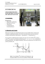
from k0 Eq. 34. This fact is illustrated in Fig. 4b.<br />
When superimposing the states 0 <strong>and</strong> 3 with relative<br />
weights <strong>of</strong> 0.9 <strong>and</strong> 0.1, respectively, an amplitude distribution<br />
is obtained, which looks different from the state 0 in<br />
the sense that it has a somewhat sharper peak in the center.<br />
This is what is found in the simulation, as well Fig. 4a.<br />
Setting m 0 =0 <strong>and</strong> inserting Eq. 30 into Eq. 33<br />
yields the first order result for the <strong>frequency</strong> shift,<br />
1 0 =0 i¯ Z <br />
Lx<br />
0<br />
u i¯ Z Lx<br />
nZ 0 u 0<br />
q<br />
nZ 0 dx<br />
q<br />
=<br />
i¯<br />
<br />
AnZ q<br />
−<br />
0 =−<br />
Z L xexp− x2<br />
2dx.<br />
36<br />
For a contact with a viscoelastic medium, Z L x is constant<br />
<strong>and</strong> equal to Z L =Z ac =G 1/2 between −r c <strong>and</strong> r c r c the<br />
contact radius. If the contact radius is much smaller than the<br />
radius <strong>of</strong> the active area, exp−x 2 / 2 can be approximated<br />
by unity. In the language <strong>of</strong> the sheet-contact model, this<br />
implies K A r c 1. This leads to<br />
f* 1 = f 1 + i 1 = 0 1<br />
2 = f 2r c iZ L<br />
0 . 37<br />
A nZ q<br />
Here, f 0 ¯ /2/2 is the <strong>frequency</strong> <strong>of</strong> the unperturbed<br />
resonator. Identifying 2r c with the contact area, A c ,<br />
FIG. 4. a Amplitude distribution <strong>of</strong> a bare <strong>crystal</strong> full line <strong>and</strong> a <strong>crystal</strong><br />
loaded with a water droplet r c =1 mm, dotted line. The load modifies the<br />
amplitude distribution <strong>and</strong> introduces additional lateral shear gradients.<br />
Panel b illustrates how a cusp in the center <strong>of</strong> the amplitude distribution<br />
can be produced by mixing the main resonance with a contribution from the<br />
third anharmonic sideb<strong>and</strong>.<br />
<strong>and</strong>, also, substituting nf f for f 0 , Eq. 37 becomes equivalent<br />
to the sheet-contact model Eq. 2.<br />
Having rederived the sheet-contact model in this somewhat<br />
complicated way, we feel encouraged to move forward<br />
to the second order term. The first order displacement pattern<br />
is given by<br />
0 1 = k 0 k0 V0 0 <br />
k0 E 0 0<br />
0 − E .<br />
k<br />
The functions k 0 are<br />
k 0 = k<br />
A<br />
H k x exp − x2<br />
2 2.<br />
The term in the denominator is Eq. 20<br />
1<br />
E 0 0<br />
0 − E =− 1 .<br />
k<br />
2k tr<br />
The scalar product k 0 V0 0 is<br />
k 0 V0 0 = i¯ Z L<br />
nZ q<br />
1<br />
A−r c<br />
exp− x2<br />
2dx.<br />
r c<br />
k H k x H 0 x <br />
In order to solve the integral, we substitute x by =x/,<br />
38<br />
39<br />
40<br />
41<br />
Downloaded 22 Sep 2010 to 139.174.150.114. Redistribution subject to AIP license or copyright; see http://jap.aip.org/about/rights_<strong>and</strong>_permissions
114909-8 Herrscher Ziegler, <strong>and</strong> Johannsmann J. Appl. Phys. 101, 114909 2007<br />
FIG. 5. Shift <strong>of</strong> <strong>frequency</strong> f norm <strong>and</strong> <strong>of</strong> b<strong>and</strong>width norm <strong>of</strong> a <strong>crystal</strong><br />
loaded with a droplet <strong>of</strong> water. The lines are fits to Eq. 50 with B <strong>and</strong> B <br />
as a free parameters.<br />
r c /<br />
k 0 V0 0 = i¯ Z L<br />
nZ q A k H k H 0 exp− −r 2 d.<br />
c /<br />
42<br />
The second order correction 0 2 is given by<br />
2 0 = 0 0 V0 1 0<br />
= <br />
0 Vk 0 k 0 V0 0 <br />
k0 E 0 0<br />
0 − E k<br />
=− ¯ Z L<br />
nZ q2<br />
<br />
k0<br />
r c /<br />
−r c /<br />
1<br />
− tr <br />
2<br />
A 2 1<br />
2k<br />
k H k H 0 exp− 2 d2. 43<br />
The integral can be evaluated with s<strong>of</strong>tware packages such as<br />
MATHEMATICA. The outcome is<br />
r c /<br />
−r c /<br />
k H k H 0 exp− 2 d<br />
<br />
= 2k Fk/2,3/2,− rc / 2 <br />
, 44<br />
2 k k!1−k/2<br />
where F is the generalized hypergeometric function <strong>and</strong> the<br />
Gamma-function x not to be confused with the b<strong>and</strong>width<br />
interpolates the factorial. Since only small contact<br />
areas are <strong>of</strong> interest, we exp<strong>and</strong> the square <strong>of</strong> the integral to<br />
second order in r c /,<br />
r c /<br />
−r c /<br />
<br />
k H k H 0 exp− 2 d2<br />
2<br />
2 k r 2<br />
c<br />
. 45<br />
k!1−k/2 <br />
Finally, the sum evaluates to<br />
FIG. 6. Shift <strong>of</strong> <strong>frequency</strong> f norm <strong>of</strong> half b<strong>and</strong>width at half maximum<br />
norm <strong>of</strong> a <strong>crystal</strong> loaded with a viscoelastic material. The lines are fits to<br />
Eq. 50 with B <strong>and</strong> B as a free parameters.<br />
<br />
<br />
k0<br />
1<br />
r c /<br />
2k−r c /<br />
k H k H 0 exp− 2 d2<br />
1.07 r 2<br />
c<br />
2 . 46<br />
Since the numerical factor <strong>of</strong> 1.07 depends on the geometry,<br />
we replace it with the variable B. Collecting the parameters<br />
yields<br />
2 0 = B ¯ Z L<br />
nZ q<br />
2 2<br />
1 r c<br />
tr A 2 .<br />
47<br />
Substituting r c =A c /2, ¯ =2nf f , 0 2 =2f* 2 ,<br />
tr =c 2 /2¯ 2 , <strong>and</strong> c=2d q f f leads to<br />
f* 2<br />
f f<br />
= B Z L<br />
2 2<br />
A c<br />
Z q<br />
2<br />
A 2 2 n<br />
2d q<br />
2 .<br />
48<br />
Collecting the results from the first <strong>and</strong> the second order<br />
yields<br />
f*<br />
f f<br />
= f*1 + f* 2<br />
f f<br />
= A c<br />
A<br />
iZ L<br />
+ B Z L<br />
Z q<br />
2 2<br />
A c<br />
Z q<br />
2<br />
A 2 2 n<br />
2d q<br />
2<br />
= A c iZ Z L<br />
L A c 2 n<br />
A Z q1−iB<br />
Z q A 2d<br />
2.<br />
49<br />
q<br />
The equations simplify, if 2 is expressed in terms <strong>of</strong> the<br />
active area. We need to treat the two-dimensional slab <strong>and</strong><br />
the three-dimensional plate separately. For the twodimensional<br />
slab, is replaced by A using Eq. 15. Further,<br />
we separate the real <strong>and</strong> the imaginary part, which yields<br />
f<br />
f f<br />
<br />
f f<br />
=− A c<br />
A<br />
= A c<br />
A<br />
Z L 1 A c An<br />
2<br />
Z q1+B<br />
Z q 2d q<br />
Z L 1 A c An<br />
2<br />
Z q1+B<br />
Z q d q<br />
Z L 2 − Z L 2<br />
Z L .<br />
Z L <br />
,<br />
50<br />
Equation 50 is to be compared with the simulation data<br />
see Figs. 5–7 <strong>and</strong> Table II. The data are fitted with a function<br />
<strong>of</strong> the form<br />
Downloaded 22 Sep 2010 to 139.174.150.114. Redistribution subject to AIP license or copyright; see http://jap.aip.org/about/rights_<strong>and</strong>_permissions
114909-9 Herrscher Ziegler, <strong>and</strong> Johannsmann J. Appl. Phys. 101, 114909 2007<br />
FIG. 7. Shift <strong>of</strong> <strong>frequency</strong> f <strong>of</strong> half b<strong>and</strong>width at half maximum <strong>of</strong><br />
a <strong>crystal</strong> loaded with a Sauerbrey film. The line is a fit to Eq. 50 with B <br />
as a free parameter.<br />
f<br />
f f<br />
= 1+A c ,<br />
<br />
f f<br />
= 1+A c .<br />
51<br />
For the sake <strong>of</strong> comparison, the parameter B was allowed to<br />
be different for f <strong>and</strong> , that is, two parameters B <strong>and</strong> B<br />
are derived from experiment <strong>and</strong> simulation. B <strong>and</strong> B are<br />
computed from the fit parameters <strong>and</strong> . If the above<br />
analysis were strictly correct, B <strong>and</strong> B would take the same<br />
value.<br />
For the three-dimensional plate, the area, A, <strong>and</strong> 2 are<br />
related as<br />
A =−<br />
<br />
<br />
<br />
−<br />
exp− x2 + y 2<br />
2 dxdy = 2 . 52<br />
FIG. 8. Data from Fig. 1, displayed in analogy to Figs. 5–7. The lines are<br />
fitstoEq.53.<br />
f<br />
f f<br />
<br />
f f<br />
=− A c<br />
A<br />
= A c<br />
A<br />
Z L 1 A c n<br />
2<br />
Z q1+B<br />
Z q 2d q<br />
Z L 1 A c n<br />
2<br />
Z q1+B<br />
Z q d Z L .<br />
q<br />
Z L 2 − Z L 2<br />
Z L <br />
,<br />
53<br />
Using this result in Eq. 49 <strong>and</strong> again separating real <strong>and</strong><br />
imaginary parts lead to<br />
TABLE II. Normalized slopes <strong>and</strong> derived values for B.<br />
mm −1 B mm −1 B<br />
Simulation<br />
Water 0.011 0.099 0.51<br />
Elastomer −0.216 0.37 0.040 0.47<br />
Film 100 nm 0.055 0.50<br />
Expt.<br />
Water mm −2 B mm −2 B<br />
n=5 0.11 19.5 0.15 4.11<br />
n=7 0.10 7.72 0.15 2.19<br />
n=9 0.089 4.03 0.17 1.60<br />
n=11 0.050 1.64 0.13 0.84<br />
n=13 0.055 1.39 0.15 0.81<br />
Expt.<br />
Polymer gel<br />
n=3 0.10 −1.7 0.16 1.4<br />
n=5 −0.10 0.9 0.26 0.8<br />
n=7 −0.17 0.66 0.33 0.6<br />
Equation 53 is to be compared with experiment Fig. 8 <strong>and</strong><br />
Table II in the same way as Eq. 50 is compared to the<br />
simulation.<br />
Before moving on to the comparison with simulation <strong>and</strong><br />
experiment, we check that Eq. 53 produces an increase <strong>of</strong><br />
the D-f ratio with increasing contact area for the case <strong>of</strong> a<br />
water droplet Fig. 1b. For water, the <strong>frequency</strong> shift is unaffected<br />
by energy trapping because water has Z L<br />
=i 1/2 <strong>and</strong> therefore Z L =Z L . The b<strong>and</strong>width does increase,<br />
<strong>and</strong> so does the D-f ratio, /−f.<br />
Such a result should be also obtained with anisotropic<br />
three-dimensional plates <strong>and</strong> keyhole shaped back electrodes.<br />
Importantly, this change <strong>of</strong> dimension <strong>and</strong> geometry<br />
only affects the numerical factor B. The functions u m x in<br />
Eq. 13 turn into more complicated functions <strong>of</strong> radius, r,<br />
<strong>and</strong> angle, . Also, the frequencies <strong>of</strong> the anharmonic sideb<strong>and</strong>s<br />
will not be described by Eq. 20. This changes the<br />
elements <strong>of</strong> the sum in Eq. 43. The integral in Eq. 43 runs<br />
over an area, rather than a line, <strong>and</strong> its outcome must therefore<br />
be an area. Everything falls in place, if A <strong>and</strong> A c are<br />
reinterpreted as areas with dimensions <strong>of</strong> meters, 2 rather than<br />
lengths with dimensions <strong>of</strong> meters. Of course, the numerical<br />
factor B changes. But it should not change by orders <strong>of</strong> magnitude.<br />
Downloaded 22 Sep 2010 to 139.174.150.114. Redistribution subject to AIP license or copyright; see http://jap.aip.org/about/rights_<strong>and</strong>_permissions
114909-10 Herrscher Ziegler, <strong>and</strong> Johannsmann J. Appl. Phys. 101, 114909 2007<br />
FIG. 9. Normalized shift <strong>of</strong> <strong>frequency</strong> <strong>and</strong> b<strong>and</strong>width as function <strong>of</strong> contact<br />
area calculated for a <strong>crystal</strong> in contact with a droplet <strong>of</strong> water panels a <strong>and</strong><br />
b. Panel c displays the D-f ratio. Regimes I, II, <strong>and</strong> III are dominated by<br />
acoustic scattering, variable energy trapping, <strong>and</strong> a variable sensitivity factor<br />
K A r c cf. Eq. 1, respectively. The focus here is on regime II.<br />
RESULTS AND DISCUSSION<br />
Three different kinds <strong>of</strong> samples were simulated, which<br />
are a droplet <strong>of</strong> water, a flat punch <strong>of</strong> an elastomer, <strong>and</strong> a thin<br />
100 nm film <strong>of</strong> rigid material a “Sauerbrey film”. The<br />
material parameters were varied to some extent, but these<br />
variations did not yield much interesting results. By <strong>and</strong><br />
large, the Sauerbrey scaling <strong>and</strong> Borovikov-Kanazawa scaling<br />
were confirmed for the film <strong>and</strong> the semi-infinite medium,<br />
respectively. Below, the focus is on the dependence <strong>of</strong><br />
f <strong>and</strong> on the contact area. The material parameters were<br />
maintained fixed as shown in Table I.<br />
In an initial step, the radius <strong>of</strong> contact was varied over a<br />
few orders <strong>of</strong> magnitude in order to obtain an overview <strong>of</strong><br />
the situation. Figure 9 shows the results for water. Three<br />
different regimes can be identified labeled with roman capitals.<br />
Regime I contains the small contact radii up to about<br />
10 m. The D-f ratio varies strongly in this range, the reason<br />
being scattering. The D-f ratio increases with contact<br />
radius because f <strong>and</strong> scale differently with the size <strong>of</strong><br />
the scatterer. f scales with the scattering amplitude, which<br />
in turn scales about linearly with the size <strong>of</strong> the scatterer. ,<br />
on the other h<strong>and</strong>, scales with the square <strong>of</strong> the scattering<br />
amplitude <strong>and</strong> therefore with the square <strong>of</strong> the size. 18 In the<br />
limit <strong>of</strong> small size, the ratio <strong>of</strong> the two therefore scales as the<br />
size.<br />
Next to regime I, there is a “regime II” spanning the<br />
range from about r c 10 m tor c 500 m, inside which<br />
the dependence <strong>of</strong> the D-f ratio on size is rather small. The<br />
size dependence is about the same as observed in experiment.<br />
Also, the normalized shifts f /A c <strong>and</strong> /A c can be<br />
well fitted by straight lines <strong>of</strong> the form 1+A c . Therefore,<br />
we identify regime II with the regime covered by the experiments<br />
<strong>and</strong> by the perturbation calculation. We focus the discussion<br />
on this size range. At large contact radii, there is a<br />
regime III, where r c comes close to the radius <strong>of</strong> the <strong>crystal</strong>.<br />
In this range the details <strong>of</strong> the amplitude distribution play a<br />
role. Both the normalized <strong>frequency</strong> shift <strong>and</strong> the normalized<br />
b<strong>and</strong>width decrease, but the decrease does not go in parallel.<br />
In regime III, the outcome <strong>of</strong> the simulations varied considerably,<br />
depending on simulation details <strong>and</strong> the nature <strong>of</strong> the<br />
load. Regime III can be <strong>of</strong> considerable importance for experiments<br />
in liquid environments. 32 Here, the load is nonzero<br />
at the rim. Still, we focus on experiments in air in the following.<br />
In such experiments, one will usually avoid regime<br />
III because the load would be too large for reproducible operation<br />
<strong>of</strong> the QCM.<br />
In order to demonstrate that energy trapping does change<br />
when a load is applied to the center <strong>of</strong> the <strong>crystal</strong>, the amplitude<br />
distribution <strong>of</strong> an unloaded <strong>crystal</strong> <strong>and</strong> a <strong>crystal</strong><br />
loaded with a water droplet r c =1 mm is shown in Fig. 4a.<br />
The load causes a sharpening <strong>of</strong> the maximum <strong>of</strong> the amplitude<br />
distribution. Figure 4b demonstrates that such a cusp<br />
in the amplitude distribution can be explained by mode mixing.<br />
The dotted line is the superposition <strong>of</strong> the pure thickness<br />
shear mode <strong>and</strong> the third anharmonic sideb<strong>and</strong> at a ratio <strong>of</strong><br />
9:1.<br />
Energy trapping does influence the resonance <strong>frequency</strong><br />
because in-plane shear gradients increase the strain energy in<br />
about the same way as the vertical shear gradients associated<br />
with the st<strong>and</strong>ing wave which is not a plane wave. Only if<br />
the lateral shear gradients are infinitely small, can they be<br />
neglected but they are not 20 . In order to make the argument<br />
more quantitative, the contribution <strong>of</strong> lateral shear gradients<br />
to the elastic strain energy, , was calculated according to<br />
d q /2<br />
<br />
−r Q<br />
q /2<br />
=−d<br />
d q /2<br />
−d q /2<br />
<br />
−r Q<br />
r Q<br />
c¯xx ux,z/x 2<br />
r Q<br />
c¯zz ux,z/z 2 .<br />
54<br />
A plot <strong>of</strong> <strong>and</strong> the fractional <strong>frequency</strong> shift f / f versus<br />
contact radius is shown in Fig. 10. The two correlate well.<br />
Being confident that a change <strong>of</strong> energy trapping is at<br />
least one source <strong>of</strong> the variability in the D-f ratio, we quantitatively<br />
compare the simulation results <strong>and</strong> the experimental<br />
data to Eqs. 50 <strong>and</strong> 53, respectively. When doing this,<br />
B was allowed to take different values for f <strong>and</strong> ,<br />
termed B <strong>and</strong> B, although the numbers should be same<br />
according to Eqs. 50 <strong>and</strong> 53. The fit parameters are collected<br />
in Table II. The result <strong>of</strong> the comparison can be stated<br />
as follows:<br />
a<br />
b<br />
There is a range <strong>of</strong> contact areas, where the f /A c<br />
<strong>and</strong> /A c are well described by fit functions <strong>of</strong> the<br />
form 1+A c . The size range, where this fit works,<br />
is about the same as the size range <strong>of</strong> interest to the<br />
experimentalist.<br />
Calculating the parameters B <strong>and</strong> B from the normalized<br />
slopes, <strong>and</strong> , values <strong>of</strong> order unity are<br />
found. There is an exception for the simulated result<br />
for water, which produces an infinite B. This occurs<br />
because should be zero according to Eq. 50,<br />
Downloaded 22 Sep 2010 to 139.174.150.114. Redistribution subject to AIP license or copyright; see http://jap.aip.org/about/rights_<strong>and</strong>_permissions
114909-11 Herrscher Ziegler, <strong>and</strong> Johannsmann J. Appl. Phys. 101, 114909 2007<br />
because the total energy consumed by surface waves<br />
is small. Still, they deserve a mention.<br />
FIG. 10. Normalized <strong>frequency</strong> shift a <strong>and</strong> fractional contribution <strong>of</strong> lateral<br />
shear gradients to the total strain energy according to Eq. 54 b as a<br />
function <strong>of</strong> the radius <strong>of</strong> contact. There is a clear correlation. The lateral<br />
shear gradients contribute to the overall elastic energy <strong>and</strong> thereby increase<br />
the resonance <strong>frequency</strong>.<br />
c<br />
d<br />
while it is slightly nonzero in the fit. However, the<br />
slope is much smaller for f than for , ,<br />
which is in line with the predictions.<br />
The parameter B takes different values for f <strong>and</strong> .<br />
For the experimental results, B decreases with overtone<br />
order. Also, B is larger than expected on the low<br />
overtones.<br />
The facts that fits with straight lines work well <strong>and</strong>, also,<br />
that the parameters B <strong>and</strong> B come out to be <strong>of</strong> order unity,<br />
give support to the perturbation approach <strong>and</strong> to the hypothesis<br />
that variable energy trapping is part <strong>of</strong> the explanation.<br />
On the other h<strong>and</strong>, the perturbation prediction is not quantitatively<br />
correct. Shortcomings <strong>of</strong> the perturbation analysis<br />
are listed below.<br />
a<br />
b<br />
c<br />
The analysis assumes the resonator is “locally flat,”<br />
meaning that the width <strong>of</strong> the amplitude distribution is<br />
much larger than the wavelength <strong>of</strong> shear sound <strong>and</strong>,<br />
also, that the radius <strong>of</strong> contact is larger than the <strong>crystal</strong><br />
thickness. Both assumptions have their limitations.<br />
Interestingly the former assumption is rather well fulfilled<br />
on high harmonics, whereas it works less well<br />
on low ones. Comparing the results for the different<br />
overtone orders, one finds the agreement between perturbation<br />
result <strong>and</strong> experiment to be much better on<br />
high overtone orders. Generally speaking, theory <strong>and</strong><br />
experiments on the QCM <strong>of</strong>ten agree better on higher<br />
harmonics as long as the anharmonic sideb<strong>and</strong>s do<br />
not interfere. In this regard, the present calculation<br />
confirms a time-honored rule <strong>of</strong> thumb.<br />
When it comes to inadequacies <strong>of</strong> the viscoelastic<br />
model, there is—as always—the issue <strong>of</strong> compressional<br />
waves. The FEM simulation does pick up flexural<br />
modes, but is entirely unclear how these influence<br />
<strong>frequency</strong> <strong>and</strong> b<strong>and</strong>width at different contact radii.<br />
The <strong>crystal</strong> may launch surface waves at the outer<br />
edge <strong>of</strong> the sample. Generally speaking, their influence<br />
onto <strong>frequency</strong> <strong>and</strong> b<strong>and</strong>width should be small,<br />
The analysis above has an important implication for data<br />
analysis. The fact that fitting with straight lines works well in<br />
all cases indicates that the perturbation ansatz is correct.<br />
There only is a problem with the value <strong>of</strong> the second order<br />
coefficient. Possibly, other factors <strong>of</strong> influence such as compressional<br />
waves can also be treated within a perturbation<br />
ansatz <strong>and</strong> scale as r c 2 in leading order.<br />
With regard to the analysis <strong>of</strong> QCM data, the perturbation<br />
approach suggests a procedure to eliminate the second<br />
order effects from the data analysis. Regardless <strong>of</strong> what the<br />
values <strong>of</strong> B <strong>and</strong> B actually are, their influence can be removed<br />
from the data analysis by extrapolating to zero contact<br />
area. An improved value for the shear modulus <strong>of</strong> the<br />
material can be gained by measuring f <strong>and</strong> at different<br />
contact areas, fitting f /A c <strong>and</strong> /A c with a straight line as<br />
in Figs. 5–8, <strong>and</strong> inferring the shear modules from the intercept<br />
with the y axis.<br />
CONCLUSIONS<br />
The QCM can be used to determine the near-surface<br />
viscoelastic parameters <strong>of</strong> materials touching its surface,<br />
even if these are rather rigid. Since highly viscous materials<br />
would overdamp the sensor if they would cover the entire<br />
<strong>crystal</strong>, these can only be analyzed if the contact area is<br />
confined to small spot in the center <strong>of</strong> the <strong>crystal</strong>. The analysis<br />
then has to be based on the normalized shifts <strong>of</strong> <strong>frequency</strong><br />
<strong>and</strong> b<strong>and</strong>width, f /A c <strong>and</strong> /A c .<br />
Experiments as well as FEM simulations show that these<br />
normalized shifts do slightly change as a function <strong>of</strong> contact<br />
size. However, the variability can be described by a linear<br />
relation. Such a linear relation can be rationalized by a perturbation<br />
approach. Assuming that a change <strong>of</strong> energy trapping<br />
is the dominating source <strong>of</strong> the variability <strong>of</strong> f /A c <strong>and</strong><br />
/A c , one can make a prediction for the slope <strong>of</strong> these<br />
lines. Perturbation analysis, FEM simulations, <strong>and</strong> experiment<br />
all produce slopes <strong>of</strong> the same order <strong>of</strong> magnitude, but<br />
the values differ by up to a factor <strong>of</strong> 10. While a change <strong>of</strong><br />
energy trapping certainly is part <strong>of</strong> the picture, it is not the<br />
entire explanation, either.<br />
Regardless <strong>of</strong> whether or not energy trapping is the only<br />
explanation, the perturbation ansatz itself implies that one<br />
may fit f /A c A c <strong>and</strong> /A c A c with straight lines <strong>and</strong><br />
extrapolate to A c =0 in order to remove the size dependence<br />
from the analysis. The limiting values <strong>of</strong> f /A c <strong>and</strong> /A c<br />
for A c →0 should then be used for further analysis. In this<br />
way, data obtained on finite-sized contacts can be mapped<br />
onto the theory derived for samples <strong>of</strong> infinite lateral extension,<br />
be this the Sauerbrey relation, the Borovikov-<br />
Kanazawa relation, or any one <strong>of</strong> the more complicated models<br />
<strong>of</strong> viscoelastic layer systems.<br />
ACKNOWLEDGMENT<br />
Partial support by the State Program “Materials for<br />
Micro- <strong>and</strong> Nanosystems” MINAS at the University <strong>of</strong><br />
Kaiserslautern is acknowledged.<br />
Downloaded 22 Sep 2010 to 139.174.150.114. Redistribution subject to AIP license or copyright; see http://jap.aip.org/about/rights_<strong>and</strong>_permissions
114909-12 Herrscher Ziegler, <strong>and</strong> Johannsmann J. Appl. Phys. 101, 114909 2007<br />
1 C. M. Flanigan, M. Desai, <strong>and</strong> K. R. Shull, Langmuir 16, 9825 2000.<br />
2 Applications <strong>of</strong> Piezoelectric Quartz Crystal Microbalances, edited by C.<br />
Lu <strong>and</strong> A. W. Cz<strong>and</strong>erna Elsevier, Amsterdam, 1984.<br />
3 G. Sauerbrey, Z. Phys. 155, 2061959.<br />
4 Piezoelectric Transducers <strong>and</strong> Applications, edited by A. Arnau Springer,<br />
Heidelberg, 2004.<br />
5 B. Jakoby, M. Scherer, M. Buskies, <strong>and</strong> H. Eisenschmid, IEEE Sens. J. 3,<br />
562 2003.<br />
6 J. M. Hossenlopp, Appl. Spectrosc. Rev. 41, 151 2006.<br />
7 A. P. Borovikov, Instrum. Exp. Tech. 19, 223 1976.<br />
8 K. K. Kanazawa <strong>and</strong> J. G. Gordon, Anal. Chem. 57, 1770 1985.<br />
9 Sensors Update, edited by H. Baltes, W. Göpel, <strong>and</strong> J. Hesse Wiley-VCH,<br />
Weinheim, 1999, Vol. 5, p. 105.<br />
10 M. Kaspar, H. Stadler, T. Weiß, <strong>and</strong> C. Ziegler, Fresenius’ J. Anal. Chem.<br />
366, 6022000.<br />
11 B. N. J. Persson, J. Chem. Phys. 115, 3840 2001.<br />
12 T. Baumberger, C. Caroli, <strong>and</strong> O. Ronsin, Phys. Rev. Lett. 88, 075509<br />
2002.<br />
13 K. L. Johnson, K. Kendall, <strong>and</strong> A. D. Roberts, Proc. R. Soc. London, Ser.<br />
A 324, 3011971.<br />
14 G. L. Dybwad, J. Appl. Phys. 58, 2789 1985.<br />
15 A. Laschitsch <strong>and</strong> D. Johannsmann, J. Appl. Phys. 85, 3759 1999.<br />
16 J. N. D’Amour, J. J. R. Stalgren, K. K. Kanazawa, C. W. Frank, M.<br />
Rodahl, <strong>and</strong> D. Johannsmann, Phys. Rev. Lett. 96, 058301 2006.<br />
17 B. Y. Du <strong>and</strong> D. Johannsmann, Langmuir 20, 2809 2004.<br />
18 A. M. Konig, M. Duwel, B. Y. Du, M. Kunze, <strong>and</strong> D. Johannsmann,<br />
Langmuir 22, 2292006.<br />
19 I. Efimov, A. R. Hillman, <strong>and</strong> J. W. Schultze, Electrochim. Acta 51, 2572<br />
2006.<br />
20 I. Reviakine, A. N. Morozov, <strong>and</strong> F. F. Rossetti, J. Appl. Phys. 95, 7712<br />
2004.<br />
21 P. C. Y. Lee <strong>and</strong> X. Guo, IEEE Trans. Ultrason. Ferroelectr. Freq. Control<br />
38, 358 1991.<br />
22 J. Wang, J. D. Yu, Y. K. Yong, <strong>and</strong> T. Imai, Int. J. Solids Struct. 37, 5653<br />
2000.<br />
23 Y. K. Yong, J. T. Stewart, J. Detaint, A. Zarka, B. Capelle, <strong>and</strong> Y. L.<br />
Zheng, IEEE Trans. Ultrason. Ferroelectr. Freq. Control 39, 6091992.<br />
24 J. M. Friedt, K. H. Choi, L. Francis, <strong>and</strong> A. Campitelli, Jpn. J. Appl. Phys.,<br />
Part 1 41, 39742002.<br />
25 J. Rosenbaum, Bulk Acoustic Wave Theory <strong>and</strong> Devices Artech House,<br />
Boston, MA, 1988.<br />
26 P. J. Cumpson <strong>and</strong> M. P. Seah, Meas. Sci. Technol. 1, 544 1990.<br />
27 H. F. Tiersten <strong>and</strong> R. C. Smythe, J. Acoust. Soc. Am. 65, 1455 1979.<br />
28 P. W. Atkins, Physical Chemistry Oxford University Press, Oxford,<br />
2006.<br />
29 D. Johannsmann, K. Mathauer, G. Wegner, <strong>and</strong> W. Knoll, Phys. Rev. B 46,<br />
7808 1992.<br />
30 J. J. Sakurai, Modern Quantum Mechanics Addison-Wesley, Reading,<br />
MA, 1985.<br />
31 Strictly speaking, the bracket notation should be avoided for non-<br />
Hermitian operators, but we stick to it for the sake <strong>of</strong> consistency with the<br />
notation <strong>of</strong> Ref. 30.<br />
32 D. A. Brass <strong>and</strong> K. R. Shull, Langmuir 22, 9225 2006.<br />
Downloaded 22 Sep 2010 to 139.174.150.114. Redistribution subject to AIP license or copyright; see http://jap.aip.org/about/rights_<strong>and</strong>_permissions