C:\My Documents\feedback.wpd - Georgia State University

FEEDBACK 

INTRODUCTION 

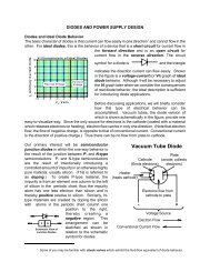
The basic idea of feedback is straightforward: the results of some process are monitored, 

compared to a goal, and the input is adjusted based on the difference between the results 

and goal. This can be represented diagrammatically as follows: 

Input 

(goal) 

Comparison 

Point 

Process 

Results 

Monitor 

Generalized diagram of Feedback 

In fact, in everyday life, we can identify many examples of feedback: keeping our car on 

the road when driving, behavior modification techniques, etc. Of course, we will restrict our 

attention to electronic implementation of feedback. From that perspective, the signals to 

monitor and control may be voltage, current, or power. As we have done previously, we 

will further restrict ourselves to cases of voltage feedback. 

Amplifier-based voltage-feedback systems are basically as indicated below. (The set of +’s 

and -‘s indicate the standard sign convention for summing voltages in the input loop.) From 

the diagram, we can derive the relation between the input and output, also as indicated 

below. 

Feedback Amplifier Analysis : 

Voltage Feedback Amplifier System 

V = V + β V (KVL input loop analysis) 

V = AV = A(V + β V ) (Based on no - load output) 

V 

V 

it in o 

o it in o 

o 

in 

A 

= = G (Voltage - feedback 

1 - βA 

amplifier relation) 

+ + 

V it 

R oa 

V in 

R 

V o 

ia 

- - 

A*V it 

+ - 

ßV o 

ß 

V o 

DISCUSSION OF THE FEEDBACK RELATION 

Prior to making use of feedback, we need to examine the feedback relation for G in some 

detail. First, the factor represented by $ can be many things: another amplifier, a filter, a 

phase-shift network, a voltage divider, etc. However, we will represent its effect as the

Feedback Amplifiers GEORGIA STATE UNIVERSITY Page 2 of 8 

mathematical factor $ which in general is a complex number. Likewise, the amplifier 

may introduce phase-shift, and / or frequency dependence; thus A in general also is a 

complex number. The product A$, appearing in the denominator of the feedback 

relation is therefore in general a complex number. 

From our previous discussion of complex number algebra, we know that the magnitude of 

a product is the product of the magnitudes, and that the phase angle of a product is the 

sum of the phase angles. Thus, for emphasis, we can express A$ as 

Aβ =Aβ and φ = φ + φ Recall also that inversion (multiplication by -1) is the same 

Aβ A β. 

as a 180° phase shift, and that 0°, 360°, ...Nx360° all describe the in-phase condition. 

From this, we can identify two basic cases of the expression for G to examine further: 

1. A β > 0 ( Positive real number) 

means φA 

+ φβ 

= 0 , 360 ,..., n * 360 

Positive Feedback 

! ! ! 

2. A β < 0 ( Negative real number) 

means φA 

+ φβ 

= 180 , 540 , ... 180 +n * 360 

Negative Feedback 

! ! ! ! 

Of course, there are in-between cases where A$ is a complex number. However, these 

two cases listed above, where the A$ product is a real number, are very inportant for 

several reasons, some of which will be discussed below. 

Positive Feedback. Positive feedback is the situation where the adjustment is applied to 

reinforce (or add to) the difference between the goal and the results. Obviously. This 

adjustment moves the results even farther from the goal and is undesirable in most cases. 

(In psychology and behavior modification, the term “positive feedback” is often used; 

however, it matches our description only from the view that the feedback moves the results 

further away from an undesirable goal.) For example, in driving a car, one aim is to keep 

the car along the chosen path. This is accomplished by monitoring the actual path in 

comparison to that desired and applying an adjustment opposite to the difference. If the 

adjustment reinforced the difference, as would be the case with positive feedback, the path 

would become even more in error—perhaps leading to the ditch! 

Nevertheless, positive feedback in electronics has at least one clear application, that of 

producing oscillators. For example, consider the case A$ = 1, which makes the 

denominator 1 - A$ = 0, and G infinite! A physical interpretation of this condition is that $ 

represents signal reduction in the feedback path while A represents restoration. That is, 

if A exactly restores that which was lost, then the feedback creates a self-sustaining signal 

(as long as it is started in the first place). If A > 1/$, the signal grows until limited by some 

other factor (power supply, etc.). In the case of A$ $1, no “input” in needed and the 

feedback amplifier circuit becomes as shown in the circuit below.


Notice that V it = $V o and that the algebra 

seems contradictory if we write 

V = AβV when A β > 1. 

o 

o 

Voltage Feedback Amplifier System, 

Oscillator Configuration 

The condition for self-sustaining signals 

(or oscillation, called the Barkhausen 

Criterion, is 

A β = 1 , 

+ 

- 

+ 

- 

V it 

R ia 

R oa 

A*V it 

V o 

or A β = 1 , 

and φ + φ = 0, 360, ..., n* 360. 

A 

β 

! ! ! 

ßV o 

ß 

V o 

For oscillators, a main application of 

positive feedback, $ is designed to have 

a frequency dependence so that A β → 1 @ f o. 

For example, consider the phase-shift 

oscillator sketched below. The amplifier is in the op-amp inverting configuration. 

Therefore, N A = 180° and at f o it is also 

necessary that N $ = 180°. An a.c. circuit 

Phase Shift Oscillator 

analysis of the RC network 

R 

(straightforward, but tedious) yields: 

f 

V2 

1 

β = = 

V1 

5 

⎡ 

1 

⎤ 

1 

1 - + j ⎢ - 6⎥ 

2 2 

( ωRC) ⎢( ω ) ⎥ωRC 

⎣ RC ⎦ 

R i 

C C C 

V 1 (= V out ) 

R R R 

V 2 (=ßV o ) 

V o / V i is purely real when the imaginary 

term in square brackets is zero, or when 

(TRC) 2 = 1/6. Also, when this condition is 

Vo 

1 1 

satisfied, β = = = - . Thus, for the phase-shift oscillator shown above, 

V 1 - 5⋅6 + j[0] 29 

i 

1 

the Barkhausen criterion is satisfied at ω0 = 2πf 0 = if A ≤- 29 ( A ≥29). 

6RC 

Negative Feedback. Negative feedback is the case more generally applied. For the 

example of driving described above, adjustment of the car’s direction opposite to the 

deviation corrects the deviation and is an example of negative feedback. Many 

applications of negative feedback are in control-system design (guidance systems, voltage 

regulators, etc.) However, because the phase shift of electronic (and mechanical devices) 

is a function of frequency, usually increasing with increasing frequency, it is necessary that 

the design prevent unintentional occurrence of the Barkhausen condition. (You wouldn’t 

like being a passenger on a plane where the autopilot exhibited this condition!) In fact, the 

central problem of control-system design is to provide quick response while preventing 

occurrence of the Barkhausen condition.


Several circuits we have already considered employ negative feedback. Of these, we will 

examine two in more detail, the non-inverting amplifier configuration with operational 

amplifiers and our transistor amplifier. In addition, we will examine a voltage regulator 

system using negative feedback. 

Negative Feedback and the Non-inverting Op-Amp Circuit. Shown below is a re-sketch 

of this amplifying circuit emphasizing the connection between the output and the input. 

The main new element in the analysis is 

retaining A as a finite value. (R in is still 

taken as large enough to make I amp ~ 0.) 

Analysis of the circuit yields: 

V + = Vin 

⎛ R2 

⎞ 

V - = Vout 

⎜ ⎟ 

⎝R 1+ R2 

⎠ 

⎛ VoutR2 

⎞ 

out + - ⎜ in ⎟ 

⎝ 1 2 ⎠ 

Vout 

A 

= = G 

Vin 

1 + AR 2 

(R + R ) 

1 2 

Non-Inverting Op-Amp 

V 

V out = A(V + - V - ) 

in 

A 

V - = V out R 2 /(R 1 + R 2 ) 

R 1 

R 2 

V = A(V - V ) = A V - R + R 

⎛ ⎞ 

Since this expression is different from that obtained previously, but the previous derivation 

used the approximation A →∞, 

we should examine this new result for correspondence to 

the earlier one. Doing so gives the expressions: 

⎛ 

⎞ 

lim ⎛ V ⎞ ⎜ A ⎟ ⎜ 1 ⎟ R + R R 

→∞⎜ ⎟= lim 

→∞⎜ ⎟= lim 

→∞⎜ 

⎟= = 1 + 

A 

⎝ V A A 

⎠ ⎜1 + 

AR2 ⎟ 1 R2 

⎜ R R 

⎟ 

⎝ (R 1 + R 2) + 

⎠ ⎝ A (R 1 + R 2) 

⎠ 

out 1 2 1 

in 2 2 

Things are OK since this is the same result as before. Also, by examination of the 

R2 

expression for G, it is evident that A β = -A for this circuit. 

R + R 

1 2 

Example 1: Calculate the actual voltage “Gain” of a circuit in the non-inverting op-amp 

configuration when A = 50 and R 1 / R 2 = 99. 

50 50 1 

Solution: Using the result above, we get G = = = 33 . 

R2 

50 

1 + 

3 

1 + 50 

R + 99R 100 

2 2 

Example 2: Calculate the minimum value of A to make the actual voltage “Gain” of a 

circuit in the non-inverting op-amp configuration at least 90% of the “ideal value” 

when R 1 / R 2 = 99.


Solution: The “ideal” value is G = 1 + R 1 / R 2 = 1 + 99 = 100. So, the question becomes 

that of finding the value of A making G $90. By algebraic rearrangement, we can 

G 

solve (or re-derive) the expression above for A: A = 

. 

R 

Thus the value 

2 

1 - G R + R 

needed is A $ 90 / (1 - 0.9) = 900. 

1 2 

Feedback Voltage Regulator: Using feedback to accomplish the voltage regulation 

function can be envisioned as in the diagram. The concepts are a monitor of the actual 

output which compares it to the reference (desired behavior) and controls the “adjust” 

element. An actual implementation of such a circuit (for positive voltages) using an 

amplifier and an NPN transistor is shown beside the diagram. 

Conceptual Feedback Voltage Regulator 

Feedback Voltage Regulator 

(Positive Voltages) 

Unreg. Input 

Adjust 

Output 

+ Unreg. in 

V out 

R 1 

Reference 

Monitor 

R 2 

V ref 

V = V 

+ ref 

⎛ R2 

⎞ 

V - = Vout 

⎜ ⎟ 

⎝R 1+ R2 

⎠ 

V oa = V b = A(V + - V - ) 

V = V -0.7 = A(V - V )-0.7 

out b + - 

⎛ VoutR2 

⎞ 

V out = A⎜V ref - ⎟-0.7 

⎝ R 1+ R2 

⎠ 

⎛ ⎞ ⎛ ⎞ 

⎜ ⎟ ⎜ ⎟ 

⎜ 

A 

⎟ ⎜ 

0.7 

V ⎟ 

out = Vref 

- 

⎜ R2 ⎟ ⎜ R2 

⎟ 

⎜ 

1 +A 

⎟ ⎜ 

1 +A 

⎟ 

⎝ R 1+ R2 ⎠ ⎝ R 1+ R2 

⎠ 

Analysis of the circuit is as follows: 

The second term in the analysis, resulting 

from the base-emitter voltage of the 

transistor, is insignificant in most cases. 

Specifically, the denominator is the same in 

both terms; the numerator of the first is Avref , 

while that of the second is 0.7. In cases 

where A is large, the first will clearly be 

dominant. Therefore, except for testing to 

see how important the second term might 

be, we will consider only the first term. 

One other aspect of the analysis is the 

similarity with the result obtained above for 

the non-inverting op-amp configuration. 

Actually, this is not accidental since the voltage regulator circuit can be rearranged as 

shown below to emphasize its close relationship to the non-inverting amplifier circuit.


In fact, the voltage regulator is the noninverting 

amplifier with a transistor in the 

output. In addition, V ref is simply the “input.” 

This correspondence provides another 

insight we will use later. 

Returning now to the voltage regulator 

analysis above, we see that the main term 

in the expression is 

Voltage Regulator Related to 

Non-Inverting Op-Amp 

V ref 

+ Unreg. in 

V 

R out 

1 

R 2 

⎛ 

⎞ 

⎜ 

⎟ 

⎜ 

A 

V ⎟ 

out = Vref 

which is the 

⎜ R2 

⎟ 

⎜ 

1 + A 

⎟ 

⎝ R 1 + R 2 ⎠ 

same as that for the non-inverting amplifier. 

By the same algebra, for large A, the result 

for the output is simply V out = V ref (1 + R 2 / R 1 ). In other words, the output is simply the 

“amplified” version of the reference. 

Finally, it is important to point out that the role of the reference voltage is to provide the 

definition of “steady.” It is not necessary that the reference voltage be equal to that sought 

by the regulator since the output is multiplied by the factor determined by the resistors as 

described above. The purpose of the regulator is to provide an output with voltage steady 

as possible, but it can do so only with by comparison with a standard, or reference, defining 

“steady.” This is a role played often by zener diodes in electronic voltage regulators. 

Example 3: Calculate the error in ignoring the “second” term and the actual value of A in 

the voltage regulator analysis for the case A = 25, V ref = 1.25V, and R 1 / R 2 = 9. 

Solution: The “ideal” value is V o = V ref ( 1 + R 1 / R 2 ) = 12.5V. The actual value using the 

numbers given is V o = 1.25 x25 / (1 + 25/10) - 0.7 / (1 +25 / 10) = 8.9V. So the error 

is ~ 3.6 V, or about 29%. In fact, increasing A to 250 yields V out ~ 12v, reducing the 

error to a much smaller amount. 

Negative Feedback in Our Transistor Amplifier. As you might suspect by now, the very 

simple relation derived for amplification of our simple transistor amplifier circuit suggests 

the presence of some effect such as feedback. In fact negative feedback plays a direct 

and important role in the circuit. We can see this by revisiting the amplifying portion of the 

circuit as sketched below. The one thing we need to modify is the absolutely constant 

difference between base and emitter voltages. We knew this was not strictly true earlier, 

but must make use of the fact that the base-emitter junction can be better approximated 

as a resistance h ie ( nominal values are ~1k). Thus, while the base-emitter junction is 

conducting, V be ~ h ie I b , and V be is not exactly constant


In the circuit, the voltages expressed in lower case 

are to be understood as the changing components 

only. Recall that the circuit is an a.c. amplifier only; 

thus only voltage changes are important. 

Transistor Amplifier for 

Feedback Identification 

Analysis of the circuit is as follows: 

v in = vb 

v o = v c = -i c Rc 

vR o e 

v e = i c R e = - 

Rc 

v b - v 

i c = hfei b = h fe 

h 

ie 

e 

v - v h ⎛ v R 

v o =- Rch fe = - Rc ⎜v in + 

hie hie ⎝ Rc 

⎛ hfe 

⎞ 

⎜- Rc 

⎟ 

vo 

⎝ hie 

⎠ (- Rchfe) 

A = = = 

vin ⎛ hfeRe 

⎞ ( h ie + hfeRe 

) 

⎜1 + ⎟ 

⎝ h ie ⎠ 

b e fe o e 

⎞ 

⎟ 

⎠ 

v b 

= v in 

h ie 

R c 

v c = -i c R c 

v e = i c R e 

The positive sign of the second term in the denominator indicates the negative feedback. 

Our approach actually used the approximation h ie = 0, which yields our result, that the 

amplification A = -R c / R e . This expression also shows the appropriate version for A in the 

case R e becomes zero: A = -R c h fe /h ie , an result heavily dependent on electrical parameters 

of the transistor. 

Comments on Use of Negative Feedback in General with Amplifiers. The insight from 

comparing the voltage regulator to the non-inverting amplifier circuit will now be useful in 

understanding the value of negative feedback in general use with amplifier design. 

Specifically, feedback in general compares the result of a “process” to a “goal” and makes 

“adjustments” based on the difference. Negative feedback makes the adjustments in a 

way tending to reduce the difference or “error.” 

In general-purpose amplifiers, the input is the “reference” to which the output is to be 

compared. Thus, negative feedback has the property of reducing amplifier-induced 

distortion. 

Effect of feedback on Input and Output Resistances. 

Our final task will be to examine the correspondence between the characteristics of the 

basic amplifier, the feedback connection, and the effective input and output resistances of 

the circuit including feedback. The “standard” circuit from above is copied below for this 

purpose. 

Effective Input Resistance. As before, the approach will be based on the Thevenin 

concept. For the input resistance, we will “apply” an input voltage, and seek a relation 

between it and the resulting current so that R in = V in / I in . By examination of the circuit, we 

can see the following: 

R e 

+V s


V V GV 1 V 

I in = = = = 

R AR AR (1- Aβ 

) R 

Vin 

R in = = (1- Aβ 

) Ria 

I 

it o in in 

ia ia ia ia 

in 

Thus, for positive feedback, where 1-A$ 

is less than 1 and may approach zero, the 

input resistance is less than that of the 

basic amplifier. In contrast, for negative 

feedback, where 1-A$ is positive and 

greater than 1, the effective input resistance 

) 

) 

V = AV = GV 

out open it in 

AV 

it 

I out = 

short R oa 

AVin 

Vout ) 

open GV in (1- A β ) Roa 

R out = = = = 

I out ) AVit 

AVin 

(1- A β ) 

short 

R R 

oa 

Voltage Feedback Amplifier System 

+ 

I in 

+ 

V it 

R oa 

V in 

R 

V o 

ia 

- - 

A*V it 

+ - 

is greater than that of the basic amplifier. Thus, in terms of a general-purpose voltage 

amplifier, negative feedback enhances the input resistance. 

Effective Output Resistance. Also as before, our approach will be to use the Thevenin 

perspective. Specifically, we will seek the ratio of the open-circuit output voltage to the 

short-circuit output current. 

However, the case when the output is short-circuited must be examined more carefully 

since V o = 0 under those circumstances. Specifically, when V o = 0, $V o = 0, also and 

V it = V in . So, 

oa 

ßV o 

ß 

V o 

For positive feedback, where 1-A$ will be less than 1, and may approach zero, the 

effective output resistance is greater than that of the basic amplifier. On the other hand, 

for negative feedback, where 1-A$ will be greater than 1, the output resistance is less than 

that of the basic amplifier. In summary, for a general-purpose voltage amplifier, 

negative feedback improves the effective output resistance. 

Conclusions: Both positive and negative feedback have useful applications. In particular, 

negative feedback has a wide range of applications in control-system technology. 

Moreover, negative feedback provides improved characteristics of general-purpose 

amplifiers: distortion is reduced, the input resistance is increased, and the output 

resistance is decreased.

C:\My Documents\feedback.wpd - Georgia State University

Create successful ePaper yourself

Delete template?

Save as template?