Magnetic Field Uniformity of Helmholtz Coils and Cosine θ Coils
Magnetic Field Uniformity of Helmholtz Coils and Cosine θ Coils
Magnetic Field Uniformity of Helmholtz Coils and Cosine θ Coils

Create successful ePaper yourself
Turn your PDF publications into a flip-book with our unique Google optimized e-Paper software.
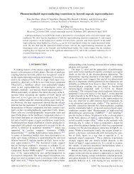
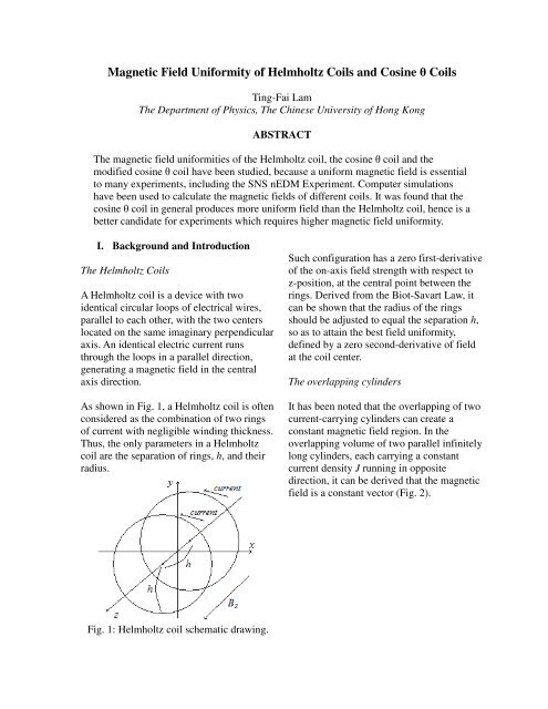
<strong>Magnetic</strong> <strong>Field</strong> <strong>Uniformity</strong> <strong>of</strong> <strong>Helmholtz</strong> <strong>Coils</strong> <strong>and</strong> <strong>Cosine</strong> θ <strong>Coils</strong><br />
Ting-Fai Lam<br />
The Department <strong>of</strong> Physics, The Chinese University <strong>of</strong> Hong Kong<br />
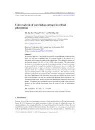
ABSTRACT<br />
The magnetic field uniformities <strong>of</strong> the <strong>Helmholtz</strong> coil, the cosine θ coil <strong>and</strong> the<br />
modified cosine θ coil have been studied, because a uniform magnetic field is essential<br />
to many experiments, including the SNS nEDM Experiment. Computer simulations<br />
have been used to calculate the magnetic fields <strong>of</strong> different coils. It was found that the<br />
cosine θ coil in general produces more uniform field than the <strong>Helmholtz</strong> coil, hence is a<br />
better c<strong>and</strong>idate for experiments which requires higher magnetic field uniformity.<br />
I. Background <strong>and</strong> Introduction<br />
The <strong>Helmholtz</strong> <strong>Coils</strong><br />
A <strong>Helmholtz</strong> coil is a device with two<br />
identical circular loops <strong>of</strong> electrical wires,<br />
parallel to each other, with the two centers<br />
located on the same imaginary perpendicular<br />
axis. An identical electric current runs<br />
through the loops in a parallel direction,<br />
generating a magnetic field in the central<br />
axis direction.<br />
As shown in Fig. 1, a <strong>Helmholtz</strong> coil is <strong>of</strong>ten<br />
considered as the combination <strong>of</strong> two rings<br />
<strong>of</strong> current with negligible winding thickness.<br />
Thus, the only parameters in a <strong>Helmholtz</strong><br />
coil are the separation <strong>of</strong> rings, h, <strong>and</strong> their<br />
radius.<br />
Such configuration has a zero first-derivative<br />
<strong>of</strong> the on-axis field strength with respect to<br />
z-position, at the central point between the<br />
rings. Derived from the Biot-Savart Law, it<br />
can be shown that the radius <strong>of</strong> the rings<br />
should be adjusted to equal the separation h,<br />
so as to attain the best field uniformity,<br />
defined by a zero second-derivative <strong>of</strong> field<br />
at the coil center.<br />
The overlapping cylinders<br />
It has been noted that the overlapping <strong>of</strong> two<br />
current-carrying cylinders can create a<br />
constant magnetic field region. In the<br />
overlapping volume <strong>of</strong> two parallel infinitely<br />
long cylinders, each carrying a constant<br />
current density J running in opposite<br />
direction, it can be derived that the magnetic<br />
field is a constant vector (Fig. 2).<br />
Fig. 1: <strong>Helmholtz</strong> coil schematic drawing.
Fig. 2: Constant B-field generated by two<br />
overlapping current-carrying cylinders.<br />
The pro<strong>of</strong> is as follow. Consider the volume<br />
in the cylinder carrying a current density J,<br />
whose axis coincides with the z-axis, the B-<br />
field inside should be:<br />
Fig. 3: Overlapping cylinders for small d.<br />
Hence, it is also possible to represent such<br />
configuration with only one cylinder,<br />
carrying a surface current whose density σ(θ)<br />
is proportional to cos θ, as shown below:<br />
... Eq. (1).<br />
Similarly, inside another cylinder with<br />
current density –J, whose axis is parallel but<br />
displaced towards –y direction by d, the B-<br />
field is:<br />
... Eq. (2).<br />
Fig. 4: The “idealized” cosine θ setup.<br />
A vector addition will show:<br />
The <strong>Cosine</strong> θ coils<br />
... Eq. (3).<br />
In the limit when axial displacement d<br />
approaches 0, only two “new moon shaped”<br />
channels would still contain a current. The<br />
amount <strong>of</strong> current in the infinitesimal<br />
volume is proportional to cos θ, which is<br />
defined as:<br />
Fig. 5: <strong>Cosine</strong> θ coils schematic drawing. [1]<br />
The cosine θ coil in Fig. 5 can be considered
as a practical approximation to the<br />
arrangement in Fig. 4. In order to reproduce<br />
the density distribution σ(θ) = σ 0 cos θ, the<br />
wires are wound on the coil such that the x-<br />
axis projections <strong>of</strong> all windings are<br />
uniformly distributed. The angle θ <strong>of</strong> the<br />
windings can be expressed as: [2] ... Eq. (4),<br />
where J = 1 ... N/2, <strong>and</strong> K = 0.<br />
The cosine θ coil replaces the continuous<br />
current densities with a total <strong>of</strong> N discrete<br />
wires, <strong>and</strong> also the infinitely long cylinder<br />
with a finite L/R ratio, where L is the<br />
cylindrical length <strong>of</strong> the coil <strong>and</strong> R is the<br />
radius. The effects <strong>of</strong> the two approximations<br />
will be investigated.<br />
Modified cosine θ coils<br />
A simple cosine θ coil has a field gradient. In<br />
order to produce more uniform magnetic<br />
field, it is possible to combine two coils with<br />
different number <strong>of</strong> turns, N, to partially<br />
cancel the gradient. [3] The combination <strong>of</strong> a<br />
main coil <strong>and</strong> a secondary coil, having<br />
different number N, <strong>and</strong> running the currents<br />
in opposite directions, will be called a<br />
“modified cosine θ coil”.<br />
The uniformity <strong>of</strong> field is reflected by the<br />
fractional change, which is independent <strong>of</strong><br />
the actual value <strong>of</strong> the current running in the<br />
coil. The modified cosine θ coils introduce<br />
the following two parameters, namely N 2 in<br />
the secondary coil, <strong>and</strong> the current ratio I 2 /I,<br />
where I <strong>and</strong> I 2 are the currents in the main<br />
<strong>and</strong> secondary coils.<br />
<strong>Magnetic</strong> field uniformity <strong>and</strong> fractional<br />
change<br />
<strong>Magnetic</strong> field uniformity is represented by<br />
the fractional change <strong>of</strong> field relative to the<br />
field at the origin. This is a function <strong>of</strong><br />
position, explicitly:<br />
... Eq. (5).<br />
The closer this value is to zero, the more<br />
uniform the field is. Similar definitions hold<br />
for y, z field components, <strong>and</strong> y, z position<br />
dependence.<br />
II. Method<br />
Computer simulations<br />
A Fortran program <strong>and</strong> a Mathematica<br />
program were written to numerically<br />
integrate the Biot-Savart Law, hence<br />
calculate the resultant B-field generated by a<br />
coil.<br />
Because the Mathematica program allows<br />
flexible numerical plotting, it was used to<br />
investigate the field dependence on position.<br />
Other than absolute values <strong>of</strong> magnetic field,<br />
the program was used to calculate the<br />
fractional change <strong>of</strong> field as a function <strong>of</strong><br />
position, defined as in Eq. (5).<br />
Comparison <strong>of</strong> various coils<br />
<strong>Field</strong> dependence on position cannot be<br />
compared in all 3 dimensions, owing to the<br />
different orientations <strong>of</strong> the <strong>Helmholtz</strong> <strong>and</strong><br />
the cosine θ coils.<br />
To compare the cosine θ coil with the<br />
<strong>Helmholtz</strong> coil, one “primary” axis is<br />
identified. Even if the field in the coil<br />
volume is not “unidirectional”, it is clear that<br />
the <strong>Helmholtz</strong> coil generates field primarily<br />
towards its z-axis, while the cosine θ coil<br />
generates towards z-axis. Such axis will be<br />
addressed the “primary” axis <strong>of</strong> each coil. In<br />
other words, the B z (z) for <strong>Helmholtz</strong> coil <strong>and</strong><br />
B x (x) for cosine θ coil will be considered in
every comparison plot.<br />
along the x-axis (1.0 meter full range).<br />
The cosine θ coil radius R is always set to be<br />
h/2, where h is both the separation <strong>and</strong> radius<br />
<strong>of</strong> <strong>Helmholtz</strong> coil. The magnetic field is<br />
generated in x direction for <strong>Helmholtz</strong> coil,<br />
while in z direction for cosine θ coil. This<br />
setting would allow the lengths <strong>of</strong> the<br />
primary axes to be the equal for both coils.<br />
For the cosine θ coil, the two parameters N<br />
<strong>and</strong> L/R ratio are varied to see the effects on<br />
the field uniformity. Also the <strong>Helmholtz</strong> coil,<br />
both the simple <strong>and</strong> modified cosine θ coils<br />
are compared.<br />
Fig. 7: <strong>Helmholtz</strong> coil field fractional change<br />
along the x-axis (0.2 meter = 20% zoom-in).<br />
III. Results <strong>and</strong> Discussion<br />
<strong>Field</strong> generated by a <strong>Helmholtz</strong> coil<br />
Fig. 6 to 9 show the B z fractional change<br />
along the 3 axes for the <strong>Helmholtz</strong> coil. The<br />
first pair <strong>of</strong> plots are the dependence along<br />
the x-axis, with the first showing the whole<br />
0.5-meter range, while the second showing<br />
only 0.2-meter zoom-in.<br />
The next pair are for z dependence. Because<br />
x <strong>and</strong> y directions are symmetric for the coil,<br />
the y-axis plots are omitted.<br />
Fig. 8: <strong>Helmholtz</strong> coil field fractional change<br />
along the z-axis (0.5 meter full range). Note<br />
it is the “primary” axis.<br />
The specifications are:<br />
h = 0.5 meters,<br />
where h is both the radius <strong>and</strong> separation.<br />
Fig. 9: <strong>Helmholtz</strong> coil field fractional change<br />
along the z-axis (0.2 meter = 40% zoom-in).<br />
Note it is the “primary” axis.<br />
Fig. 6: <strong>Helmholtz</strong> coil field fractional change<br />
From the above plots, it is found that the<br />
fractional change takes a “saddle-shaped”<br />
positional dependence. As expected, it has a
stationary point at the center, which is also<br />
the global maximum.<br />
Some characteristics are the fractional<br />
change plots do not change in shape upon<br />
zooming in. The uniformity <strong>of</strong> the primary<br />
axis is relatively worse than the other (x- <strong>and</strong><br />
y-) axes.<br />
<strong>Field</strong> generated by a cosine θ coil<br />
Fig. 10 to 15 show the B x fractional change<br />
along the 3 axes for the cosine θ coil. The<br />
first pair <strong>of</strong> plots are the dependence along<br />
the x-axis, with full range <strong>and</strong> zoom-in<br />
respectively. The remaining 2 pairs are for y<br />
<strong>and</strong> z dependence.<br />
Fig. 11: <strong>Cosine</strong> θ coil field fractional change<br />
along the x-axis (0.2 meter = 40% zoom-in).<br />
Note it is the “primary” axis.<br />
The specifications are:<br />
R = 0.25 meters, L = 1 meter, L/R = 4.0,<br />
where R is the radius <strong>and</strong> L is the cylindrical<br />
length.<br />
N = 22.<br />
Fig. 12: <strong>Cosine</strong> θ coil field fractional change<br />
along the y-axis (0.5 meter full range).<br />
Fig. 10: <strong>Cosine</strong> θ coil field fractional change<br />
along the x-axis (0.5 meter full range). Note<br />
it is the “primary” axis.<br />
Fig. 13: <strong>Cosine</strong> θ coil field fractional change<br />
along the y-axis (0.2 meter = 40% zoom-in).
sections, explicitly stated as follow.<br />
For <strong>Helmholtz</strong> coil:<br />
h = 0.5 meters.<br />
B z (z) is observed.<br />
For all cosine θ coils:<br />
R = 0.25 meters, L = 1 meter, L/R = 4.0.<br />
B x (x) is observed.<br />
Fig. 14: <strong>Cosine</strong> θ coil field fractional change<br />
along the z-axis (1.0 meter full range).<br />
<strong>Helmholtz</strong><br />
Cosθ N=40<br />
Cosθ N=22<br />
Cosθ N=12<br />
Cosθ N=8<br />
Fig. 16: Taking N as the parameter, field<br />
fractional change plot <strong>of</strong> various coils along<br />
the primary axis (0.5 meter full range).<br />
Fig. 15: <strong>Cosine</strong> θ coil field fractional change<br />
along the z-axis (0.2 meter = 20% zoom-in).<br />
On the primary x-axis, the fractional change<br />
takes an “m-shaped” positional dependence,<br />
with the center being a local minimum.<br />
Both the y <strong>and</strong> z dependence has a saddle<br />
shape. Same as the <strong>Helmholtz</strong> coil, plot <strong>of</strong> z<br />
dependence retains a similar shape upon<br />
zooming. The uniformity along y axis, on the<br />
other h<strong>and</strong>, clearly worsens only near the<br />
edges.<br />
Comparison for various N<br />
N is taken as a parameter here. The primary<br />
component field fractional change along the<br />
primary axis for various cosine θ coils, <strong>and</strong><br />
the <strong>Helmholtz</strong> coil, are plotted together in<br />
Fig. 16 <strong>and</strong> 17.<br />
The specifications are the same as above<br />
Cosθ N=8<br />
Cosθ N=12<br />
Cosθ N=22<br />
Cosθ N=40<br />
<strong>Helmholtz</strong><br />
Fig. 17: Taking N as the parameter, field<br />
fractional change plot <strong>of</strong> various coils along<br />
the primary axis (0.2 meter = 40% zoom-in).<br />
Since the field uniformity is better when the<br />
fractional change is close to zero, N = 40 has<br />
the best uniformity while N = 8 has the<br />
worst. It verifies the expectation that a<br />
greater N produces better uniformity,<br />
because it better compensates the<br />
approximation to the continuous current<br />
density (Fig. 4) by more lines <strong>of</strong> current.<br />
For the particular length specifications used
here, N = 40 approximately corresponds to<br />
the <strong>Helmholtz</strong> coil uniformity considering<br />
the full range, while N = 22 approximately<br />
corresponds to that in the zoom-in.<br />
Comparison for various L/R ratios<br />
L/R ratio is taken as a parameter here. The<br />
primary component field fractional change<br />
along the primary axis for various cosine θ<br />
coils, <strong>and</strong> the <strong>Helmholtz</strong> coil, are plotted<br />
together in Fig. 18 <strong>and</strong> 19.<br />
The specifications are the same as above<br />
sections, explicitly stated as follow.<br />
For <strong>Helmholtz</strong> coil:<br />
h = 0.5 meters.<br />
B z (z) is observed.<br />
For all cosine θ coils:<br />
R = 0.25 meters, N = 22.<br />
B x (x) is observed.<br />
Cosθ L/R=2.4<br />
Cosθ L/R=3.2<br />
Cosθ L/R=4.0<br />
Fig. 19: Taking L/R ratio as the parameter,<br />
field fractional change plot <strong>of</strong> various coils<br />
along the primary axis (0.2 meter = 40%<br />
zoom-in).<br />
From the plots above, L/R = 4.8 has the best<br />
field uniformity, while L/R = 2.4 has the<br />
worst. It can be justified in terms <strong>of</strong><br />
approximation to the ideal case, where L/R is<br />
infinity. Referring to Fig. 5, it is also noted<br />
that the “edge current” is less effective when<br />
L/R is large.<br />
Modified cosine θ coils<br />
<strong>Cosine</strong> θ coil can be modified by combining<br />
another cosine θ coil with different N, which<br />
runs in opposite directions. The number N 2<br />
<strong>and</strong> the current ratio I 2 /I for the secondary<br />
current can be determined by trial-<strong>and</strong>-error.<br />
The specifications for the Fig. 20 to 25 are:<br />
For both coil:<br />
R = 0.25 meters, L = 1 meter, L/R = 4.0.<br />
For main coil:<br />
N = 22.<br />
For secondary coil:<br />
N 2 = 8, I 2 /I = –0.75.<br />
Cosθ L/R=4.8<br />
<strong>Helmholtz</strong><br />
Fig. 18: Taking L/R ratio as the parameter,<br />
field fractional change plot <strong>of</strong> various coils<br />
along the primary axis (0.5 meter full range).<br />
Modified<br />
Simple<br />
Cosθ L/R=2.4<br />
Cosθ L/R=3.2<br />
Cosθ L/R=4.0<br />
Cosθ L/R=4.8<br />
Fig. 20: Simple <strong>and</strong> modified cosine θ coil<br />
field fractional change along the x-axis (0.5<br />
meter full range). Note it is the “primary”<br />
axis.<br />
<strong>Helmholtz</strong>
Modified<br />
Simple<br />
Simple<br />
Modified<br />
Fig. 21: Simple <strong>and</strong> modified cosine θ coil<br />
field fractional change along the x-axis (0.2<br />
meter = 40% zoom-in). Note it is the<br />
“primary” axis.<br />
Fig. 24: Simple <strong>and</strong> modified cosine θ coil<br />
field fractional change along the z-axis (1.0<br />
meter full range).<br />
Modified<br />
Simple<br />
Modified<br />
Simple<br />
Fig. 22: Simple <strong>and</strong> modified cosine θ coil<br />
field fractional change along the y-axis (0.5<br />
meter full range).<br />
Modified<br />
Simple<br />
Fig. 23: Simple <strong>and</strong> modified cosine θ coil<br />
field fractional change along the y-axis (0.2<br />
meter = 40% zoom-in).<br />
Fig. 25: Simple <strong>and</strong> modified cosine θ coil<br />
field fractional change along the z-axis (0.2<br />
meter = 20% zoom-in).<br />
The plots show that a secondary coil can<br />
effectively reduce the field gradient in the<br />
central region <strong>of</strong> the coil. For the 0.2-meter<br />
zoom-in region, the uniformity is improved<br />
by more than 25 times <strong>and</strong> about 7 times, for<br />
the x-axis <strong>and</strong> the y-axis respectively.<br />
The uniformity <strong>of</strong> a modified cosine θ coil is<br />
not as good for the edge regions <strong>of</strong> each axis.<br />
Also the uniformity on z-axis is totally<br />
unaffected, as seen from Fig. 24 <strong>and</strong> 25.<br />
IV. Conclusions<br />
To conclude, the magnetic field uniformities<br />
<strong>of</strong> the <strong>Helmholtz</strong> coil, various simple cosine<br />
θ coil <strong>and</strong> modified cosine θ coil, which are<br />
represented by the fractional change <strong>of</strong> field
elative to the coil origin, have been<br />
observed <strong>and</strong> compared through simulation.<br />
It was found that the cosine θ coil is a better<br />
c<strong>and</strong>idate than the <strong>Helmholtz</strong> coil to<br />
generate a uniform magnetic field, given<br />
suitable number <strong>of</strong> turns N, length-to-radius<br />
ratio L/R, <strong>and</strong> secondary coil modification if<br />
possible.<br />
V. Acknowledgments<br />
I gratefully acknowledge the help <strong>and</strong><br />
beaconing advice from Jen-Chieh Peng <strong>and</strong><br />
Ping-Han Chu. This work is completed<br />
under the REU program, which is supported<br />
by National Science Foundation Grant PHY-<br />
0647885.<br />
VI. Footnotes, Endnotes <strong>and</strong><br />
References<br />
[1] B. Plaster, talk presented at the SNS<br />
nEDM Experiment Collaboration Meeting<br />
(October 2006).<br />
[2] S. Balascuta <strong>and</strong> R. Alarcon, talk<br />
presented at the SNS nEDM Experiment<br />
Collaboration Meeting (June 2009).<br />
[3] R. Schmid, talk presented at the SNS<br />
nEDM Experiment Collaboration Meeting<br />
(March 2006).