Constructing soluble quantum spin models - Department of Physics ...
Constructing soluble quantum spin models - Department of Physics ...
Constructing soluble quantum spin models - Department of Physics ...

You also want an ePaper? Increase the reach of your titles
YUMPU automatically turns print PDFs into web optimized ePapers that Google loves.
Nuclear <strong>Physics</strong> B 666 [FS] (2003) 337–360<br />
www.elsevier.com/locate/npe<br />
<strong>Constructing</strong> <strong>soluble</strong> <strong>quantum</strong> <strong>spin</strong> <strong>models</strong><br />
H.Y. Shik a ,Y.Q.Li a,b ,H.Q.Lin a<br />
a <strong>Department</strong> <strong>of</strong> <strong>Physics</strong>, the Chinese University <strong>of</strong> Hong Kong, Hong Kong, PR China<br />
b Zhejiang Institute <strong>of</strong> Modern <strong>Physics</strong>, Zhejiang University, PR China<br />
Received 31 October 2002; received in revised form 28 April 2003; accepted 27 May 2003<br />
Abstract<br />
By applying the bond operator method, we construct several <strong>soluble</strong> <strong>quantum</strong> <strong>spin</strong> <strong>models</strong> in<br />
two and three dimensions. We first generalize the <strong>spin</strong>-1/2 bond operators developed by Sachdev<br />
and Bhatt [Phys. Rev. B 41 (1990) 9323] to <strong>spin</strong> S 1. Then we study two and three-dimensional<br />
antiferromagnetic <strong>spin</strong>-S Heisenberg <strong>models</strong> and establish conditions on the couplings such that the<br />
completely dimerized state is an eigenstate <strong>of</strong> the model Hamiltonians.<br />
© 2003 Elsevier B.V. All rights reserved.<br />
1. Introduction<br />
Study <strong>of</strong> <strong>quantum</strong> <strong>spin</strong> <strong>models</strong> has a long history back to the exact solution by<br />
Bethe for the <strong>spin</strong>-1/2 antiferromagnetic Heisenberg model (AFH) with nearest-neighbor<br />
coupling in one dimension, the famous Bethe ansatz solution [2,3]. Later, the model<br />
with anisotropic couplings, the XXZ chain, was solved by the Bethe ansatz and Jordan–<br />
Wagner transformation [3]. Although the model Hamiltonian appears simple, one cannot<br />
solve it analytically in higher dimensions. On the other hand, with some further neighbor<br />
couplings, it is possible to obtain analytical solutions <strong>of</strong> the model with various geometries.<br />
One example is the one-dimensional <strong>spin</strong>-1/2 Majumdar–Ghosh (MG) model [4], where<br />
next-nearest-neighbor coupling was introduced, results in the exact (tw<strong>of</strong>old-degenerate)<br />
ground state being a direct product <strong>of</strong> <strong>spin</strong> singlet so-called <strong>spin</strong> dimers. The elementary<br />
excitation can be constructed as a pair <strong>of</strong> unbound <strong>spin</strong>s above the completely dimerized<br />
state [5]. Another example is the Shastry–Sutherland model [6], proposed twenty years ago<br />
for a special kind <strong>of</strong> two-dimensional triangular lattice. The model had its experimental<br />
realization in compound SrCu 2 (BO 3 ) 2 recently [7,8] and stimulated active theoretical<br />
E-mail address: hyshik@phy.cuhk.edu.hk (H.Y. Shik).<br />
0550-3213/$ – see front matter © 2003 Elsevier B.V. All rights reserved.<br />
doi:10.1016/S0550-3213(03)00464-4
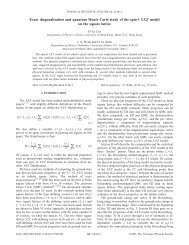
338 H.Y. Shik et al. / Nuclear <strong>Physics</strong> B 666 [FS] (2003) 337–360<br />
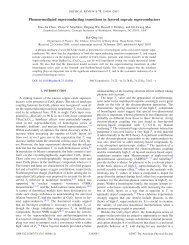
Fig. 1. The net <strong>spin</strong> layer <strong>of</strong> 2KL <strong>spin</strong>, where thick solid lines represent singlet dimers.<br />
studies [9–13]. There exist a few <strong>soluble</strong> <strong>quantum</strong> <strong>spin</strong> <strong>models</strong> for ladders and other<br />
systems in literature [14–21].<br />
Recently, we have shown [22] that there exists a class <strong>of</strong> exact <strong>soluble</strong> <strong>quantum</strong> <strong>spin</strong><br />
model for any <strong>spin</strong> S in one and two dimensions. We call it the net <strong>spin</strong> model. As shown<br />
in Fig. 1, each layer has K × L sites where <strong>spin</strong>s interact with their nearest-neighbors via<br />
coupling J 2 . Between layers, <strong>spin</strong> S with S =|S|=1/2, 1,...,sits on one layer connects<br />
to <strong>spin</strong> S ′ on the other layer not only perpendicularly by coupling J 1 , but also diagonally<br />
by J 3 and J 4 . L is the measure <strong>of</strong> the dimensionality varying from 1 (one dimension) to K<br />
(two dimensions). The net <strong>spin</strong> model is described by the Hamiltonian:<br />
∑K,L<br />
H = 2J 1<br />
k,l=1<br />
S k,l · S ′ k,l<br />
K−1,L−1<br />
∑<br />
+ 2J 2<br />
k,l=1<br />
K−1,L−1<br />
∑<br />
+ 2J 3<br />
k,l=1<br />
K−1,L−1<br />
∑<br />
+ 2J 4<br />
k,l=1<br />
S k,l · (S k+1,l + S k,l+1 ) + S ′ k,l · (S′ k+1,l + S′ k,l+1 )<br />
S ′ k,l · (S k+1,l + S k,l+1 )<br />
S k,l · (S ′ k+1,l + S′ k,l+1 ).<br />
We have shown that under the condition 2J 2 = J 3 + J 4 , the completely dimerized state<br />
ψ D , where <strong>spin</strong>s on the lower layer form dimers with <strong>spin</strong>s on the upper layer, is an<br />
eigenstate <strong>of</strong> Eq. (1). When J 1 is sufficiently large, ψ D is also the ground state. In addition,<br />
we also found that wave functions such as the single magnon state ψ m , the double magnon<br />
state ψ m,m ′, and four-<strong>spin</strong> plaquette singlet state ψ ✷ are also eigenstates <strong>of</strong> the model.<br />
These particular wave functions are:<br />
(1)<br />
ψ D =[1, 1 ′ ][2, 2 ′ ]···[KL,K ′ L ′ ],<br />
ψ m =[1, 1 ′ ]···(i, i ′ ) ···[KL,K ′ L ′ ],<br />
ψ m,m ′ =[1, 1 ′ ]···(i, i ′ )[j,j ′ ](k, k ′ ) ···[KL,K ′ L ′ ],<br />
ψ ✷ =[1, 1 ′ ]···{✷}···[KL,KL ′ ],<br />
(2)<br />
(3)<br />
(4)<br />
(5)
H.Y. Shik et al. / Nuclear <strong>Physics</strong> B 666 [FS] (2003) 337–360 339<br />
where [i, i ′ ] denotes a normalized <strong>spin</strong> singlet with |S i + S ′ i<br />
|=0, e.g., for the <strong>spin</strong>-1/2<br />
case,<br />
[i, i ′ ]= 1 √<br />
2<br />
( |↑i ↓ i ′〉−|↓ i ↑ i ′〉 ) ,<br />
(6)<br />
(i, i ′ ) denotes a normalized non-singlet such as triplet or pentad with |S i + S ′ i<br />
|=m ≠ 0,<br />
e.g., for the <strong>spin</strong>-1/2 case and m = 1<br />
(i, i ′ ) =− 1 √<br />
2<br />
( |↑i ↑ i ′〉−|↓ i ↓ i ′〉 ) ,<br />
i<br />
√<br />
2<br />
(<br />
|↑i ↑ i ′〉+|↓ i ↓ i ′〉 ) ,<br />
or<br />
or<br />
1<br />
√<br />
2<br />
(<br />
|↑i ↓ i ′〉+|↓ i ↑ i ′〉 ) ,<br />
(7)<br />
and {✷} denotes the four-<strong>spin</strong> plaquette singlet with |S i + S ′ i + S i+1 + S ′ i+1<br />
|=0, e.g., for<br />
the <strong>spin</strong>-1/2 case,<br />
{✷}= 1 (∣ 〉<br />
∣∣∣ ↓↓<br />
√ +<br />
(8)<br />
12 ↑↑ ∣ ↓↑ 〉<br />
+<br />
↑↓ ∣ ↑↓ 〉<br />
+<br />
↓↑ ∣ ↑↑ 〉<br />
− 2<br />
↓↓ ∣ ↓↑ 〉<br />
− 2<br />
↓↑ ∣ ↑↓ 〉)<br />
,<br />
↑↓<br />
with ↑ and ↓ representing the z-component <strong>of</strong> single <strong>spin</strong> being equal to 1/2 and−1/2,<br />
respectively.<br />
Thus a subset <strong>of</strong> the Hilbert <strong>of</strong> the net <strong>spin</strong> model is exactly known. We investigated the<br />
ground state and the excitation gap in detail for a wide range <strong>of</strong> parameters and varying<br />
dimensionality L from L = 1 (one dimension we call it net <strong>spin</strong> ladder) to L = K (two<br />
dimensions we call it net <strong>spin</strong> layer). Our main findings were: (i) let coupling J 1 define<br />
the energy scale <strong>of</strong> the model, when other couplings increase, the ground state changes<br />
from the completely dimerized state ψ D to the ground state <strong>of</strong> the <strong>spin</strong>-σ (σ = 2S) model<br />
defined on the single layer; (ii) the model exhibits rich excitation phases with distinct<br />
behaviors in one and two dimensions; (iii) dimensional crossover for <strong>spin</strong> S = 1/2 was<br />
identified. Finally, we note that at a particular point in the parameter space: S = 1/2,<br />
L = 1, J 2 = 1 2 J 1, J 3 = J 1 ,andJ 4 = 0 the net <strong>spin</strong> model goes back to the MG model [4].<br />
Therefore, the net <strong>spin</strong> model is a generalization <strong>of</strong> the MG model for any <strong>spin</strong> S in one<br />
and two dimensions.<br />
In this paper, we search for other exactly <strong>soluble</strong> <strong>spin</strong> <strong>models</strong> in two and three<br />
dimensions. To this purpose, we apply an operator approach, the bond operator method.<br />
In spirit, this approach is similar to techniques used for constructing integrable fermionic<br />
<strong>models</strong> [23]. First, in Section 2 we review the bond operator for the <strong>spin</strong>-1/2 case and<br />
introduce the bond operator for the <strong>spin</strong>-1 case, with briefly discussion <strong>of</strong> the bond operator<br />
for the general <strong>spin</strong>-S case. Then in Section 3 we use the bond operator to rewrite the<br />
Hamiltonian Eq. (1) in such a way that one can obtain the condition(s) for the completely<br />
dimerized state being an eigenstate <strong>of</strong> the Hamiltonian immediately. Afterwards, we<br />
present several two-dimensional (single layer) and three-dimensional <strong>soluble</strong> <strong>quantum</strong> <strong>spin</strong><br />
<strong>models</strong> in Sections 4 and 5, followed by a short summary in Section 6.
340 H.Y. Shik et al. / Nuclear <strong>Physics</strong> B 666 [FS] (2003) 337–360<br />
2. Bond operator<br />
2.1. Spin-1/2 bond operator<br />
In this section, the so called “bond operator” representation is discussed. For a dimer<br />
consisting <strong>of</strong> two <strong>spin</strong>s S and S ′ , instead <strong>of</strong> using the <strong>spin</strong> operator representation for S α<br />
and S α ′ ,whereα = x,y,z, an alternative representation, known as the bond operator could<br />
also be used. Such representation was first introduced by Sachdev and Bhatt in 1990 [1],<br />
in which the original two <strong>spin</strong>-1/2 operators, S and S ′ , are represented by four bosonic<br />
operators s † ,t x † ,t y † and t z † , which create the singlet state |s〉 and triplet states |t x 〉, |t y 〉,and<br />
|t z 〉 out <strong>of</strong> the vacuum state |vac〉, respectively,<br />
|s〉≡s † |vac〉= 1 ( )<br />
√ |↑↓〉 − |↓↑〉 , (9)<br />
2<br />
|t x 〉≡t † −1 ( )<br />
x |vac〉= √ |↑↑〉 − |↓↓〉 , (10)<br />
2<br />
|t y 〉≡t y † |vac〉= i ( )<br />
√ |↑↑〉 + |↓↓〉 , (11)<br />
2<br />
(12)<br />
|t z 〉≡t † z |vac〉= 1 √<br />
2<br />
(<br />
|↑↓ + |↓↑〉<br />
)<br />
,<br />
and conversely<br />
S α = 1 s<br />
2( † t α + t α † s − iɛ αβγ t † β t )<br />
γ ,<br />
(13)<br />
S ′ α = 1 2(<br />
−s † t α − t † α s − iɛ αβγ t † β t γ<br />
)<br />
,<br />
where α, β, andγ take the values <strong>of</strong> x,y,andz. The Levi-Civita symbol ɛ is the totally<br />
antisymmetric tensor, and all repeated indices are summed over. For physical state there is<br />
either a singlet or triplet, so the following constraint should be imposed,<br />
s † s + t † α t α = 1.<br />
(14)<br />
2.2. Spin-1 bond operator<br />
Similar to the <strong>spin</strong>-1/2 case, we can construct the <strong>spin</strong>-1 bond operators. We leave their<br />
constructions to Appendix A. The original two <strong>spin</strong>-1 operators, S and S ′ , are represented<br />
by nine bosonic operators s † , t † 1 , t† 0 , t† −1 , p† 2 , p† 1 , p† 0 , p† −1 and p† −2<br />
which create the<br />
singlet state |s〉, triplet states |t α 〉, and pentad states |p β 〉 out <strong>of</strong> the vacuum state |vac〉,<br />
respectively.<br />
The singlet |s〉 is defined as<br />
|s〉≡s † |vac〉= 1 √<br />
3<br />
(<br />
|↑↓〉 − |00〉 + |↓↑〉<br />
)<br />
.<br />
(15)
H.Y. Shik et al. / Nuclear <strong>Physics</strong> B 666 [FS] (2003) 337–360 341<br />
The triplets |t α 〉 with α =±1and0beingthez-component <strong>of</strong> the total <strong>spin</strong> are defined<br />
as<br />
|t 1 〉≡t † 1 |vac〉= 1<br />
(16)<br />
√<br />
2<br />
(<br />
|0↑〉 − |↑0〉<br />
)<br />
,<br />
(17)<br />
|t 0 〉≡t † 0 |vac〉= 1 √<br />
2<br />
(<br />
|↓↑〉 − |↑↓〉<br />
)<br />
,<br />
(18)<br />
|t −1 〉≡t † −1 |vac〉= 1 √<br />
2<br />
(<br />
|↓0〉−|0↓〉<br />
)<br />
.<br />
The fivefold multiplets pentad |p β 〉 with β =±2, ±1, and 0 are defined as<br />
|p 2 〉≡p † 2 |vac〉 = |↑↑〉, (19)<br />
(20)<br />
|p 1 〉≡p † 1 |vac〉= 1 √<br />
2<br />
( |0↑〉 + |↑0〉<br />
) ,<br />
(21)<br />
|p 0 〉≡p † 0 |vac〉= 1 √<br />
6<br />
(<br />
|↑↓〉 + 2|00〉 + |↓↑〉<br />
)<br />
,<br />
(22)<br />
Conversely,<br />
|p −1 〉≡p † −1 |vac〉= 1 √<br />
2<br />
(<br />
|0↓〉 + |↓0〉<br />
)<br />
,<br />
(23)<br />
|p −2 〉≡p † −2 |vac〉=|↓↓〉.<br />
S z<br />
= p † 2 p 2 + 1 2 p† 1 p 1 − 1 2 p† −1 p −1 − p † −2 p −2 + 1 2 t† 1 t 1 − 1 2 t† −1 t −1<br />
− 1 2<br />
(<br />
p<br />
†<br />
1 t 1 + t † 1 p ) 1 (<br />
1 − √3 p<br />
†<br />
0 t 0 + t † 0 p 0<br />
) 1( − p<br />
†<br />
−1<br />
2<br />
t −1 + t † −1 p )<br />
−1<br />
−<br />
√<br />
2 (<br />
t<br />
†<br />
0<br />
3<br />
s + ) s† t 0 ,<br />
S ′ z = p † 2 p 2 + 1 2 p† 1 p 1 − 1 2 p† −1 p −1 − p † −2 p −2 + 1 2 t† 1 t 1 − 1 2 t† −1 t −1<br />
+ 1 2<br />
+<br />
(<br />
p<br />
†<br />
1 t 1 + t † 1 p ) 1 (<br />
1 + √3 p<br />
†<br />
0 t 0 + t † 0 p 0<br />
√<br />
2 (<br />
t<br />
†<br />
3<br />
0 s + s† t 0<br />
)<br />
,<br />
S + = p † 2 p 1 + p † −1 p −2 +<br />
) 1( + p<br />
†<br />
2<br />
−1 t −1 + t † −1 p )<br />
−1<br />
√<br />
3 (<br />
p<br />
†<br />
1<br />
2<br />
p 0 + p † 0 p ) 1 (<br />
−1 + √2 t<br />
†<br />
1 t 0 + t † 0 t )<br />
−1<br />
+ p † 2 t 1 − t † −1 p −2 + √ 1 (<br />
p<br />
†<br />
1 t 0 − t † 0 p ) 1 (<br />
−1 + √6 p<br />
†<br />
0 t −1 − t † 1 p )<br />
0<br />
2<br />
+ 2 √<br />
3<br />
( t<br />
†<br />
1 s − s† t −1<br />
) ,
342 H.Y. Shik et al. / Nuclear <strong>Physics</strong> B 666 [FS] (2003) 337–360<br />
√<br />
S ′+ = p † 2 p 1 + p † 3<br />
−1 p (<br />
−2 + p<br />
†<br />
2<br />
1 p 0 + p † 0 p ) 1 (<br />
−1 + √2 t<br />
†<br />
1 t 0 + t † 0 t )<br />
−1<br />
− p † 2 t 1 + t † −1 p −2 − √ 1 ( p<br />
†<br />
1 t 0 − t † 0 p ) 1 (<br />
−1 − √6 p<br />
†<br />
0 t −1 − t † 1 p )<br />
0<br />
2<br />
− 2 √<br />
3<br />
(<br />
t<br />
†<br />
1 s − s† t −1<br />
)<br />
.<br />
(24)<br />
Since physical states are either singlet, triplet, or pentad, the following constraint is<br />
imposed<br />
s † s + t α † t α + p † β p β = 1,<br />
(25)<br />
where α =±1, 0andβ =±2, ±1, 0.<br />
For general <strong>spin</strong>-S, its bond operator representation could also be obtained, in principle.<br />
However, when <strong>spin</strong> S increases, the number <strong>of</strong> bosonic operators required to represent the<br />
<strong>spin</strong> operators S and S ′ is (2S + 1) 2 , which increases exponentially. More discussions are<br />
given in Appendix B.<br />
3. Bond operator representation <strong>of</strong> the net <strong>spin</strong> model<br />
By using the bond operator representation, it is easy to see that the condition 2J 2 =<br />
J 3 + J 4 makes the completely dimerized state ψ D be the eigenstate <strong>of</strong> the net <strong>spin</strong> model.<br />
As an illustration, we study the <strong>spin</strong>-1/2 case in two dimensions. Substituting bosonic<br />
operators for the <strong>spin</strong> operators, as defined in Eq. (13), we rewrite the net <strong>spin</strong> Hamiltonian<br />
Eq. (1) as<br />
H = 2J 1 h 1 + 2(2J 2 − J 3 − J 4 )h 2 + 2(J 3 − J 4 )h 3 + 2(J 2 + J 3 + J 4 )h 4 ,<br />
where<br />
K,L<br />
∑<br />
(<br />
h 1 = − 3 4 s† k,l s k,l + 1 )<br />
4 t† αk,l t αk,l ,<br />
h 2 =<br />
k,l=1<br />
K−1,L−1<br />
∑<br />
k,l=1<br />
1<br />
4<br />
(<br />
s<br />
†<br />
k,l t αk,ls † k+1,l t αk+1,l + s † k,l t αk,lt † αk+1,l s k+1,l<br />
+ t † αk,l s k,ls † k+1,l t αk+1,l + t † αk,l s k,lt † αk+1,l s k+1,l<br />
(26)<br />
K−1,L−1<br />
∑<br />
h 3 =<br />
k,l=1<br />
i<br />
4 ɛ αβγ<br />
+ s † k,l t αk,ls † k,l+1 t αk,l+1 + s † k,l t αk,lt † αk,l+1 s k,l+1<br />
+ t † αk,l s k,ls † k,l+1 t αk,l+1 + t † αk,l s k,lt † αk,l+1 s k,l+1<br />
(<br />
s<br />
†<br />
k,l t αk,lt † βk+1,l t γk+1,l + t † αk,l s k,lt † βk+1,l t γk+1,l<br />
− t † βk,l t γk,ls † k+1,l t αk+1,l − t † βk,l t γk,lt † αk+1,l s k+1,l<br />
(27)<br />
) ,<br />
(28)<br />
+ s † k,l t αk,lt † βk,l+1 t γk,l+1 + t † αk,l s k,lt † βk,l+1 t γk,l+1<br />
− t † βk,l t γk,ls † k,l+1 t αk,l+1 − t † βk,l t γk,lt † αk,l+1 s k,l+1)<br />
,
H.Y. Shik et al. / Nuclear <strong>Physics</strong> B 666 [FS] (2003) 337–360 343<br />
h 4 =<br />
K−1,L−1<br />
∑<br />
k,l=1,α≠β<br />
1<br />
4 t† αk,l t (<br />
βk,l tαk+1,l t † βk+1,l − t† αk+1,l t βk+1,l<br />
+ t αk,l+1 t † βk,l+1 − t† αk,l+1 t βk,l+1)<br />
.<br />
(29)<br />
In Eq. (26), h 1 is diagonal in boson number operators. All the remaining four-operator<br />
terms (h 2 ,h 3 and h 4 ) give zero when they act on the completely dimerized state ψ D except<br />
the terms t † αk,l s k,lt † αk+1,l s k+1,l and t † αk,l s k,lt † αk,l+1 s k,l+1 in h 2 .Sincet † αi s it † αj s j will destroy<br />
a singlet and create a triplet on both sites i and j, a new state is created, i.e.,<br />
t † αi s it † αj s j ψ D =[1, 1 ′ ]···(i, i ′ )(j, j ′ ) ···[KL,K ′ L ′ ].<br />
(30)<br />
So to make the completely dimerized state ψ D be an eigenstate, the coefficient <strong>of</strong> h 2<br />
must be zero, which leads to the condition 2J 2 = J 3 + J 4 .<br />
If J 2 = J 3 = J 4 , the Hamiltonian becomes<br />
∑K,L<br />
H = 2J 1<br />
k,l=1<br />
K−1,L−1<br />
∑<br />
+ 2J 2<br />
(<br />
− 3 4 s† k,l s k,l + 1 )<br />
4 t† αk,l t αk,l<br />
k,l=1,α≠β<br />
t † αk,l t βk,l(<br />
tαk+1,l t † βk+1,l + t αk,l+1t † βk,l+1<br />
− t † αk+1,l t βk+1,l − t † αk,l+1 t βk,l+1)<br />
.<br />
(31)<br />
By inspecting the above simplified Hamiltonian, we immediately see that the eigenvalue<br />
<strong>of</strong> the completely dimerized state E D is −2J 1 × 3/4 × N where N = KL is the total<br />
number <strong>of</strong> singlets on the double layer. Moreover, in the large J 1 limit, the completely<br />
dimerized state is the ground state and the first excited state should be a single magnon<br />
created by breaking a dimer at any site, with eigenvalue E D + 2J 1 . Thus, without solving<br />
the Hamiltonian explicitly, useful information are already revealed by the bond operator<br />
representation <strong>of</strong> the model.<br />
For general <strong>spin</strong>-S case, similar approach will lead to the same conclusions. In order not<br />
to bore the readers, the derivations is not shown here. Instead, we present the derivations<br />
for the <strong>spin</strong>-1 case for a three-dimensional model in Section 5 and leave the derivations for<br />
general <strong>spin</strong>-S case to Appendix B.<br />
4. Two-dimensional exactly <strong>soluble</strong> model<br />
In this section, we construct other exactly <strong>soluble</strong> <strong>models</strong> in two dimensions by applying<br />
the bond operator method. Obviously, there could be a lot. A simple case would be a natural<br />
continuation <strong>of</strong> the net <strong>spin</strong> model where one connects a set <strong>of</strong> ladders by inter-ladder<br />
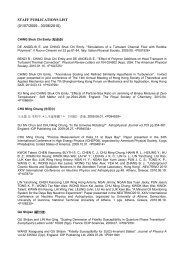
couplings J 5 ,J 6 ,J 7 ,andJ 8 as shown in Fig. 2.
344 H.Y. Shik et al. / Nuclear <strong>Physics</strong> B 666 [FS] (2003) 337–360<br />
Fig. 2. The nested-ladder model.<br />
In Fig. 2, m and m ′ label the lower and upper hand <strong>of</strong> ladder, respectively, and there are<br />
total <strong>of</strong> M ladders. The Hamiltonian <strong>of</strong> the model in Fig. 2 is<br />
K,M<br />
∑<br />
H = 2J 1<br />
k,m=1<br />
K−1,M<br />
∑<br />
+ 2J 3<br />
S k,m · S ′ k,m + 2J 2<br />
k,m=1<br />
K,M−1<br />
∑<br />
+ 2J 5<br />
k,m=1<br />
K,M−1<br />
∑<br />
+ 2J 7<br />
k,m=1<br />
K−1,M<br />
∑<br />
k,m=1<br />
S k+1,m · S ′ k,m + 2J 4<br />
(S k,m · S k+1,m + S ′ k,m · S′ k+1,m )<br />
K−1,M<br />
∑<br />
k,m=1<br />
K,M−1<br />
S ′ k,m · S ∑<br />
k,m+1 + 2J 6<br />
k,m=1<br />
K,M−1<br />
∑<br />
S k,m · S k,m+1 + 2J 8<br />
k,m=1<br />
S k,m · S ′ k+1,m<br />
S ′ k,m · S′ k,m+1<br />
S k,m · S ′ k,m+1 .<br />
To be definitive, we refer the bond operator for <strong>spin</strong> S k,m and S ′ k,m<br />
. Substituting Eq. (13)<br />
into the Hamiltonian Eq. (32), we get<br />
(32)<br />
H = 2J 1 h 1 + 2(2J 2 − J 3 − J 4 )h 2a + 2(J 6 + J 7 − J 5 − J 8 )h 2b + 2(J 3 − J 4 )h 3a<br />
+ 2(J 8 − J 5 )h 3b + 2(2J 2 + J 3 + J 4 )h 4a + 2(J 5 + J 6 + J 7 + J 8 )h 4b , (33)<br />
where<br />
h 1 =<br />
K,M<br />
∑<br />
k,m=1<br />
(<br />
− 3 4 s† k,m s k,m + 1 )<br />
4 t† αk,m t αk,m ,<br />
(34)
H.Y. Shik et al. / Nuclear <strong>Physics</strong> B 666 [FS] (2003) 337–360 345<br />
K−1,M<br />
∑ 1( h 2a = s<br />
†<br />
k,m<br />
4<br />
t αk,ms † k+1,m t αk+1,m + s † k,m t αk,mt † αk+1,m s k+1,m<br />
k,m=1<br />
+ t † αk,m s k,ms † k+1,m t αk+1,m + t † αk,m s k,mt † αk+1,m s k+1,m<br />
K,M−1<br />
∑ 1 (<br />
h 2b = s<br />
†<br />
k,m<br />
4<br />
t αk,ms † k,m+1 t αk,m+1 + s † k,m t αk,mt † αk,m+1 s k,m+1<br />
k,m=1<br />
(35)<br />
)<br />
,<br />
(36)<br />
+ t † αk,m s k,ms † k,m+1 t αk,m+1 + t † αk,m s k,mt † αk,m+1 s )<br />
k,m+1 ,<br />
(37)<br />
K−1,M<br />
∑ i<br />
h 3a =<br />
4 ɛ (<br />
αβγ s<br />
†<br />
k,m t αk,mt † βk+1,m t γk+1,m + t † αk,m s k,mt † βk+1,m t γk+1,m<br />
k,m=1<br />
− t † βk,m t γk,ms † k+1,m t αk+1,m − t † βk,m t γk,mt † αk+1,m s )<br />
k+1,m ,<br />
(38)<br />
K,M−1<br />
∑ i<br />
h 3b =<br />
4 ɛ (<br />
αβγ s<br />
†<br />
k,m t αk,mt † βk,m+1 t γk,m+1 + t † αk,m s k,mt † βk,m+1 t γk,m+1<br />
k,m=1<br />
h 4a =<br />
h 4b =<br />
K−1,M<br />
∑<br />
k,m=1,α≠β<br />
K,M−1<br />
∑<br />
k,m=1,α≠β<br />
− t † βk,m t γk,ms † k,m+1 t αk,m+1 − t † βk,m t γk,mt † αk,m+1 s )<br />
k,m+1 ,<br />
) , (39)<br />
(40)<br />
1<br />
4 t† αk,m t (<br />
βk,m tαk+1,m t † βk+1,m − t† αk+1,m t βk+1,m<br />
1<br />
4 t† αk,m t (<br />
βk,m tαk,m+1 t † βk,m+1 − t† αk,m+1 t )<br />
βk,m+1 .<br />
Then, based on the arguments we have in previous sections, the conditions for the<br />
completely dimerized state to be an eigenstate are<br />
2J 2 = J 3 + J 4 , J 6 + J 7 = J 5 + J 8 .<br />
(41)<br />
Again, as in the previous section, same conditions hold for cases with <strong>spin</strong> S other<br />
than 1/2. Conditions Eq. (41) could have various forms. For example, we can let J 6 = J 7<br />
due to symmetry and let J 8 = 0togetJ 5 = 2J 6 ,orletJ 5 = J 6 = J 7 = J 8 and study their<br />
energy specturms. In fact, then the model could be maped into coupled <strong>spin</strong> chains with<br />
spatial anisotropy. Quantum phase transitions are expected. We also remark that one can<br />
obtain <strong>soluble</strong> bilayer net <strong>spin</strong> model with inter-bilayer couplings under similar conditions.<br />
5. Three-dimensional exactly <strong>soluble</strong> model<br />
In this section, the bond operator method is used to determine the condition(s) required<br />
for the completely dimerized state to be an eigenstate <strong>of</strong> a three-dimensional model H 3D ,<br />
defined by the Hamiltonian,<br />
K,L,M<br />
∑<br />
K,L,M−1<br />
H 3D = 2J 1 S k,l,m · S ′ k,l,m + 2 ∑<br />
J˜<br />
1 S ′ k,l,m · S k,l,m+1<br />
k,l,m=1<br />
k,l,m=1
346 H.Y. Shik et al. / Nuclear <strong>Physics</strong> B 666 [FS] (2003) 337–360<br />
K−1,L−1,M<br />
∑<br />
+ 2J 2<br />
k,l,m=1<br />
S k,l,m · (S k+1,l,m + S k,l+1,m )<br />
+ S ′ k,l,m · (S′ k+1,l,m + S′ k,l+1,m )<br />
K−1,L−1,M<br />
∑<br />
+ 2J 3 S ′ k,l,m · (S k+1,l,m + S k,l+1,m )<br />
+ 2 ˜<br />
+ 2J ‖ 3<br />
k,l,m=1<br />
K−1,L−1,M−1<br />
∑<br />
J 3<br />
k,l,m=1<br />
K−1,L−1,M<br />
∑<br />
k,l,m=1<br />
K−1,L−1,M<br />
∑<br />
+ 2J 4<br />
+ 2 ˜<br />
+ 2J ‖ 4<br />
k,l,m=1<br />
K−1,L−1,M−1<br />
∑<br />
J 4<br />
k,l,m=1<br />
K−1,L−1,M<br />
∑<br />
k,l,m=1<br />
K−1,L−1,M<br />
∑<br />
+ 2J 5<br />
+ 2 ˜<br />
k,l,m=1<br />
K−1,L−1,M−1<br />
∑<br />
J 5<br />
k,l,m=1<br />
K,L,M−1<br />
∑<br />
+ 2J 6<br />
+ 2J ‖ 6<br />
k,l,m=1<br />
K−2,L−2,M<br />
∑<br />
k,l,m=1<br />
S k,l,m+1 · (S ′ k+1,l,m + S′ k,l+1,m )<br />
S k+1,l,m · S k,l+1,m + S ′ k+1,l,m · S′ k,l+1,m<br />
S k,l,m · (S ′ k+1,l,m + S′ k,l+1,m )<br />
S ′ k,l,m · (S k+1,l,m+1 + S k,l+1,m+1 )<br />
S k,l,m · S k+1,l+1,m + S ′ k,l,m · S′ k+1,l+1,m<br />
S k,l,m · S ′ k+1,l+1,m + S k+1,l,m · S ′ k,l+1,m<br />
+ S k,l+1,m · S ′ k+1,l,m + S k+1,l+1,m · S ′ k,l,m<br />
S ′ k,l,m · S k+1,l+1,m+1 + S ′ k+1,l,m · S k,l+1,m+1<br />
+ S ′ k,l+1,m · S k+1,l,m+1 + S ′ k+1,l+1,m · S k,l,m+1<br />
S k,l,m · S k,l,m+1 + S ′ k,l,m · S′ k,l,m+1<br />
S k,l,m · (S k+2,l,m + S k,l+2,m )<br />
+ S ′ k,l,m · (S′ k+2,l,m + S′ k,l+2,m )<br />
K−2,L−2,M<br />
∑<br />
+ 2J 7 S k,l,m · (S ′ k+2,l,m + S′ k,l+2,m )<br />
k,l,m=1<br />
+ S ′ k,l,m · (S k+2,l,m + S k,l+2,m )
H.Y. Shik et al. / Nuclear <strong>Physics</strong> B 666 [FS] (2003) 337–360 347<br />
+ 2 ˜<br />
+ 2J ‖ 7<br />
K−2,L−2,M−1<br />
∑<br />
J 7<br />
k,l,m=1<br />
K−2,L−2,M<br />
∑<br />
k,l,m=1<br />
S ′ k,l,m · (S k+2,l,m+1 + S k,l+2,m+1 )<br />
+ S k,l,m+1 · (S ′ k+2,l,m + S′ k,l+2,m )<br />
S k,l,m · (S k+2,l+1,m + S k+1,l+2,m )<br />
+ S ′ k,l,m · (S′ k+2,l+1,m + S′ k+1,l+2,m )<br />
+ S k,l+2,m · (S k+1,l,m + S k+2,l+1,m )<br />
+ S ′ k,l+2,m · (S′ k+1,l,m + S′ k+2,l+1,m )<br />
K−1,L−1,M−1<br />
∑<br />
+ 2J 8 S k,l,m · (S k+1,l,m+1 + S k,l+1,m+1 )<br />
k,l,m=1<br />
+ S ′ k,l,m · (S′ k+1,l,m+1 + S′ k,l+1,m+1 )<br />
+ S k,l,m+1 · (S k+1,l,m + S k,l+1,m )<br />
+ S ′ k,l,m+1 · (S′ k+1,l,m + S′ k,l+1,m )<br />
K−1,L−1,M−1<br />
∑<br />
+ 2J 9 S k,l,m · S k+1,l+1,m+1 + S k+1,l,m · S k,l+1,m+1<br />
k,l,m=1<br />
+ S k+1,l+1,m · S k,l,m+1 + S k,l+1,m · S k+1,l,m+1<br />
+ S ′ k,l,m · S′ k+1,l+1,m+1 + S′ k+1,l,m · S′ k,l+1,m+1<br />
K−2,L−1,M−1<br />
∑<br />
+ 2J 10<br />
+ 2 ˜<br />
k,l,m=1<br />
K−2,L−1,M−1<br />
∑<br />
J 10<br />
k,l,m=1<br />
K−2,L−2,M<br />
∑<br />
+ 2J 11<br />
+ 2J ‖ 11<br />
k,l,m=1<br />
K−2,L−2,M<br />
∑<br />
k,l,m=1<br />
+ S ′ k+1,l+1,m · S′ k,l,m+1 + S′ k,l+1,m · S′ k+1,l,m+1<br />
S k,l,m · S ′ k+2,l+1,m + S k+2,l,m · S ′ k,l+1,m<br />
+ S k+2,l+1,m · S ′ k,l,m + S k,l+1,m · S ′ k+2,l,m<br />
S ′ k,l,m · S k+2,l+1,m+1 + S ′ k+2,l,m · S k,l+1,m+1<br />
+ S ′ k+2,l+1,m · S k,l,m+1 + S ′ k,l+1,m · S k+2,l,m+1<br />
S k,l,m · (S k+2,l,m+1 + S k,l+2,m+1 )<br />
+ S ′ k,l,m · (S′ k+2,l,m+1 + S′ k,l+2,m+1 )<br />
+ S k,l,m+1 · (S k+2,l,m + S k,l+2,m )<br />
+ S ′ k,l,m+1 · (S′ k+2,l,m + S′ k,l+2,m )<br />
S k,l,m · S k+2,l+2,m + S ′ k,l,m · S′ k+2,l+2,m<br />
+ S k,l+2,m · S k+2,l,m + S ′ k,l+2,m · S′ k+2,l,m .<br />
(42)
348 H.Y. Shik et al. / Nuclear <strong>Physics</strong> B 666 [FS] (2003) 337–360<br />
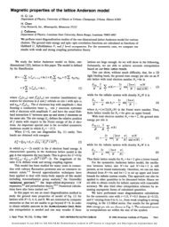
Fig. 3. The labelling scheme <strong>of</strong> the three-dimensional model.<br />
We draw the three-dimensional model considered in Fig. 3. Let the lattice separation<br />
be one and we include all couplings with separation no larger than 2 √ 2. There are total<br />
<strong>of</strong> twenty-two couplings. Since the couplings J 10 and J˜<br />
10 cannot be grouped in the bond<br />
representation, we have to discard them. The Hamiltonian looks rather complicated but<br />
it is basically built up by the bilayer net <strong>spin</strong> model. Couplings between the bilayers are<br />
specified with tilde (˜), while those lie on the xy-plane are labelled with parallel sign (‖).<br />
Specifically:<br />
Separation<br />
Coupling(s) included<br />
1 J 1 , J˜<br />
1 ,J<br />
√ 2<br />
2<br />
J3 , J˜<br />
3 ,J ‖ 3 ,J 4, J˜<br />
√ 4 ,J ‖ 4<br />
3<br />
J5 , ˜<br />
2 J 6 ,J ‖ 6<br />
√<br />
5<br />
J7 , J˜<br />
7 ,J ‖ 7 ,J 8<br />
√<br />
6<br />
J9 ,(J 10 , J˜<br />
10 )<br />
2 √ 2 J 11 ,J ‖ 11<br />
J 5<br />
The bond operator representations <strong>of</strong> the Hamiltonian Eq. (42) for the <strong>spin</strong>-1/2 case<br />
is too tedious to present here, readers who are interested could ask us for manuscript.<br />
Basically we combine terms according to combinations <strong>of</strong> creation and annihilation boson<br />
operators. Straightforward manipulations lead to the following conditions which make the<br />
completely dimerized state be an eigenstate <strong>of</strong> the Hamiltonian Eq. (42):<br />
2J 2 = J 3 + J 4 , 2J 5 = J ‖ 3 + J ‖ 4 , J‖ 6 = J 7, 2J 6 = J˜<br />
1 ,<br />
2J 8 = ˜ J 3 = ˜ J 4 ,<br />
2J 9 = ˜ J 5 ,<br />
2J 11 = ˜ J 7 , J ‖ 7 ,J‖ 11 = 0.<br />
(43)
H.Y. Shik et al. / Nuclear <strong>Physics</strong> B 666 [FS] (2003) 337–360 349<br />
As a demonstration, we present derivations for the <strong>spin</strong>-1 case here. Obviously,<br />
expression <strong>of</strong> the Hamiltonian in terms <strong>of</strong> bond operators is even more complicated.<br />
However, since the main concern is about how H 3D Eq. (42) acts on the completely<br />
dimerized state ψ D , only terms consisting <strong>of</strong> singlet operator s need to be considered.<br />
Hence, one can simplify the expression <strong>of</strong> the bond operator representation by keeping the<br />
terms with singlet operator s only,<br />
√<br />
2<br />
S z =−S ′ z (<br />
→− t<br />
†<br />
3<br />
(44)<br />
and<br />
0 s + ) s† t 0 ,<br />
√<br />
2<br />
S + =−S ′+ (<br />
→ t<br />
†<br />
1<br />
(45)<br />
3<br />
s − ) s† t −1 ,<br />
(46)<br />
S i =−S ′ i .<br />
S i · S j ψ D = S ′ i · S′ j ψ D =−S i · S ′ j ψ D =−S ′ i · S j ψ D .<br />
Thus, the bond operator representation for the four <strong>spin</strong> interactions, (S i · S j , S ′ i · S′ j , S i ·<br />
S ′ j , S′ i · S j ) are now the same upto a sign. So we only need to consider one <strong>of</strong> them, say,<br />
S i · S j ,<br />
(47)<br />
S i · S j = Si z Sz j + 2( 1 S<br />
+<br />
i<br />
Sj − + ) S− i S+ j ,<br />
(48)<br />
when for i ≠ j<br />
S z i Sz j = 2 3<br />
( t<br />
†<br />
(49)<br />
0i t† 0j s is j + t † 0i s† j s it 0j + s † i t† 0j t 0is j + s † i s† j t )<br />
0it 0j ,<br />
S<br />
i + Sj − = 4 (<br />
−t<br />
†<br />
(50)<br />
3<br />
1i t† −1j s is j + t † 1i s† j s it 1j + s † i t† −1j t −1is j − s † i s† j t )<br />
−1it 1j .<br />
When i = j, some four-operator terms will reduce to two-operator terms, e.g., t † 1i t 0it † 1j t 0j →<br />
t † 1i t 1i(1 + t † 0i t 0i) → t † 1i t 1i. Thus, we have to keep terms with t operators but neglect terms<br />
with p operators, i.e.,<br />
S z i Sz i → 1 2 t† 1i t 1i + t † 0i t 0i + 1 2 t† −1i t −1i + 2 3 s† i s i,<br />
S + i<br />
S − i<br />
→ 2t † 1i t 1i + t † 0i t 0i + t † −1i t −1i + 4 3 s† i s i,<br />
S − i<br />
S + i<br />
→ t † 1i t 1i + t † 0i t 0i + 2t † −1i t −1i + 4 3 s† i s i,<br />
(51)<br />
(52)<br />
(53)<br />
To simplify the expression, let us denote O i;j as<br />
O i;j ≡ 2 3<br />
(<br />
t<br />
†<br />
0i t† 0j s is j + t † 0i s† j s it 0j + s † i t† 0j t 0is j + s † i s† j t 0it 0j<br />
− t † 1i t† −1j s is j + t † 1i s† j s it 1j + s † i t† −1j t −1is j − s † i s† j t −1it 1j<br />
− t † −1i t† 1j s is j + t † −1i s† j s it −1j + s † i t† 1j t 1is j − s † i s† j t 1it −1j<br />
)<br />
.<br />
(54)
350 H.Y. Shik et al. / Nuclear <strong>Physics</strong> B 666 [FS] (2003) 337–360<br />
Finally, the Hamiltonian <strong>of</strong> the three-dimensional model Eq. (42) becomes (only the<br />
terms with s-operator are included),<br />
K,L,M<br />
∑ (<br />
H 3D → 2J 1 −2s<br />
†<br />
k,l,m s k,l,m − t † 1k,l,m t 1k,l,m − t † 0k,l,m t 0k,l,m − t † −1k,l,m t )<br />
−1k,l,m<br />
k,l,m=1<br />
K−1,L−1,M<br />
∑<br />
+ 2(2J 2 − J 3 − J 4 ) (O k,l,m;k+1,l,m + O k,l,m;k,l+1,m )<br />
K,L,M−1<br />
∑<br />
+ 2(2J 6 − J˜<br />
1 )<br />
+ 4 ( J ‖ 6 − J 7<br />
k,l,m=1<br />
) K−2,L−2,M ∑<br />
k,l,m=1<br />
k,l,m=1<br />
O k,l,m;k,l,m+1<br />
(O k,l,m;k+2,l,m + O k,l,m;k,l+2,m )<br />
K−1,L,M−1<br />
∑<br />
+ 2(2J 8 − J˜<br />
3 ) (O k,l,m+1;k+1,l,m + O k,l,m+1;k,l+1,m )<br />
k,l,m=1<br />
K−1,L,M−1<br />
∑<br />
+ 2(2J 8 − J˜<br />
4 ) (O k,l,m;k+1,l,m+1 + O k,l,m;k,l+1,m+1 )<br />
k,l,m=1<br />
K−2,L−2,M−1<br />
∑<br />
+ 2(2J 11 − J˜<br />
7 )<br />
(O k,l,m;k+2,l,m+1 + O k,l,m;k,l+2,m+1<br />
+ 4J ‖ 7<br />
K−2,L−2,M<br />
∑<br />
k,l,m=1<br />
+ 2 ( J ‖ 3 + J ‖ 4 − 2J 5<br />
+ 4J ‖ 11<br />
K−2,L−2,M<br />
∑<br />
k,l,m=1<br />
k,l,m=1<br />
+ O k,l,m+1;k+2,l,m + O k,l,m+1;k,l+2,m )<br />
(O k,l,m;k+2,l+1,m + O k+2,l,m;k,l+1,m<br />
+ O k,l,m;k+1,l+2,m + O k,l+2,m;k+1,l,m )<br />
) K,L,M ∑<br />
k,l,m=1<br />
(O k,l,m;k+1,l+1,m + O k+1,l,m;k,l+1,m )<br />
(O k,l,m;k+2,l+2,m + O k,l+2,m;k+2,l,m )<br />
K−1,L−1,M−1<br />
∑<br />
+ 2(2J 9 − J˜<br />
5 )<br />
(O k,l,m;k+1,l+1,m+1 + O k+1,l,m;k,l+1,m+1<br />
k,l,m=1<br />
+ O k,l+1,m;k+1,l,m+1 + O k+1,l+1,m;k,l,m+1 ).<br />
(55)<br />
With the same arguments used before, only the terms t † 0i t† 0j s is j ,t † 1i t† −1j s is j and<br />
t † −1i t† 1j s is j lead to non-dimer bases, which make the completely dimerized state not an
H.Y. Shik et al. / Nuclear <strong>Physics</strong> B 666 [FS] (2003) 337–360 351<br />
eigenstate. Hence, the coefficients <strong>of</strong> those terms are set to zero, which is Eq. (43) as for the<br />
<strong>spin</strong>-1/2 case. If all conditions are satisfied, the eigenenergy <strong>of</strong> the completely dimerized<br />
state is −2J 1 × 2 × N where N = KLM is the total number <strong>of</strong> dimers. In the limit <strong>of</strong> large<br />
J 1 , the excitation gap is 2J 1 and it is from singlet to triplet.<br />
Among these twenty-two couplings, J 1 is independent <strong>of</strong> the others, four <strong>of</strong> them<br />
(J ‖ 7 ,J 10, J˜<br />
10 ,J ‖ 11<br />
) should be zero if there is no further neighbor couplings considered,<br />
and the rests seventeen couplings are connected by the seven conditions as stated in<br />
Eq. (43). Various combinations <strong>of</strong> them will lead to a variety <strong>of</strong> <strong>quantum</strong> phase transitions.<br />
Note that those seven conditions on couplings are not all related for some <strong>of</strong> them are<br />
independent <strong>of</strong> the others. In the followings, we discuss a few <strong>soluble</strong> cases. The objective<br />
is to obtain <strong>soluble</strong> <strong>models</strong> with minimum number <strong>of</strong> couplings. For all the cases, the<br />
condition 2J 2 = J 3 + J 4 is always held.<br />
5.1. Double layer model I: 2J 5 = J ‖ 3 + J ‖ 4<br />
This condition leads to another double layer model for there is no connections between<br />
layers, as shown in Fig. 4. In this model, the effect <strong>of</strong> J ‖ 3 and J ‖ 4<br />
on the dimers are exactly<br />
cancelled out by J 5 which is very similar to the net <strong>spin</strong> model we proposed before where<br />
the effects <strong>of</strong> J 2 are cancelled out by J 3 and J 4 .<br />
5.2. Double layer model II: J ‖ 6 = J 7<br />
Another double layer model can be constructed by the condition J ‖ 6 = J 7 (Fig. 5). The<br />
<strong>quantum</strong> fluctuation due to J ‖ 6 is cancelled out exactly by J 7, results in the completely<br />
dimerized state being an eigenstate.<br />
Fig. 4. The new double layer model constructed by conditions 2J 2 = J 3 + J 4 and 2J 5 = J ‖ 3 + J ‖ 4 .<br />
Fig. 5. The new double layer model constructed by conditions 2J 2 = J 3 + J 4 and J ‖ 6 = J 7.
352 H.Y. Shik et al. / Nuclear <strong>Physics</strong> B 666 [FS] (2003) 337–360<br />
Fig. 6. The three-dimensional model constructed by conditions 2J 2 = J 3 + J 4 and 2 ˜ J 5 = J ‖ 3 + J ‖ 4 .<br />
5.3. Three-dimensional model I: 2 ˜ J 5 = J ‖ 3 + J ‖ 4<br />
Actually, coupling J˜<br />
5 could take the role <strong>of</strong> J 5 to cancel the effects <strong>of</strong> J ‖ 3 and J ‖ 4 on<br />
the dimers. So previous condition is modified to J 5 = 0,J 9 = 0, 2J˜<br />
5 = J ‖ 3 + J ‖ 4 .Thisisa<br />
simple three-dimensional model as shown in Fig. 6.<br />
5.4. Three-dimensional model II: J ‖ 6 = ˜ J 7<br />
Similarly to Section 5.2, the role <strong>of</strong> J 7 in Section 5.3 can be replaced by J˜<br />
7 with J 11 set<br />
to zero, results in a <strong>soluble</strong> 3D model as shown in Fig. 7. Note that we use open boundary<br />
conditions so there exist no J ‖ 6<br />
on the bottom and top layers.<br />
5.5. Three-dimensional model III: ˜ J 1 = 2J 6<br />
The model is shown in Fig. 8, which can be considered as an extension <strong>of</strong> the nestedladder<br />
model discussed in Section 4. A generalization <strong>of</strong> this case is that if there exists<br />
coupling J a , which connects S k,l,m and S ′ k,l,m+1<br />
, then the condition for the completely<br />
dimerized state to be an eigenstate <strong>of</strong> the Hamiltonian would be J a + J˜<br />
1 = 2J 6 .
H.Y. Shik et al. / Nuclear <strong>Physics</strong> B 666 [FS] (2003) 337–360 353<br />
Fig. 7. The three-dimensional model constructed by conditions 2J 2 = J 3 + J 4 and J ‖ 6 = ˜ J 7 .<br />
Fig. 8. The three-dimensional model constructed by conditions 2J 2 = J 3 + J 4 and ˜ J 1 = 2J 6 .<br />
5.6. More three-dimensional <strong>models</strong><br />
In fact, each independent set <strong>of</strong> conditions as specified in Eq. (43) will lead to a threedimensional<br />
<strong>soluble</strong> model in which the completely dimerized state is an eigenstate <strong>of</strong>
354 H.Y. Shik et al. / Nuclear <strong>Physics</strong> B 666 [FS] (2003) 337–360<br />
Fig. 9. The three-dimensional model constructed by conditions 2J 2 = J 3 + J 4 and ˜ J 3 = ˜ J 4 = 2J 8 .<br />
Fig. 10. The three-dimensional model constructed by conditions 2J 2 = J 3 + J 4 and ˜ J 5 = 2J 9 .
H.Y. Shik et al. / Nuclear <strong>Physics</strong> B 666 [FS] (2003) 337–360 355<br />
Fig. 11. The three-dimensional model constructed by conditions 2J 2 = J 3 + J 4 and ˜ J 7 = 2J 11 .<br />
the Hamiltonian. One can also combine those independent set <strong>of</strong> conditions together to<br />
construct a new three-dimensional model. Of course, the more couplings one introduces,<br />
the more relations one needs and more complicated <strong>models</strong> will be obtained. To end this<br />
section, let us just mention three more <strong>of</strong> them:<br />
3D model IV: 2J 8 = J˜<br />
3 = J˜<br />
4 , shown in Fig. 9;<br />
3D model V: 2J 9 = J˜<br />
5 , shown in Fig. 10;<br />
3D model VI: 2J 11 = J˜<br />
7 , shown in Fig. 11.<br />
Let us specify lattice symmetry for <strong>models</strong> considered. Because these <strong>models</strong> are built<br />
on the double layer, each unit cell is a tetragonal contains two <strong>spin</strong>s. For <strong>models</strong> represented<br />
by Figs. 4 and 6, the space symmetry group is C 4 if J ‖ 3 = J ‖ 4 .IfweletJ 3 = J 4 , then they<br />
have all <strong>of</strong> the space symmetries for the tetragonal lattice: C 4 ,S 4 ,C 4h ,C 4v ,D 4 ,D 4h ,and<br />
D 2d . For <strong>models</strong> represented by Figs. 5 and 7–11, the space symmetry group is C 4 for any<br />
parameter combinations. If we have J 3 = J 4 , then they also possess all space symmetries<br />
<strong>of</strong> the tetragonal lattice: C 4 ,S 4 ,C 4h ,C 4v ,D 4 ,D 4h ,andD 2d .<br />
6. Summary<br />
In summary, we obtained bond operator representation for the <strong>spin</strong>-1 dimers and applied<br />
the bond operator method for any <strong>spin</strong> S to construct various two and three-dimensional<br />
<strong>quantum</strong> <strong>spin</strong> <strong>models</strong> where the completely dimerized state, whose wave function is a<br />
direct product <strong>of</strong> all <strong>spin</strong> dimers, is an eigenstate. We presented three two-dimensional
356 H.Y. Shik et al. / Nuclear <strong>Physics</strong> B 666 [FS] (2003) 337–360<br />
<strong>models</strong>: the nested-ladder model and two double layer <strong>models</strong>, and six three-dimensional<br />
<strong>models</strong>. These <strong>soluble</strong> <strong>quantum</strong> <strong>spin</strong> <strong>models</strong> are shown in Figs. 4–11. As shown in<br />
Ref. [22], all these <strong>models</strong> would have the completely dimerized state as the ground state<br />
in the limit <strong>of</strong> large J 1 . The eigenvalue <strong>of</strong> the completely dimerized state is a product <strong>of</strong><br />
(i) the energy scale −2J 1 , (ii) the magnitude <strong>of</strong> <strong>spin</strong> S(S + 1), and (iii) the total number<br />
<strong>of</strong> singlet dimers in the model KL (for the double layer cases) or KLM (for the threedimensional<br />
cases). Moreover, as demonstrated in Ref. [22], with these <strong>soluble</strong> <strong>models</strong>,<br />
one can analytically study <strong>quantum</strong> phase transitions and obtain rich excitation spectrums.<br />
Acknowledgements<br />
This work was supported by the Earmarked Grant for Research from the Research<br />
Grants Council (RGC) <strong>of</strong> the HKSAR, China (Project No. CUHK 4246/01P).<br />
Appendix A. Spin-1 bond operator<br />
To obtain the <strong>spin</strong>-1 bond operator, the matrix representation <strong>of</strong> Eq. (15) to Eq. (23) is<br />
⎡<br />
1 0 0 0 0 0 0 0 0<br />
⎤<br />
⎡ ⎤<br />
|p 2 〉<br />
0 √1<br />
0<br />
1√ 0 0 0 0 0<br />
⎡<br />
2 2 |↑↑〉<br />
⎤<br />
|p 1 〉<br />
0 0 √1<br />
0 √2<br />
0 √1<br />
0 0<br />
|↑0〉<br />
|p 0 〉<br />
6 6 6 |p −1 〉<br />
0 0 0 0 0 √2 1 1 |↑↓〉<br />
0 √2 0<br />
|0↑〉<br />
|p −2 〉<br />
=<br />
0 0 0 0 0 0 0 0 1<br />
|00〉<br />
,<br />
|t 1 〉<br />
0 − √ 1<br />
1<br />
0 √2 0 0 0 0 0<br />
2 |0↓〉<br />
⎢ |t 0 〉 ⎥<br />
⎣ ⎦<br />
0 0 − √ 1<br />
1<br />
0 0 0 √2 0 0<br />
⎢ |↓↑〉<br />
⎥<br />
|t −1 〉<br />
2 ⎣<br />
⎢<br />
⎣ 0 0 0 0 0 − √<br />
|s〉<br />
1<br />
⎥ |↓0〉<br />
⎦<br />
0<br />
1√ 0<br />
2 2<br />
⎦<br />
|↓↓〉<br />
1<br />
0 0 √3 0 − √ 1 1<br />
0 √3 0 0<br />
3<br />
(A.1)<br />
or shortly<br />
e = M −1 ẽ.<br />
Then, ẽ = Me leads to<br />
|↑↑〉 = |p 2 〉,<br />
|↑0〉= 1 √<br />
2<br />
(<br />
|p1 〉−|t 1 〉 ) ,<br />
|↑↓〉 = 1 √<br />
6<br />
|p 0 〉− 1 √<br />
2<br />
|t 0 〉+ 1 √<br />
3<br />
|s〉,<br />
|0↑〉 = 1 √<br />
2<br />
( |p1 〉+|t 1 〉 ) ,<br />
(A.2)<br />
(A.3)<br />
(A.4)<br />
(A.5)<br />
(A.6)
H.Y. Shik et al. / Nuclear <strong>Physics</strong> B 666 [FS] (2003) 337–360 357<br />
|00〉=√<br />
2<br />
3 |p 0〉− 1 √<br />
3<br />
|s〉,<br />
|0↓〉 = 1 √<br />
2<br />
(<br />
|p−1 〉−|t −1 〉 ) ,<br />
|↓↑〉 = 1 √<br />
6<br />
|p 0 〉+ 1 √<br />
2<br />
|t 0 〉+ 1 √<br />
3<br />
|s〉,<br />
|↓0〉= 1 √<br />
2<br />
(<br />
|p−1 〉+|t −1 〉 ) ,<br />
|↓↓〉 = |p −2 〉.<br />
(A.7)<br />
(A.8)<br />
(A.9)<br />
(A.10)<br />
(A.11)<br />
Introducing the matrix representations <strong>of</strong> Spin-1 operators<br />
S z =<br />
[ ]<br />
1 0 0<br />
0 0 0 , S + = √ 2<br />
0 0 −1<br />
[ ] 0 1 0<br />
0 0 1 , S − = √ 2<br />
0 0 0<br />
[ 0 0<br />
] 0<br />
1 0 0 ,<br />
0 1 0<br />
the bond operator representations <strong>of</strong> the original <strong>spin</strong> operator S z and S + are given by<br />
S z = ẽ T · (S z ⊗ I ) · ẽ = e T · M T · (S z ⊗ I ) · M · e<br />
= p † 2 p 2 + 1 2 p† 1 p 1 − 1 2 p† 1 t 1 − 1 √<br />
3<br />
p † 0 t 0 − 1 2 p† −1 p −1 − 1 2 p† −1 t −1 − p † −2 p −2<br />
(A.12)<br />
− 1 2 t† 1 p 1 + 1 2 t† 1 t 1 − 1 √<br />
3<br />
t † 0 p 0 − 1 2 t† −1 p −1 − 1 2 t† −1 t −1 −<br />
where I is an 3 × 3 identity matrix, and<br />
S + = ẽ T · (S + ⊗ I ) · ẽ<br />
√<br />
2 ( t<br />
†<br />
3<br />
0 s + ) s† t 0 ,<br />
(A.13)<br />
= p † 2 p 1 + p † 2 t 1 +<br />
√<br />
3<br />
2 p† 1 p 0 + 1 √<br />
2<br />
p † 1 t 0 +<br />
√<br />
3<br />
2 p† 0 p −1 + 1 √<br />
6<br />
p † 0 t −1 + p † −1 p −2<br />
− 1 √<br />
6<br />
t † 1 p 0 + 1 √<br />
2<br />
t † 1 t 0 − 1 √<br />
2<br />
t † 0 p −1 + 1 √<br />
2<br />
t † 0 t −1 − t † −1 p −2<br />
+ 2 √<br />
3<br />
( t<br />
†<br />
1 s − s† t −1<br />
) .<br />
(A.14)<br />
Similarly,<br />
S ′ z = ẽ T · (I<br />
⊗ S z) · ẽ = e T · M T · (I<br />
⊗ S z) · M · e<br />
= p † 2 p 2 + 1 2 p† 1 p 1 + 1 2 p† 1 t 1 + 1 √<br />
3<br />
p † 0 t 0 − 1 2 p† −1 p −1 + 1 2 p† −1 t −1 − p † −2 p −2<br />
+ 1 2 t† 1 p 1 + 1 2 t† 1 t 1 + √ 1 t † 0 p 0 + 1<br />
3 2 t† −1 p −1 − 1 √<br />
2<br />
2 t† −1 t (<br />
−1 + t<br />
†<br />
0<br />
3<br />
s + ) s† t 0 ,<br />
(A.15)
358 H.Y. Shik et al. / Nuclear <strong>Physics</strong> B 666 [FS] (2003) 337–360<br />
and<br />
S ′+ = ẽ T · (I<br />
⊗ S +) · ẽ<br />
= p † 2 p 1 − p † 2 t 1 +<br />
√<br />
3<br />
2 p† 1 p 0 − 1 √<br />
2<br />
p † 1 t 0 +<br />
√<br />
3<br />
2 p† 0 p −1 − 1 √<br />
6<br />
p † 0 t −1 + p † −1 p −2<br />
+ 1 √<br />
6<br />
t † 1 p 0 + 1 √<br />
2<br />
t † 1 t 0 + 1 √<br />
2<br />
t † 0 p −1 + 1 √<br />
2<br />
t † 0 t −1 + t † −1 p −2<br />
− 2 √<br />
3<br />
(<br />
t<br />
†<br />
1 s − s† t −1<br />
)<br />
.<br />
(A.16)<br />
Appendix B. General <strong>spin</strong> S<br />
Theoretically, exactly <strong>soluble</strong> model can be constructed for any <strong>spin</strong>-S with this bond<br />
operator method, provided that the bond operator representation is given for that <strong>spin</strong>-S.<br />
However, when <strong>spin</strong>-S increases, the number <strong>of</strong> bosonic operators required to represent the<br />
<strong>spin</strong> operators S and S ′ is (2S + 1) 2 , increases exponentially.<br />
We can no longer list all the number <strong>of</strong> terms <strong>of</strong> the Hamiltonian in the bond operator<br />
representation. However, it is also unnecessary to do so. Since, the singlet is only directly<br />
connected to the triplet upon the action <strong>of</strong> raising or lowing operators S ± , the number <strong>of</strong><br />
terms we need to consider to keep the complete dimerized state as an eigenstate is limited<br />
to three, like what we show explicitly in the <strong>spin</strong>-1/2 (t † αi s it † αj s j with α = x,y,z) and<br />
<strong>spin</strong>-1 case (t † 0i t† 0j s is j ,t † 1i t† −1j s is j and t † −1i t† 1j s is j ).<br />
When only the singlet [i, i ′ ] is concerned, we have<br />
S 2 i + S′ i<br />
2 + 2Si · S ′ i = ( S i + S ′ i) 2 = Sii ′(S ii ′ + 1) = 0.<br />
(B.1)<br />
Hence<br />
S i · S ′ i =−S(S + 1),<br />
(B.2)<br />
and compare it with<br />
S i · S i = S(S + 1).<br />
(B.3)<br />
We get<br />
S i =−S ′ i .<br />
(B.4)<br />
Put the above relation into the Hamiltonian Eq. (32), we have
H.Y. Shik et al. / Nuclear <strong>Physics</strong> B 666 [FS] (2003) 337–360 359<br />
K,M<br />
∑<br />
Hψ D =−2J 1<br />
k,m=1<br />
S k,m · S k,m ψ D<br />
K−1,M<br />
∑<br />
+ 2(2J 2 − J 3 − J 4 ) S k,m · S k+1,m ψ D<br />
k,m=1<br />
K,M−1<br />
∑<br />
+ 2(J 6 + J 7 − J 5 − J 8 ) S k,m · S k,m+1 ψ D .<br />
k,m=1<br />
(B.5)<br />
It is clear that the complete dimerized state ψ D is an eigenstate with eigenenergy<br />
E D =−2J 1 KMS(S + 1) when the conditions in Eq. (41) hold.<br />
For the three-dimensional model,<br />
K,L,M<br />
∑<br />
H 3D = 2J 1<br />
k,l,m=1<br />
S k,l,m · S k,l,m<br />
K−1,L−1,M<br />
∑<br />
+ 2(2J 2 − J 3 − J 4 ) (S k,l,m · S k+1,l,m + S k,l,m · S k,l+l,m )<br />
k,l,m=1<br />
K,L,M−1<br />
∑<br />
+ 2(2J 6 − J˜<br />
1 ) S k,l,m · S k,l,m+1<br />
+ 4 ( J ‖ 6 − J 7<br />
k,l,m=1<br />
) K−2,L−2,M ∑<br />
k,l,m=1<br />
(S k,l,m · S k+2,l,m + S k,l,m · S k,l+2,m )<br />
K−1,L−1,M−1<br />
∑<br />
+ 2(2J 8 − J˜<br />
3 )<br />
(S k,l,m+1 · S k+1,l,m + S k,l,m+1 · S k,l+1,m )<br />
k,l,m=1<br />
K−1,L−1,M−1<br />
∑<br />
+ 2(2J 8 − J˜<br />
4 )<br />
(S k,l,m · S k+1,l,m+1 + S k,l,m · S k,l+1,m+1 )<br />
k,l,m=1<br />
K−2,L−2,M−1<br />
∑<br />
+ 2(2J 11 − J˜<br />
7 )<br />
(S k,l,m · S k+2,l,m+1 + S k,l,m · S k,l+2,m+1<br />
k,l,m=1<br />
+ S k,l,m+1 · S k+2,l,m + S k,l,m+1 · S k,l+2,m )<br />
K−1,L−1,M−1<br />
∑<br />
+ 2(2J 9 − J˜<br />
5 )<br />
(S k,l,m · S k+1,l+1,m+1 + S k+1,l,m · S k,l+1,m+1<br />
+ 4J ‖ 7<br />
K−2,L−1,M<br />
∑<br />
k,l,m=1<br />
k,l,m=1<br />
+ S k,l+1,m · S k+1,l,m+1 + S k+1,l+1,m · S k,l,m+1 )<br />
(S k,l,m · S k+2,l+1,m + S k+2,l,m · S k,l+1,m )
360 H.Y. Shik et al. / Nuclear <strong>Physics</strong> B 666 [FS] (2003) 337–360<br />
+ 2 ( J ‖ 3 + J ‖ 4 − 2J 5<br />
− 4J ‖ 7<br />
+ 4J ‖ 11<br />
K−1,L−2,M<br />
∑<br />
k,l,m=1<br />
K−2,L−2,M<br />
∑<br />
k,l,m=1<br />
) K−1,L−1,M ∑<br />
k,l,m=1<br />
(S k+1,l,m · S k,l+1,m + S k,l,m · S k+1,l+1,m )<br />
(S k,l,m · S k+1,l+2,m + S k,l+2,m · S k+1,l,m )<br />
(S k,l,m · S k+2,l+2,m + S k,l+2,m · S k+2,l,m ).<br />
(B.6)<br />
From the Hamiltonian Eq. (B.6), the complete dimerized state gives eigenenergy E D =<br />
−2J 1 KLMS(S + 1) when the conditions in Eq. (43) hold. That is, we can obtain the<br />
conditions for a general <strong>spin</strong>-S model which has dimerized ground state, by simply using<br />
the relation S i =−S ′ i .<br />
References<br />
[1] S. Sachdev, R.N. Bhatt, Phys. Rev. B 41 (1990) 9323.<br />
[2] H. Bethe, Z. Phys. 71 (1931) 205.<br />
[3] C.N. Yang, C.P. Yang, Phys. Rev. 147 (1966) 303;<br />
See also: D.C. Mattis (Ed.), The Many-Body Problem: An Encyclopedia <strong>of</strong> Exactly Solved Models in One<br />
Dimension, World Scientific, Singapore, 1993, Chapter 6 and references;<br />
E.H. Lieb, D.C. Mattis (Eds.), Mathematical <strong>Physics</strong> in One Dimension: Exactly Soluble Models <strong>of</strong><br />
Interacting Particles, Academic Press, New York, 1966.<br />
[4] C.K. Majumdar, D.K. Ghosh, J. Math. Phys. 10 (1969) 1388;<br />
C.K. Majumdar, D.K. Ghosh, J. Math. Phys. 10 (1969) 1399.<br />
[5] B.S. Shastry, B. Sutherland, Phys. Rev. Lett. 47 (1981) 964.<br />
[6] B.S. Shastry, B. Sutherland, Physica (Amsterdam) 108B (1981) 1069.<br />
[7] H. Kageyama, et al., Phys. Rev. Lett. 82 (1999) 3168;<br />
H. Kageyama, et al., Phys. Rev. Lett. 84 (2000) 5876.<br />
[8] P. Lemmens, et al., Phys. Rev. Lett. 85 (2000) 2605.<br />
[9] S. Miyahara, K. Ueda, Phys. Rev. Lett. 82 (1999) 3701.<br />
[10] C. Knetter, A. Bühler, E. Müller-Hartmann, G.S. Uhrig, Phys. Rev. Lett. 85 (2000) 3958.<br />
[11] K. Totsuka, S. Miyahara, K. Ueda, Phys. Rev. Lett. 86 (2001) 520.<br />
[12] A. Koga, J. Phys. Soc. Jpn. 69 (2000) 3509.<br />
[13] S. Chen, H. Büttnar, cond-mat/0201003.<br />
[14] I. Bose, P. Mitra, Phys. Rev. B 44 (1991) 443;<br />
I. Bose, S. Gayen, Phys. Rev. B 48 (1993) 10653;<br />
A. Ghosh, I. Bose, Phys. Rev. B 55 (1997) 3613;<br />
I. Bose, S. Gayen, Phys. Rev. B 56 (1997) 3149.<br />
[15] Y. Xian, Phys. Rev. B 52 (1995) 12485.<br />
[16] G. Su, Phys. Lett. A 213 (1996) 93.<br />
[17] H. Niggemann, G. Uimin, J. Zittartz, J. Phys.: Condens. Matter 9 (1997) 9031.<br />
[18] S. Albeverio, S.M. Fei, Europhys. Lett. 41 (1998) 665.<br />
[19] M.T. Batchelor, J. de Gier, M. Maslen, J. Stat. Phys. 102 (2001) 559.<br />
[20] R. Siddharthan, Phys. Rev. B 60 (1999) R9904.<br />
[21] A.K. Kolezhuk, H.-J. Mikeska, Phys. Rev. Lett. 80 (1998) 2709;<br />
A.K. Kolezhuk, H.-J. Mikeska, Phys. Rev. B 56 (1997) R11380.<br />
[22] H.Q. Lin, J.L. Shen, J. Phys. Soc. Jpn. 69 (2000) 878–882;<br />
H.Q. Lin, J.L. Shen, H.Y. Shik, Phys. Rev. B 66 (2002) 184402.<br />
[23] See, for example, F. Dolcini, A. Montorsi, Nucl. Phys. B 592 (2001) 563, and references therein.