Fluids in Motion Supplement I

Fluids in Motion Supplement I
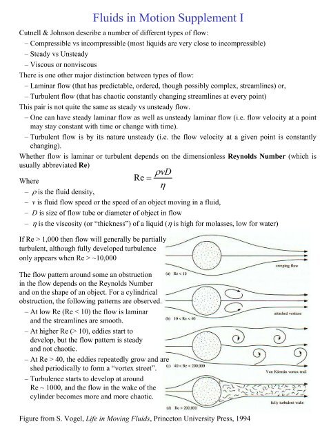
Cutnell & Johnson describe a number of different types of flow:
– Compressible vs incompressible (most liquids are very close to incompressible)
– Steady vs Unsteady
– Viscous or nonviscous
There is one other major distinction between types of flow:
– Laminar flow (that has predictable, ordered, though possibly complex, streamlines) or,
– Turbulent flow (that has chaotic constantly changing streamlines at every point)
This pair is not quite the same as steady vs unsteady flow.
– One can have steady laminar flow as well as unsteady laminar flow (i.e. flow velocity at a point
may stay constant with time or change with time).
– Turbulent flow is by its nature unsteady (i.e. the flow velocity at a given point is constantly
changing).
Whether flow is laminar or turbulent depends on the dimensionless Reynolds Number (which is
usually abbreviated Re)
Where
Re =
ρvD
η
– ρ is the fluid density,
– v is fluid flow speed or the speed of an object moving in a fluid,
– D is size of flow tube or diameter of object in flow
– η is the viscosity (or “thickness”) of a liquid (η is high for molasses, low for water)
If Re > 1,000 then flow will generally be partially
turbulent, although fully developed turbulence
only appears when Re > ~10,000
The flow pattern around some an obstruction
in the flow depends on the Reynolds Number
and on the shape of an object. For a cylindrical
obstruction, the following patterns are observed.
– At low Re (Re < 10) the flow is laminar
and the streamlines are smooth.
– At higher Re (> 10), eddies start to
develop, but the flow pattern is steady
and not chaotic.
– At Re > 40, the eddies repeatedly grow and are
shed periodically to form a “vortex street”.
– Turbulence starts to develop at around
Re ~ 1000, and the flow in the wake of the
cylinder becomes more and more chaotic.
Figure from S. Vogel, Life in Moving Fluids, Princeton University Press, 1994

Fluids in Motion Supplement I
Viscosity:
– SI units of viscosity, η = kg m -1 s -1 or Pa·s (cgs unit: Poise, P = g cm -1 s -1 = 0.1 Pa s)
– Viscosity varies with Temperature
Material
Viscosity (Pa·s)
Air (20 C): 0.000018
Water (20°C):
0.001 Pa s (=1 cP)
Water (40°C): 0.00065
Ethanol: 0.0012
Methanol: 0.00058
Glycerin (0°C): 12.0
Glycerin (30°C): 0.629
Oil, Olive (20°C): 0.084
30% aqueous Sucrose: 0.003
Molasses (45-50% Sucrose) 0.005-0.010
70% aqueous Sucrose: 0.481
Example S1 Reynolds Number for a baseball pitch
Baseball pitchers can routinely throw baseballs at speeds of 90 mph (40.2 m/s). The diameter of a
baseball is supposed to be 7.37 cm1.8 x 10 -5 Pa·s. The density of air is 1.29 kg/m 3 and the viscosity
of air is 1.8 x 10 -5 Pa·s.
a) What is the Reynolds Number for a fastball?
b) Will the flow past the ball be laminar or turbulent?
Reasoning: This is a straight plug-in problem using the definition of Reynolds Number. From the
notes on the previous page, the definition of Reynolds number is:
ρvD
Re =
η
where
ρ is the fluid density (not the baseball density),
v is speed of the air around the baseball, or, equivalently for the baseball problem, the speed of
the baseball through the air
D is diameter of the baseball (given as 7.37 cm)
η is the viscosity of the air (from the information given, η = 1.8 x 10 -5 Pa·s).
Solution:
a) The Reynolds number can be calculated using the values above:
3
ρvD (1.29 kg/m )(40.2 m/s)(0.0737 m)
Re = = = 2.12×
10
-5
η
1.8× 10 kg/(m ⋅s)
b) Since Re is 212,000, which is much greater than 1000 (the Reynolds Number above which flow
becomes turbulent) the flow around the baseball will be turbulent.
5

Fluids in Motion Supplement I
Some examples of Reynolds Numbers for biological organisms moving through fluids (air or water)
are shown in the table below. These values were calculated in much the same way as for the
baseball, but they use very rough estimates for the size of the organisms.
A large whale swimming at 10 m/s 300,000,000
A duck flying at 20 m/s 300,000
A large dragonfly moving at 7 m/s 30,000
Flapping wings of the smallest flying insect 30
An invertebrate larva, 0.3 mm long, at 1 mm/s 0.3
A sea urchin sperm moving at 0.2 mm/s 0.03
A bacterium, swimming at 0.01 mm/s 0.00001
(From S. Vogel, Life in Moving Fluids, Princeton University Press, 1994, Table 5.1)
One can find the size of the whale implied by the first item in the table above from the definition of
the Reynolds Number. If Re = 3 x 10 8 , then using values for the density of water from Table 11.1 in
Cutnell & Johnson (ρ water = 1000 kg/m 3 ) and the viscosity of water from the table on the previous
page of this supplement (η water = 0.001 Pas):
8
Re η (3× 10 )(0.001 kg/(m ⋅s))
D = = = 30 m
3
ρv
(1000 kg/m )(10 m/s)
A size of 30 m is consistent with the length of a large whale. For a complex shape like a whale the
size scale to use in the calculation of the Reynolds Number is a matter of debate, even among
experts. It is not always clear whether one should one set D equal to the width of the whale, or the
length of the whale, or the height of the whale (or some combination of the three). In most cases,
however, the Reynolds Number will not change enough to affect what type of flow (laminar or
turbulent) is predicted by the Re value if the width of the whale is used instead of the length. The
true flow pattern can only be found by experiment or from the study of scale models in wind or
water tunnels.
The idea that if Reynolds Number is the same for two objects of different sizes, flow patterns will be
the same leads to the idea of dynamic similarity. This implies that one can measure the flow
pattern for a scale model of an object in a wind tunnel and expect that the flow pattern around the
full-sized object will be similar if the density, viscosity or speed of the wind tunnel fluid are
adjusted to give the same Reynolds Number as the full-sized object.

Poiseuille Flow (Low Re flow in Tubes)
Jean Poiseuille (1797-1869), a medical doctor, studied flow in circular tubes at low Reynolds
number in order to understand the flow of blood in arteries, capillaries and veins. He found that
thanks to viscosity (which can be thought of as friction between layers of fluid), flow is fastest at
the tube center-line and the flow velocity is zero at the tube wall.
To visualize flow in tubes, look at Fig. 11.37 in Cutnell & Johnson and imagine concentric
cylinders of fluid at different distances, r, from the centerline in a tube of radius R. If one looks a
a cross section down the length of the tube, the flow profile (or velocity, v(r), as a function of
distance from the centerline) is a parabola, as shown in the figure at the bottom of this page. The
parabolic flow velocity profile can be summarized with the following equation:
⎛
v= v ⎜1−
r
⎝ R
At the tube wall, where r = R, one gets that v = v max (1 – R 2 /R 2 ) = v max (1 – 1) = 0. At the tube
centerline where r = 0, one gets that v = v max . It can be shown that the v max is:
max
The AVERAGE fluid velocity, turns out to be just half v max :
v
v
This is important since the total flow rate (used in the equation of continuity is related to the
AVERAGE velocity, not the maximum.
Rearranging this equation, we get the equation at Cutnell & Johnson call Poiseuille’s Law. Other
books call it the Poiseuille-Hagen Law to acknowledge the co-discoverer:
2
max 2
2
R ∆P
=
4η
L
⎞
⎟
⎠
2
1 R ∆P
= vmax
=
2 8η
L
2
2
⎛ R ∆P⎞
Q= Atube
v = ( π R ) ⎜ ⎟
⎝8η
L ⎠
4
π R
Q =
8η
∆P
L
R
r
v(r)
centerline
v max

Drag on an Object
Bernoulli’s Law describes the lift on an object fairly well (i.e. the pressure difference between the
top and bottom of an object in flow). It does not do so well for the drag on an object.
Bernoulli’s law applies for “ideal fluids” (i.e. fluids with zero viscosity), but neither air nor water
(the most common fluids encountered on the earth’s surface) are ideal fluids. Both have viscosity
that produces frictional drag. This adds a non-conservative work term to the conservation of energy
formulation that underlies Bernoulli’s Law. Thanks to viscosity, work has be done to get fluids to
move around objects and this leads to a pressure difference between the front and back of the object
(relative to the flow). Drag is caused by this difference in pressure between the front and back of an
object.
Experiments show that the drag force, F d , on an object will depend on:
– Area and shape of the object
– Speed with which the object moves relative to fluid
– Density of the fluid
– Reynolds Number
The standard procedure to calculate drag on an object is to use a modified form of Bernoulli’s Law
to find the force from the Bernoulli Pressure. For a spherical particle in flow, if A is the crosssectional
area of the object and ½ρv 2 is the Bernoulli Pressure at the front of the object (where v is
the object’s speed relative to the fluid), then the drag force will be:
⎛1
⎞
= ⎜ ⎟
⎝2
⎠
2
Fd
A ρv Cd
We put in a new factor, C d the drag coefficient, to take into account the viscous losses.
Drag coefficient changes with Reynolds Number and is different for differently shaped objects
Drag coefficients can be measured in wind tunnel tests or they can be calculated (using computers
to solve the extremely complex equations of hydrodynamics).
If the object in question is a sphere, experiments show that for high Re (>~1000):
C ≈ 0.44
d
So the drag equation for a sphere of radius R (where the cross-sectional area is πR 2 ) at high Re
becomes:
⎛1
Fd
R v
⎝2
2 2
= π ⎜ ρ ⎟
( 0.44)
Example S2 Drag on the baseball in Example S1
This equation would apply, for example, to the baseball in Example S1, for which Re ~200,000. For
this v = 40.2 m/s. The diameter of a baseball is supposed to be 7.37 cm, so the radius of the ball is
(0.0737 m)/2 = 0.0368 m. The density of air is 1.29 kg/m 3 so:
2⎛1 2⎞
2 1
3 2
Fd
= πR ⎜ ρv
⎟( 0.44 ) = π(0.0368 m) (1.29 kg/m )(40.2 m/s) ( 0.44)
= 1.95 N
⎝2 ⎠
2
⎞
⎠

Fluid Drag at Low Reynolds Number
For very low Reynolds Number (Re < 0.1 – this regime is called creeping flow), the drag
coefficient for a sphere has been shown to be:
C
d
=
24
Re
where Re is the Reynolds Number = Dvρ/η. Plugging this into the drag equation on the previous
page, and using the cross-sectional area of a sphere
⎛1 2⎞ 2⎛1 2⎞
24
Fd
= A⎜ ρv ⎟Cd
= πR ⎜ ρv
⎟
⎝2 ⎠ ⎝2 ⎠ 2 /
(note that D = 2R has been used here). There is a lot of cancellation and we get the final
expression for the Stokes drag, or drag on a sphere at very low Reynolds Number:
Fd
= 6πη
Rv
This expression was calculated by Stokes in 1850 for the drag force on a sphere of radius R
moving with speed v relative to a medium with viscosity η. This expression only applies to a
sphere, but other shapes have drag forces that have similar forms at low Reynolds Number.
Objects with densities ρ 1 that differ from the density, ρ 2 , of the surrounding medium will either
sink (if ρ 1 more dense than ρ 2 ) or float (if ρ 1 less dense than ρ 2 ).
For objects sedimenting in fluids three forces acting on the particle:
– Gravity, F g = mg = ρ 1 Vg
– Buoyant force, F b = m fluid displaced g = ρ 2 Vg
– Hydrodynamic drag, F d
( Rvρ η)
Sedimentation and Terminal Velocity
The drag force increases with speed and so if a particle starts at rest, it will accelerate until the
drag force equals the sum of the gravitational and buoyant forces. At this point the object will
move with a constant velocity. Choosing down to be negative, the force balance is then:
∑ Fy = Fd + Fb − Fg
= 0 F d F b
Plugging in for F g and F b , we get:
F + ρ gV − ρ gV =
d
2 1
0
ρ 1
ρ 2
We can rearrange to get the fluid drag at terminal velocity is given by:
Fd
( ρ ρ )
= −
1 2
gV
F g

Sedimentation of a Sphere at high Re
Suppose a spherical object with density ρ 1 is sinking (or floating) within a fluid. At high
Reynolds Number, the drag force is given by the modified Bernoulli drag:
2⎛1
2⎞
Fd
= πR ⎜ ρ
fluidv
⎟
⎝2
⎠
Plugging this into the sedimentation force balance on the previous page and using the formula for
the volume and area of a sphere:
2 1 2 4 3
πR ⎛ ⎜ ρ2v ⎞ ⎟( 0.44) = ( ρ1−ρ2)
g ⎛ ⎜ πR
⎞
⎟
⎝2 ⎠ ⎝3
⎠
There is a lot of cancellation here and one may then solve for the terminal velocity of the
sedimenting sphere.
v
8 Rg ⎛ ρ − ρ ⎞
g
⎝ ⎠
1 2
= ⎜ ⎟
3 C d
ρ2
( 0.44)
Example S3 Sinking speed of a cannonball in water
Suppose you have a 3 kg iron cannonball sinking in water. What is its terminal velocity?
First, find the radius of the cannonball. Since the density of iron is 7860 kg/m 3 :
So:
Since this radius is fairly large and the sinking speed (which we know from experience) will be
reasonably large, say 1 m/s, the Reynolds number = Dvρ/η ~ (2*0.045)(1)(1000)/(.001) ~ 90,000.
One can thus use the high Re formula for sedimentation:
v
We finally get:
R
cannonball
8 Rg ⎛ ρ −ρ
⎞ 8 (0.0450)(9.80) ⎛7860 −1000
⎞
⎜ ⎟ ⎜ ⎟
3 ⎝ ⎠ 3 (0.44) ⎝ 1000 ⎠
1 2
= =
Cd
ρ2
m 4 V
3
cannonball π R
cannonball
ρ = = 3
= 3m
33.00 ( kg)
3 3
0.0450 m
3
4πρ
= 4π
7860 kg/m
=
( )
v = 4.28 m/s

Sedimentation of a Sphere at low Re
Suppose a spherical object with density ρ 1 is sinking (or floating) within a fluid. At low Reynolds
Number, the drag force is given by the Stokes drag, so:
F d
= 6πηRv
Plugging this in and using the formula for the volume of a sphere:
4
6πη π ρ ρ
3
( )
3
Rv= R
1−
2
g
There is only a little cancellation and one may then solve for the terminal velocity of a sphere
sedimenting if the Reynolds Number is less than 1.
v =
2
9
R
2
( ρ − ρ )
1 2
η
g
Example S4 Sedimentation time for a cell in water
Suppose you have a red blood cell with an effective radius of 4 µm and density 1.15 g/cm 3
sedimenting in salt water that has a density of 1.05 g/cm 3 . How long will the cell take to
sediment a vertical distance of 5 cm?
Reasoning: Since the radius of the RBC is in the micrometer range, and we guess from
experience that the sedimentation speed is small (guess 1 mm/s) the Reynolds number = Dvρ/η ~
(2*4 x 10 -6 )(1 x 10 -3 )(1050)/(0.001) ~ 0.0084. This is very much less than 1 so we can use the
Stokes drag formula above:
2
−6
( ρ − ρ ) g ( × ) ( − )
2
2 R
4 10 1150 1050 (9.80)
1 2 2
v = =
9 η 9 (0.001)
v = ×
−6
3.5 10 m/s
So now we can use the definition of speed v = ∆x/∆t (here, v = h/t) to find the time to settle 5 cm
(= 1 x 10 -2 m):
t
h 0.05 m
= = = ×
−6
v 3.5×
10 m/s
4
1.4 10 s = 239 min = 4.0 hr