Review of Newtonian Mechanics - vol. II - Physics

Review of Newtonian Mechanics - vol. II
Aditya Joshi
October 7, 2005
Abstract
Volume II of A Review of Newtonian Mechanics begins with the special
case of uniform circular motion, segueing into a more general discussion
of uniformly accelerated circular motion. The latter is presented in close
analogy to the discussion of straight-line motion in volume I. The reader
is encouraged to note the many similarities between the two. The theorems
of conservation of momentum and energy are simply stated since
we implicitly discussed these in vol.I. We end this two-part article with a
miscellany of useful mathematics, including a table of useful derivatives
and integrals and a (very optional, but quite interesting) discussion on
finding averages of continuous functions. This may however, illuminate
some otherwise confusing aspects on AC circuits in Phy 8B.
• Disclaimer: This document is purely for self-edification. It is not
meant as a formula sheet for an exam, nor is it meant to be selfcontained
(although I have tried to make it so) or for that matter,
complete. I have tried my best to make sure that no conceptual
errors reside herein. Typos are a different matter altogether...
Contents
Volume II: Rotation, the Conservation Theorems and miscellaneous
useful mathematics 3
1 The problem of uniform circular motion UCM 3
Statement of the problem . . . . . . . . . . . . . . . . . . . . . . 3
1.1 Finding the acceleration of the body . . . . . . . . . . . . . . . . 3
Why is the acceleration “centripetal”? . . . . . . . . . . . . . . . 3
The limit t 1 → t 2 (or ∆t → 0) . . . . . . . . . . . . . . . . . . . 5
Finding the angular velocity ω . . . . . . . . . . . . . . . . . . . 5
1.2 Whence the Centripetal Force? . . . . . . . . . . . . . . . . . . . 6
2 Uniformly accelerated circular motion (ACM ) 7
2.1 Axial vectors (or pseudo-vectors) . . . . . . . . . . . . . . . . . . 8
2.2 Angular position (θ) and angular displacement ( ∆θ) ⃗ . . . . . . . 9
1

2.3 Angular velocity (⃗ω) . . . . . . . . . . . . . . . . . . . . . . . . . 10
2.4 Angular acceleration (⃗α) . . . . . . . . . . . . . . . . . . . . . . . 10
2.5 Torque (⃗τ) and “Newton’s 2 nd law” analogue for rotation . . . . 10
2.6 The Kinematic equations for constant angular acceleration . . . . 11
3 Calculating torque in physics problems 11
3.1 Method 1 - vector method . . . . . . . . . . . . . . . . . . . . . . 11
3.2 Method 2 - scalar method . . . . . . . . . . . . . . . . . . . . . . 13
4 The Conservation Theorems 14
4.1 Momentum conservation . . . . . . . . . . . . . . . . . . . . . . . 14
4.2 Energy conservation (now that’s a thought) . . . . . . . . . . . . 15
5 Useful math formulae 15
5.1 Commonly used derivatives in elementary physics . . . . . . . . . 15
Differentiation Rules . . . . . . . . . . . . . . . . . . . . . . . . . 15
Derivatives . . . . . . . . . . . . . . . . . . . . . . . . . . . . . . 15
5.2 Commonly used integrals in elementary physics . . . . . . . . . . 16
Integration Rules . . . . . . . . . . . . . . . . . . . . . . . . . . . 16
Integrals . . . . . . . . . . . . . . . . . . . . . . . . . . . . . . . . 16
Averages of functions . . . . . . . . . . . . . . . . . . . . . . . . . 16
Average values of cos 2 x and sin 2 x over the interval [0, 2π] . . . . 17
2

1 The problem of uniform circular motion UCM
We will state this problem in a very simple way. Please note the logical order in
which we proceed here. Specifically, note that we initially make no assumptions
about forces acting on the body. Rather, we impose a certain kind of motion
on the body and then proceed to calculate the kind of force necessary in order
to create this motion. The centripetal force will arise naturally and will be
born of necessity.
Statement of the problem
A body of mass M is constrained to move in a circle of radius R at a constant
speed | −→ v | = v. It is vital that you realize that it is only the speed (v) which
is constant. The direction of the velocity vector must be continually changing
in order to stay on the curved path. The problem is to find the force needed to
create this physical situation.
Newton’s 2 nd Law (Vol.I, eq.5) relates the force to the acceleration by:
−→ F = M · −→ a (1)
Therefore, if we can find the acceleration that the body undergoes, eq.( 1)
immediately tells us how much force is required (and in what direction) in order
to keep the body moving in a circle.
Since the velocity vector is changing with time (just the direction), the body
is — by definition — undergoing an acceleration −→ a , which we wish to calculate
(well...at least I do).
1.1 Finding the acceleration of the body
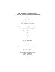
We begin by drawing a detailed sketch of the motion at two instants of time very
close to each other (see fig. 1). The time difference is ∆t = t 2 −t 1 . The velocities
at the two points of time are v 1 and v 2 and they are directed tangential to the
circle. The direction of the velocity at any point on the circle is the direction
the body is travelling at that instant.
Why is the acceleration “centripetal”?
To find the change in velocity ( −→ ∆v = −→ v 2 − −→ v 1 = −→ v 2 + (− −→ v 1 )), we just have to find
the vector sum of −→ v 2 and (− −→ v 1 ). This is shown explicitly in fig. 1. Because of the
symmetry (the fact that both vectors have the same length (same magnitude of
the velocity)), the vector sum (thick green arrow) is seen to point towards the
center of the circle. It will do so for any pair of points on the circle. The vector
sum is the change in velocity and so −→ ∆v points towards the center all the time.
Now, the average acceleration between points 1 and 2 is just the rate at
which the (vector) velocity is changing.
−→
−−→ ∆v
a avg(1→2) =
(2)
∆t
3

Figure 1: (a) Snapshot of motion at two times t 1 and t 2 very close to each other.
(b) Finding ⃗ ∆v visually.
So, the acceleration vector just inherits the direction from −→ ∆v. Therefore,
the acceleration is “centripetal”, which means “center-seeking”. The radial unit
vector (a direction vector that always points away from the center of the circle)
is denoted by ˆr. So, we can denote the direction of the acceleration by −ˆr.
To find −→ ∆v, note that the horizontal components of −→ v 2 and − −→ v 1 cancel each
other and the vertical components add in the centripetal direction (the −ˆr direction).
From the geometry, the vertical components are each equal to v cos(φ).
So, we get:
−→
∆v = −→ v 2 + (− −→ v 1 )
= (v cos(φ) + v cos(φ)) (−ˆr)
= 2 v cos(φ)(−ˆr) = 2 v cos( π 2 − ∆θ )(−ˆr) . . . . . . which finally becomes :
2
−→
∆v = −2 v sin( ∆θ )ˆr (3)
2
So, the average acceleration can be written as:
4

−−→
a avg(1→2) =
−→
∆v
∆t
∆θ
2 v sin(
The limit t 1 → t 2 (or ∆t → 0)
2 )
= − ˆr . . . (from eq. 3)
∆t
∆θ
sin(
2
= −2 v ) ( ∆θ
2 )
( ∆θ
2 ) ˆr . . . (just the usual trick)
∆t
[
sin(
∆θ
2
= − v
)
] [∆θ
( ∆θ
2 ) ∆t
]
ˆr (4)
If the two instants of time are taken to be very close, then the angle ∆θ becomes
very very small. The average acceleration (from eq. 4— in the limit that ∆t → 0
and ∆θ → 0 (and t 1 → t 2 ))— becomes the instantaneous acceleration at time
t 1 :
But,
Also,
−→ a (t1 ) = − v Limit
} {{ }
(∆θ→0)
[
sin(
∆θ
2 )
]
( ∆θ
2 )
Limit
} {{ }
(∆t→0)
[ ] ∆θ
ˆr (5)
∆t
[
sin(
∆θ
2
Limit
)
]
} {{ } ( ∆θ
(∆θ→0)
2 ) = 1 . . . (from calculus) (6)
[ ] ∆θ
Limit
} {{ }
= dθ
∆t dt = ω (7)
(∆t→0)
Where, ω (pronounced ‘omega’)is the angular velocity of the body, i.e.
the amount of angle (in radians) swept out by the body per unit time, i.e. the
rate of change of angular position with respect to time.
Using eq. 6 and eq. 7 in eq. 5, and generalizing t 1 to any time t, we obtain:
[ ]
−→ dθ
a (t) = −v · 1 ˆr = −v ω ˆr (8)
dt
Finding the angular velocity ω
We can use a very obvious fact here. The time taken (T) for the body to sweep
out an angle 2π (i.e. the whole circle of radius R) at an angular speed ω should
be the same as the time taken for it to cover the entire circumference (C = 2πR)
5

at (linear) speed v. That’s quite a mouthful, so you might want to read it again.
Since time = distance angle covered
speed
=
angular speed
, we have:
T = 2π ω = 2πR
v
Simplifying this gives the very useful relation:
ω = v R
(9)
Using eq. 9 in eq. 8 and noticing that the acceleration is constant in time,
we finally obtain a formula for the centripetal acceleration of the body:
−→ −v 2
a = ˆr (10)
R
Along the way, we also define a useful quantity called frequency. The
period of rotation was defined as the time (T) it took to move once around
1
the circle. So,
T
would mean the number of rotations made per second. This
is the frequency (f). (Sometimes, you may find it denoted by the Greek letter
[ν], pronounced ‘nu’ ). Refer back to eq. 9.
f = 1 T = ω 2π =
v
2πR
(11)
1.2 Whence the Centripetal Force?
Now, we are ready to answer the most important part of the problem — what
kind of force is neeeded to make a body go in a circle at a constant speed v?
Applying Newton’s 2 nd Law (eq. 1) to our rotating body, we obtain:
So,
−→ F = M
−→
( a
) −v
2
= M
R ˆr . . . (using eq. 10)
)
−→ F =
(−M v2
ˆr (12)
R
So, eq. 12 tells us that the force that causes this motion (constrained along
a circle of radius R and travelling at constant speed v) must be directed towards
the center of the circle and must have magnitude M v2
R
. This is the origin of the
term “centripetal force”.
We have merely figured out how much force is needed. We have said nothing
about where this force actually comes from. Well...it could come from anywhere!
The origin of the force could be a person holding a stone on a string and twirling
it round (F cp = T ension in string). Or, such a force could come from injecting
a charged particle into a region of uniform magnetic field. Then, the centripetal
force is provided by the magnetic force acting on the particle.
6

At this point, you may find it instructive to calculate all relevant quantities
for the magnetic field example mentioned above. In particular, find the necessary
centripetal force for a particle of mass M to move in a circle of radius R at
constant speed v and set it equal to the magnetic force acting on the particle (of
charge q) in a uniform magnetic field B along the Z-axis. If the initial velocity of
the particle before it sees the B-field was along the X-direction, the subsequent
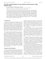
motion of the charge is confined to the XY-plane. If the initial velocity of the
particle has a component along the Z-direction (i.e.
−→ v0 = v 0xˆx + v 0z ẑ), then
only v 0x will be seen by the B-field and v 0z will stay unaffected. So, the particle
will move in the Z-direction along a straight line with constant speed v 0z and it
will move in circles in the different XY-planes. The motion taken together will
then look like a helix (the mathematical name for a ‘corkscrew’) with its axis
along Z (See fig. 2).
Figure 2: Path of a charged particle injected at an angle to a uniform magnetic
field along the Z-direction.
2 Uniformly accelerated circular motion (ACM )
We have seen the case of a body rotating at a constant angular velocity in the
previous section. It is only natural to ask how this body was set into rotation
in the first place. It must have been at rest at some time in the past and some
7

agency must have acted upon it to make it rotate at some non-zero angular
velocity now. We will use the same logic that we used in vol.I and consider
that agency the cause and call it the Torque ( −→ τ ). The effect, as usual will be
called the acceleration (the change in velocity). Only, here we have an angular
velocity, so the corresponding acceleration will be angular acceleration ( −→ α ).
The angular velocity is also a vector ( −→ ω ).
We haven’t been very clear so far about what we mean by the directions of
these vectors ( −→ τ , −→ α and −→ ω ). We shall attept to clarify that point now.
2.1 Axial vectors (or pseudo-vectors)
The three vectors mentioned above are part of a class of mathematical objects
called pseudo-vectors or axial vectors. The first name conveys the fact
that while they may have a magnitude and direction, they are not honest-togoodness
vectors in the technical sense of the word. Even if we forgetting about
the technical point, there is the fact that these pseudo-vectors do not really do
anything along the direction that they point in. So, for instance, the direction
of the angular velocity is not the direction in which the body actually moves.
How then are we to interpret the direction? Well, the second name gives
us the answer. The direction of an axial vector defines an axis around which
the effects actually occur as well as the orientation (i.e. clockwise (CW) or
counterclockwise (CCW) around the axis). The last part is given by the right
hand curl rule (henceforth denoted as RHCR— put your thumb in the direction
of the axial vector and the curling of the fingers defines the orientation implied
by the vector.
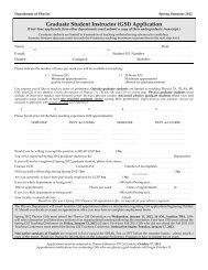
Figure 3: Angular velocity as an axial vector. Also shown: 2 points on the
circle (with position vectors r 1 andr 2 ) where the body has velocity v 1 and v 2
respectively.
Let’s take an example. Consider the uniformly rotating body from the previous
section (see fig. 3). Since the body is rotating CCW, we can use the RHCR
8

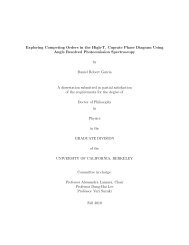
Figure 4: Angular coordinates of a point and angular displacement.
in reverse — the curled fingers point CCW and the thumb then points out of the
page (towards you) — to get the direction of the axial vector, i.e. the angular
velocity vector −→ ω . Note the conventions for denoting the “into the page” and
“out of the page” directions shown in the figure.
At this point, you may question the necessity of axial vectors. Why not just
call the angular velocity CW or CCW and be done with it? The main reason
is convenience. By defining these quantities as vectors, we can work with them
exactly as we have worked with other vectors so far. We can write laws and
equations that are very general by using the fact that these things are vectors.
For example, the relationship (see eq. 9) between the instantaneous linear
velocity ( −→ v ) of the particle moving in a circle which is presently at a position
vector −→ r and its angular velocity ( −→ ω ) is written succinctly as:
−→ v =
−→ ω ×
−→ r (13)
Try the right hand rule for cross-products at each of the 2 points in fig. 3
and see if you get the correct magnitude and direction for the velocity. The
following subsections should illuminate this a little more.
2.2 Angular position (θ) and angular displacement ( ⃗ ∆θ)
We can denote a point on the circle by a position vector −→ r pointing from the
origin to the point (see fig. 4). Then, the position of the point can also be
denoted by the angular position as measured from some reference axis. If
we agree to measure all our angles CCW from the +X-axis as shown, then the
point-1 has an angular position −→ θ 1 . What does the vector sign mean here? The
same as before — a positive θ means that we should go an angle of θ 1 CCW
from the +X-axis to get to point-1.
Angular displacement is then just the difference of two angular positions:
−→
∆θ 1→2 = −→ θ 2 − −→ θ 1 (14)
9

Again, the direction of the displacement vector is just the sense (CW or
CCW) of the displacement by the RHCR (right hand curl rule).
Units: Angle is measured in radians (rad). 1 circle = 360 ◦ = 2π rad. Note
that ‘rad’ is just a convenient placeholder and angle has no real units. So, ‘rad’
is sometimes dropped at will.
2.3 Angular velocity (⃗ω)
Angular velocty measured the rate at which the angular position of a body
changes with time. The same direction conventions apply.
−→ ω =
d −→ θ
dt
(15)
Units: Angular velocity would be rad
s
in SI units.
2.4 Angular acceleration (⃗α)
Angular acceleration (α - pronounced ‘alpha’) is just the rate at which the
angular velocity is changing. For instance, suppose a body is initially at rest
(ω = 0) and it starts moving at 1 rad
s
after the first sec. and at 2 rad
s
after
the second sec. and so on. This means that it is accelerating at the rate of
rad
persec. or at the rate of 1
1 rad
s
s 2 .
2.5 Torque (⃗τ) and “Newton’s 2 nd law” analogue for rotation
Just as we need some agency to make things accelerate in linear mechanics
(vol.I), we need some agency or some ‘cause’ to get things to accelerate in
the angular sense. This agency is called Torque (τ - pronounced ‘tau’). Unit:
Newton · meter (N · m).
So, we can say that a torque produces an angular acceleration. This relationship
can be written in the fashion of Newton’s 2 nd Law:
−→ τ ∝
−→ α
The proportionality constant is the rotational analogue of mass and is called
the moment of inertia (I [note that this not current]). Just as mass dictates
how easy or difficult it is to change the motion of a body (i.e. accelerate it), so
the moment of inertia dictates how easy or difficult it is to change the rotation
of a body. For the case of a single point mass M rotating around a circle or
radius r, the moment of inertia is I = M r 2 . For a full discussion on moments
of inertia, please consult a good elementary physics textbook. Units: kg m 2 .
Then, we have:
−→ τ = I
−→ α (16)
This is “Newton’s 2 nd law” for rotation.
10

2.6 The Kinematic equations for constant angular acceleration
For a constant angular acceleration (produced by a constant torque), the angular
position and angular velocity can be calculated in the same way that we
calculated them for linear motion in vol.I (eqs.18 there). So, I will present in
Table. 1, the final equations, comparing them to the kinematic equations for
straight line motion. Also included in the table are all the basic quantities in a
comparative format so that the reader may see the amazing similarity between
the relations.
3 Calculating torque in physics problems
Consider a rigid body skewered on the Z-axis such that it is free to rotate only
in the XY-plane about the Z-axis as shown in fig..
Further, consider a point ‘P’ on the body located at position vector −→ r . Here,
−→ r is a vector lying in the XY-plane with its tail at the Z-axis and its head on
the point P.
If a force −→ F is applied at the point P, the body will experience a torque −→ τ given
by:
−→ τ =
−→ r ×
−→ F (17)
Let us take an example where the Force and the point P are defined (in MKS
units) as follows:
−→ r = (2ˆx + 3ŷ) m
−→ F = (4ˆx − 2ŷ) N
There are 2 ways to evaluate the torque.
3.1 Method 1 - vector method
Here, we can use the direct definition of the vector torque from eq. 17. Before
we do that, we note some simple facts that can be easily verified by using the
right hand rule:
• ˆx × ŷ = ẑ
• ŷ × ẑ = ˆx
• ẑ × ˆx = ŷ
So, the simple rule to remember is that cross-products in the order x →
y → z → x are positive. Going in the other order gives negative results. For
11

Straight-line motion
Rotational motion
Important physical quantities and cross-relations
1) Mass: M Moment of inertia: I
2) Linear Postion: −→ r Angular position: −→ θ
3) Linear Velocity: −→ v Angular velocity: −→ ω = d−→ θ
dt
−→ v =
−→ ω ×
−→ r
4) Linear Acceleration: −→ a Angular acceleration: −→ α = d−→ ω
dt
−→ a tangential = −→ α × −→ r
(This points along the circular path. This is identically
zero for uniform circular motion where ω = constant).
−→ a centripetal = − v2
R ˆr = −R ω2ˆr
(This is the familiar centripetal acceleration. It will
change continuously if ω is changing).
5) Force: −→ F Torque: −→ τ
−→ τ =
−→ r ×
−→ F
(where ⃗r is the position of the point
of application of the force).
6) Linear momentum: −→ p = M −→ v Angular momentum: −→ L = I −→ ω
7) Newton’s 2 nd Law: “Newton’s 2 nd Law” for rotation:
−→ F = M
−→ a = M
d −→ v
dt
= d−→ p
−→
dt
τ = I
−→ α = I
d −→ ω
dt
= d−→ L
dt
Kinematic equations
(*) Linear acceleration a = constant. Angular acceleration α = constant
1) v(t) = v 0 + a · t ω(t) = ω 0 + α · t
2) x(t) = x 0 + v 0 · t + 1 2 a · t2 x(t) = θ 0 + ω 0 · t + 1 2 α · t2
3) v(t) 2 = v0 2 + 2 a (x(t) − x 0 ) ω(t) 2 = ω0 2 + 2 α (θ(t) − θ 0 )
Table 1: Kinematic quantities and equations
12

example, ŷ × ˆx = −ẑ.
Now, we can evaluate the torque using simple algebra:
−→ τ =
−→ r ×
−→ F
So,
= (2ˆx + 3ŷ) × (4ˆx − 2ŷ)
= (2)(4)(ˆx × ˆx) + (2)(−2)(ˆx × ŷ) + (3)(4)(ŷ × ˆx) + (3)(−2)(ŷ × ŷ)
= (2)(4)(0) + (2)(−2)(ẑ) + (3)(4)(−ẑ) + (3)(−2)(0)
= −4(ẑ) + 12(−ẑ) + (3)(−2)(0)
−→ τ = −16ẑN · m (18)
3.2 Method 2 - scalar method
First, we find the magnitude of the torque. Imagine the two vectors −→ r and −→ F
placed tail to tail (again, see fig.). Let θ be the smaller angle between them.
Then, the magnitude of the torque is given by the definition of the cross-product:
τ = | −→ τ | = | −→ r | ∣ −→ F ∣ sin θ
So, τ = r F sin θ (19)
The direction of a cross-product is given by the right hand rule as follows:
1. Hold your right palm flat with your thumb stretched away from the other
fingers (I feel like a fortune-teller).
2. Lay the fingers of your right hand along the first vector ( −→ r ) of the product
(order is important).
3. Reorient your palm in such a way that you can curl your 4 fingers towards
the 2 nd vector ( −→ F ) through the smaller angle (θ) between the 2
vectors.
4. The direction in which your thumb ends up pointing after this reorientation
is then the direction of the cross-product ( −→ τ ).
To calculate the magnitudes for our example above, we note:
r = −→ r = √ (2) 2 + (3) 2 m = √ 13 m (20a)
F = −→ F = √ (4) 2 + (−2) 2 N = √ 20 N (20b)
If the angle θ is not explicitly given (as in this example), you can use a
simple trick to find it. The dot-product of 2 vectors is −→ A • −→ B = A B cos θ. So,
the angle θ can be found as:
13

( −→A −→ )
• B
θ = cos −1 A B
(21)
This is easy to do because the dot-product has a simple form when you know
the vector components: −→ A • −→ B = A x B x + A y B y + A z B z . For our example, the
angle is:
( )
(2ˆx + 3ŷ) • (4ˆx − 2ŷ)
θ = cos −1 √ √
13 20
( )
2 · (4) + 3 · (−2)
= cos −1 √
260
( ) 2
= cos −1 √
260
θ = 82.87 ◦ (22)
Then, eq. 19 for the magnitude of the torque becomes (using eq. 20 and
eq. 22),
τ = r F sin θ
= √ 13 √ 20 sin(82.87)N · m
τ = 15.99 N · m (23)
The direction (from the detailed procedure given above - the right hand rule)
is “going into the page”, i.e. in the negative Z-direction. Compare this with
eq. 18.
Note that for our example, where the 2 vectors were given in unit-vector notation,
this was a really roundabout way of doing the problem. However, if you
are given the magnitudes of the two vectors and their relative angle, then this
would be the way to go. So, the two methods are really not free choices. You
should use the one that is most relevant to the problem as stated.
4 The Conservation Theorems
4.1 Momentum conservation
If the net force acting on a system is zero, then the system as a whole does
not accelerate. So, the velocity of the system as a whole (i.e. the velocity of
the center of mass of the system) does not change. Since the momentum (see
table 1) is: −→ p = M −→ v , the center-of-mass momentum also stays constant. So,
we immediately write the Theorem of Conservation of Momentum as:
For a system with no net external force acting on it, the total momentum of
the system (which is the vector sum of the momenta of all components of the
system) is a conserved quantity (i.e. is constant in time).
14

4.2 Energy conservation (now that’s a thought)
If no net force acts on a system, and if all the internal forces are conservative
(see the subsection on Potential Energy in Vol.I Section.3 for a definition of
conservative forces), then the total energy of the system is a conserved quantity.
5 Useful math formulae
5.1 Commonly used derivatives in elementary physics
Differentiation Rules
Here, f and g are both functions of x.
( df(g)
dg
d
df
(f + g) =
dx dx + dg . . . (Sum rule) (24)
dx
d
dg
(f · g)x = f ·
dx dx + g · df . . . (P roduct rule) (25)
dx
)
d
dx
( f
g
= g · df
dx − f · dg
dx
g 2 . . . (Quotient rule) (26)
d
df(g)
f(g(x)) = · dg(x) . . . (Chain rule) (27)
dx dg dx
In the chain rule above, just treat g as a simple variable in the first derivative
dg(x)
) and then treat it as a function of x in the second derivative (
dx ).
Ex. f(x) = e x and g(x) = x 2 . Then, f(g(x)) = e (g(x)) = e (x2) . Then, using
the chain rule, we obtain:
de (x2 )
dx
Derivatives
= deg
dg
· dg(x)
dx
= e g · dx2
dx
= e(x2) · (2x).
d
sin x
dx
= cos x (28)
d
cos x
dx
= − sin x (29)
d
dx tan x = sec2 x = 1
cos 2 x
(30)
d
)
dx
= a · e x (for a = some constant) (31)
d
dx xN = N · x N−1 . . . (for any N) (32)
d
dx (ln x) = 1 . . . (ln x is the natural log function)
x
(33)
15

5.2 Commonly used integrals in elementary physics
Integration Rules
Here, u and v are both functions of x.
∫
∫ ∫
(u + v)dx = udx + vdx . . . (Sum rule) (34)
∫
∫ ∫ ( ∫ ) du
(u · v)dx = u · vdx − vdx dx (Integration by parts)(35)
dx
If ∫ f(x)dx = g(x), then
∫
f(A · x + B)dx =
g(A · x + B)
A
. . . (F or A and B constant). (36)
Integrals
∫
dx(sin x) = − cos x (37)
∫
dx(cos x) = sin x (38)
∫
dx(e a·x ) = ex (for a = some constant) (39)
a
∫
dx (x N ) = xN+1
. . . (for any N except N = −1) (40)
N + 1
∫ ( 1
dx = ln x . . . (ln x is the natural log function) (41)
x)
Averages of functions
The average value of a function f(x) over a range x ∈ [x 1 , x 2 ] is denoted as 〈f〉
and defined as:
∫x 2
f(x)dx
x
〈f〉 =
1
∫x 2
dx
x 1
(42)
This is a useful formula for finding the averages of some important functions
that you will see in AC circuits.
16

Average values of cos 2 x and sin 2 x over the interval [0, 2π]
〈
cos 2 x 〉 =
2π ∫
(cos 2 x)dx
0
2π ∫
So, 〈 cos 2 x 〉 = 1 2
0
2π ∫
0
dx
(1+cos 2x)
2
dx
=
[x] 2π
0
[ x
] 2π
2 0
=
+ [ sin 2x
4
2π
= π + 0
2π
] 2π
0
(43)
(44)
In eq. 43, we used the trigonometric identity: cos 2 x =
A similar calculation gives:
(1+cos 2x)
2
.
〈
sin 2 x 〉 = 1 2
(45)
This ends Volume II of “A Review of Newtonian Mechanics”. I
hope this will prove useful. It certainly was a lot of fun to write!
17