Solar physics meeting at IIA, Bangalore
Solar physics meeting at IIA, Bangalore
Solar physics meeting at IIA, Bangalore

Create successful ePaper yourself
Turn your PDF publications into a flip-book with our unique Google optimized e-Paper software.
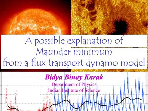
A possible explan<strong>at</strong>ion of<br />
Maunder minimum<br />
from a flux transport dynamo model<br />
Bidya Binay Karak<br />
Department of Physics<br />
Indian Institute of Science
Layout of the talk:<br />
‣Observ<strong>at</strong>ional fe<strong>at</strong>ures of Maunder<br />
Minimum.<br />
‣Building a flux transport Babcock-Leighton<br />
model.<br />
‣Find out the source of randomness in solar<br />
cycle.<br />
‣Use this model to explain the origin of<br />
Maunder Minimum.
Maunder minimum:<br />
‣Galileo's s Telescope invention in 1609.<br />
‣Maunder minimum period = 1645 to 1715 (Eddy,<br />
1976; Foukal, 1990; Wilson, 1994)<br />
‣68% of days were observed; sunspots appeared<br />
during 2% of the days (Hoyt & Sch<strong>at</strong>ten 1996)<br />
‣Rel<strong>at</strong>ed to little ice age.<br />
‣Cosmogenic isotopes: Be 10 and C 14
27 grand minima in last 11,000 years<br />
(from C 14 d<strong>at</strong>a by Usoskin et al. 2007)<br />
Do other stars show Maunder Minimum?<br />
Yes (Baliunas et al. 1995).<br />
Characteristics of Maunder Minimum:<br />
period from 1645-1670:<br />
Very few sunspot in two<br />
hemispheres.<br />
period from 1670-1715:<br />
Sunspots mostly on<br />
southern hemisphere<br />
(Ribes & Nesme-Ribes<br />
1993; Sokoloff & Nesme-<br />
Ribes 1994).
Usual 11-year period of<br />
solar activity (Schwab<br />
cycle) was continued.<br />
(Beer et al. 1998,<br />
Miyahara et al. 2004)<br />
1645 1680 1715<br />
years<br />
Sudden initi<strong>at</strong>ion but gradual recovery (Usoskin et al.<br />
2000)
• Induction equ<strong>at</strong>ion:<br />
∂<br />
B<br />
∂<br />
t<br />
= ∇ × ( v × B ) + η ∇ B<br />
2<br />
• Magnetic Reynolds Number:<br />
VB / L<br />
R Rm<br />
= =<br />
ηB/<br />
L<br />
2<br />
VL<br />
η<br />
• In Astrophysical systems, R m usually high, magnetic fields<br />
move with plasma – flux is frozen (Alfven, 1942).<br />
• Magnetoconvection (Chandrasekhar 1952, Weiss 1981) –<br />
convective region gets separ<strong>at</strong>ed into non-magnetic and<br />
magnetic space – the l<strong>at</strong>ter constitutes flux tubes.
Dynamo Model:<br />
Parker (1955)<br />
Axisymmetric magnetic field= toroidal+poloidal<br />
B = B ( r, θ<br />
) e φ<br />
+∇×<br />
[ A ( r, θ<br />
) e<br />
φ<br />
]
Toroidal Field Gener<strong>at</strong>ion (ω Effect)<br />
(Schou et al. 1998;<br />
Observ<strong>at</strong>ionally verified Charbonneau et al. 1999)
Poloidal Field Gener<strong>at</strong>ion:– The Mean Field α-<br />
effect/classical α-effect<br />
• Small scale helical convection – Mean-Field α-effect (Parker 1955)<br />
• Buoyantly yrising toroidal field is twisted by helical turbulent<br />
convection, cre<strong>at</strong>ing loops in the poloidal plane<br />
• The small-scale loops diffuse to gener<strong>at</strong>e a large-scale poloidal field
Towards flux transport dynamo<br />
• Induction equ<strong>at</strong>ion:<br />
model<br />
∂ B =∇× ( v × B)<br />
+ η ∇<br />
2<br />
B<br />
∂t<br />
t<br />
Evolution of mean (large scale) field is given by<br />
∂ B = ∇× ( v × B + α<br />
B ) + η<br />
2<br />
T<br />
∇<br />
B<br />
∂t<br />
•Our approach is kinem<strong>at</strong>ics (velocity field is given)
In axisymmetry case<br />
Velocity field= Ω ( r , θ ) r s in θ e + v re r + v e<br />
Toroidal field evolution:<br />
φ θ θ<br />
differential i rot<strong>at</strong>ion meridional circul<strong>at</strong>ion<br />
i<br />
B = Br (, θ) eφ<br />
+∇× [ Ar (, θ) eφ]<br />
∂ B<br />
1 ⎡<br />
∂ ∂<br />
⎤<br />
2<br />
1<br />
+ ( rvr B ) + ( vθ<br />
B ) = ηt ( ∇ − ) B + s ( B<br />
p. ∇Ω<br />
)<br />
2<br />
∂t r⎢<br />
⎣∂r ∂θ<br />
⎥<br />
⎦ s<br />
1 ∂ηt<br />
∂<br />
+ ( rB)<br />
r ∂ r ∂ r<br />
Poloidal field evolution:<br />
2<br />
∂A<br />
A<br />
1 1<br />
+ (. v ∇ )( sA) = η (<br />
2<br />
p ∇ − ) A + S<br />
∂t<br />
s s<br />
2<br />
α
Babcock–Leighton alpha effect: (Babcock 1961; Leighton 1969)<br />
S<br />
α<br />
=<br />
α<br />
B<br />
1 ⎡ r−r1 ⎤⎡ r−r2<br />
⎤<br />
0 θ<br />
1 +<br />
( ) 1 ( ) ith 0<br />
⎢<br />
erf<br />
⎥⎢<br />
erf<br />
⎥ 25 /<br />
1 2<br />
α = α cos θ 1 + ( ) 1 − ( ) with = 25 m/s<br />
4⎣ d ⎦⎣ d ⎦<br />
α
Transport mechanisms: 1) meridional circul<strong>at</strong>ion 2) diffusivity<br />
where,<br />
and<br />
α<br />
1<br />
0.9<br />
0.8<br />
0.7<br />
0.6<br />
0.5<br />
0.4<br />
0.3<br />
0.2<br />
0.1<br />
10 13<br />
10<br />
12<br />
10 11<br />
η p<br />
, η t<br />
10 10<br />
10 9<br />
0<br />
0.55 0.6 0.65 0.7 0.75 0.8 0.85 0.9 0.95 1 108<br />
r/R<br />
s<br />
S<br />
v ia θ<br />
s<br />
A s<br />
s
Magnetic buoyancy:<br />
y<br />
Inside flux Tube,<br />
P<br />
out<br />
B<br />
2µ<br />
2<br />
= P<br />
in<br />
+ out in<br />
P<br />
≤<br />
P<br />
Usually the inside is under-dense
Ch<strong>at</strong>terjee et al. (2004)
Fluctu<strong>at</strong>ion in polar field:<br />
Joy’s law: Tilts of bipolar<br />
sunspots increase with l<strong>at</strong>itude<br />
Sources of randomness:<br />
Sources of randomness:<br />
1. Fluctu<strong>at</strong>ions in the B–L process<br />
of poloidal field gener<strong>at</strong>ion
2. Fluctu<strong>at</strong>ion in the meridional circul<strong>at</strong>ion:<br />
Direct/Observ<strong>at</strong>ion study: (H<strong>at</strong>haway 1996;<br />
Snodgrass and Dailey 1996; Ulrich et al. 1988; Basu &<br />
Antia 2000; Haber et al. 2002; Gonz´alez-Hern´andez,<br />
et al. 2006; Gizon & Rempel 2008)<br />
Amplitude can vary from 1 m/s to 100 m/s.
Indirect/Theoretical study: (H<strong>at</strong>haway et al. 2003; Javaraiah &<br />
Ulrich 2006; Wang et al. 1991; Dikp<strong>at</strong>i & Charbonneau 1999;<br />
Nandy 2004, Ye<strong>at</strong>es et al. 2008 Wang et al. 2002)<br />
Amplitu ude of meridi ional circul<strong>at</strong>ion<br />
Period (yrs)
∂B<br />
1⎡<br />
∂ ∂ ⎤<br />
2 1<br />
+ ( rvrB) + ( vθ<br />
B) = η t( ∇ − ) B + s( Bp. ∇)<br />
Ω<br />
2<br />
∂ t r ⎣<br />
⎢<br />
∂ r ∂<br />
θ<br />
⎦<br />
⎥<br />
s<br />
1 ∂η<br />
t ∂<br />
+ ( rB) ⇒ ∆B ∝ s( Bp. ∇)<br />
Ω∆t<br />
r ∂<br />
r ∂<br />
r<br />
Amplitude of M.C. determines<br />
the strength of toroidal and also<br />
poloidal field<br />
Total suns spot numb ber<br />
Amplitude of meridional circul<strong>at</strong>ion
Flux transport dynamo combines three basic<br />
processes:<br />
(i) () strong toroidal field is produced by the stretching of<br />
the poloidal field => involves randomness.<br />
(ii) toroidal field rises due to magnetic buoyancy to<br />
produce sunspots and the decay of tilted bipolar<br />
sunspots produces poloidal field; =>involves<br />
randomness.<br />
(iii) poloidal field diffuses and advects by the<br />
meridional circul<strong>at</strong>ion first to high l<strong>at</strong>itudes and then<br />
down to the tachocline.
How to introduce fluctu<strong>at</strong>ion?<br />
The simplest way of doing is to change polar field<br />
randomly <strong>at</strong> each minima of solar cycle.<br />
To reproduce Maunder minimum:<br />
We propose th<strong>at</strong> the polar field <strong>at</strong> the beginning<br />
of the Maunder minimum fell to a very low value.<br />
1. we stop the code <strong>at</strong> a solar minimum.<br />
i<br />
2. Change the polar field in the following way:<br />
A N = 00A 0.0A N<br />
A S = 0.4A S<br />
3. we run the code for several cycles.<br />
Choudhuri & Karak (2009)
all<br />
Choudhuri & Karak (2009)
all<br />
Choudhuri & Karak (2009)
1.2<br />
Poloidal field in the solar wind<br />
1<br />
0.8<br />
0.6<br />
0.4<br />
0.2<br />
0<br />
−0.2<br />
1640 1650 1660 1670 1680 1690 1700 1710 1720 1730 1740 1750<br />
Year<br />
Sunspot eruption takes place only when the<br />
toroidal field reaches a value of 10 5 G.<br />
(Choudhuri 1998; D’Silva & Choudhuri 1993;<br />
Fan et al. 1993)<br />
During M.M., Babcock Leighton α effect will<br />
not work but Parker’s traditional mean field α<br />
effect will work.<br />
Choudhuri & Karak (2009)
Dynamo growth r<strong>at</strong>e is<br />
determined by the<br />
dynamo number,<br />
N<br />
D<br />
∝<br />
η<br />
α<br />
2<br />
P<br />
If the dur<strong>at</strong>ion of the M.M.<br />
is really an indic<strong>at</strong>or of the<br />
dynamo growth time, then<br />
it puts constraints on the<br />
parameters of the model.<br />
Choudhuri & Karak (2009)
Are we entering another grand<br />
minimum right now?<br />
Public<strong>at</strong>ion d<strong>at</strong>e of our paper:<br />
August, 2009<br />
Choudhuri & Karak (2009)
Are we entering another grand<br />
minimum right now?<br />
No!<br />
The polar field diminution factor γ <strong>at</strong> the<br />
end of 23 th cycle is 0.6 (Svalgaard,<br />
Cliver & Kamide 2000; Choudhuri,<br />
Ch<strong>at</strong>terjee & Jiang 2007) which is not<br />
sufficient to trigger a Maunder minimum.<br />
Choudhuri & Karak (2009)
Thank You
P<strong>at</strong>h between D to A can be advection domin<strong>at</strong>ed or<br />
diffusion domin<strong>at</strong>ed (Ye<strong>at</strong>es, Nandy & Mackey 2008)<br />
or can be turbulent pumping p domin<strong>at</strong>ed.