Towards a covariant formulation of electromagnetic wave polarization

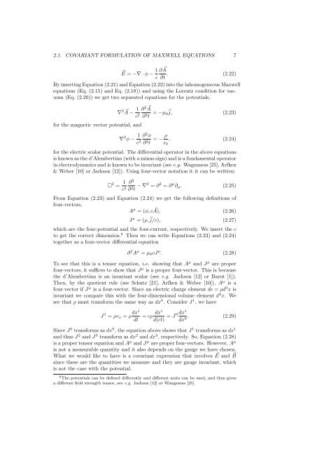
2.1. COVARIANT FORMULATION OF MAXWELL EQUATIONS 7
⃗E = −∇ · φ − 1 ∂A
⃗
c ∂t . (2.22)
By inserting Equation (2.21) and Equation (2.22) into the inhomogeneous Maxwell
equations (Eq. (2.15) and Eq. (2.18)) and using the Lorentz condition for vacuum
(Eq. (2.20)) we get two separated equations for the potentials,
for the magnetic vector potential, and
∇ 2 ⃗ A −
1
c 2 ∂ 2 ⃗ A
∂ 2 t = −µ 0 ⃗ j, (2.23)
∇ 2 φ − 1 c 2 ∂ 2 φ
∂ 2 t = − ρ ɛ 0
, (2.24)
for the electric scalar potential. The differential operator in the above equations
is known as the d’Alembertian (with a minus sign) and is a fundamental operator
in electrodynamics and is known to be invariant (see e.g. Wagnsness [25], Arfken
& Weber [10] or Jackson [12]). Using four-vector notation it it can be written:
□ 2 = 1 c 2 ∂ 2
∂ 2 t − ∇2 = ∂ 2 = ∂ µ ∂ µ . (2.25)
From Equation (2.23) and Equation (2.24) we get the following definitions of
four-vectors,
A µ = (φ, c ⃗ A), (2.26)
J µ = (ρ,⃗j/c), (2.27)
which are the four-potential and the four-current, respectively. We insert the c
to get the correct dimension. 8 Then we can write Equations (2.23) and (2.24)
together as a four-vector differential equation
∂ 2 A µ = µ 0 cJ µ . (2.28)
To see that this is a tensor equation, i.e. showing that A µ and J µ are proper
four-vectors, it suffices to show that J µ is a proper four-vector. This is because
the d’Alembertian is an invariant scalar (see e.g. Jackson [12] or Barut [1]).
Then, by the quotient rule (see Schutz [21], Arfken & Weber [10]), A µ is a
four-vector if J µ is a four-vector. Since an electric charge element de = ρd 3 x is
invariant we compare this with the four-dimensional volume element d 4 x. We
see that ρ must transform the same way as dx 0 . Consider J 1 , we have
J 1 = ρv x = ρ dx1
dt
= cρ dx1
d(ct) = J 0 dx1
dx 0 . (2.29)
Since J 0 transforms as dx 0 , the equation above shows that J 1 transforms as dx 1
and thus J 2 and J 3 transform as dx 2 and dx 3 , respectively. So, Equation (2.28)
is a proper tensor equation and A µ and J µ are proper four-vectors. However, A µ
is not a measurable quantity and it also depends on the gauge we have chosen.
What we would like to have is a covariant expression that involves ⃗ E and ⃗ B
since these are the quantities we measure and they are gauge invariant, which
is not the case with the potential.
8 The potentials can be defined differently and different units can be used, and thus gives
a different field strength tensor, see e.g. Jackson [12] or Wangsness [25].