Towards a covariant formulation of electromagnetic wave polarization

2.3. IRREDUCIBLE REPRESENTATION 17
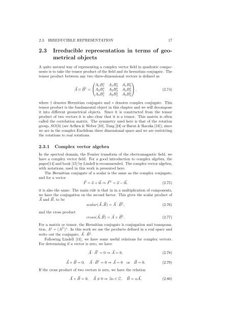
2.3 Irreducible representation in terms of geometrical
objects
A quite natural way of representing a complex vector field in quadratic components
is to take the tensor product of the field and its hermitian conjugate. The
tensor product between any two three-dimensional vectors is defined as
⎛
⃗A ⊗ B ⃗ † = ⎝ A ⎞
1B1 ∗ A 1 B2 ∗ A 1 B3
∗
A 2 B1 ∗ A 2 B2 ∗ A 2 B3
∗ ⎠ , (2.74)
A 3 B1 ∗ A 3 B2 ∗ A 3 B3
∗
where † denotes Hermitian conjugate and ∗ denotes complex conjugate. This
tensor product is the fundamental object in this chapter and we will decompose
it into different geometrical objects. Since it is constructed from the tensor
product of two vectors it is also clear that it is a tensor. This matrix is often
called the correlation matrix. The symmetry used here is that of the rotation
group, SO(3) (see Arfken & Weber [10], Tung [24] or Barut & Raczka [18]), since
we are in the complex Euclidean three dimensional space and we are restricting
the rotations to real rotations.
2.3.1 Complex vector algebra
In the spectral domain, the Fourier transform of the electromagnetic field, we
have a complex vector field. For a good introduction to complex algebra, the
paper[14] and book [15] by Lindell is recommended. The complex vector algebra,
with notations, used in this work is presented here.
The Hermitian conjugate of a scalar is the same as the complex conjugate,
and for a vector
⃗F = ⃗a + i ⃗ b ⇒ ⃗ F † = ⃗a − i ⃗ b, (2.75)
it is also the same. The main rule is that in in a multiplication of components,
we have the conjugation on the second factor. This gives the scalar product of
⃗A and ⃗ B, to be
scalar( ⃗ A, ⃗ B) = ⃗ A · ⃗B † , (2.76)
and the cross product
cross( ⃗ A, ⃗ B) = ⃗ A × ⃗ B † . (2.77)
For a matrix or tensor, the Hermitian conjugate is conjugation and transponation,
A † = (A T ) ∗ . In this work we use the products defined in a real space and
write out the conjugate, ⃗ A · ⃗B † .
Following Lindell [14], we have some useful relations for complex vectors.
For determining if a vector is zero, we have
⃗A · ⃗A † = 0 ⇒ ⃗ A = 0, (2.78)
⃗A × ⃗ B = 0, ⃗ A · ⃗ B † = 0 ⇒ ⃗ A = 0 or ⃗ B = 0. (2.79)
If the cross product of two vectors is zero, we have the relation
⃗A × ⃗ B = 0, ⃗ A ≠ 0 ⇒ ∃α ∈ C, ⃗ B = α ⃗ A, (2.80)