Vector calculus in curvilinear coordinates Goals: Coordinate ...

More documents

Recommendations

Info

For cartesian coordinates the normalized basis vectors are ê x = î, ê y = ĵ, and ê z = ˆk pointing along the three coordinate axes. They are orthogonal, normalized and constant, i.e. their direction does not change with the point r 1 . Next we calculate basis vectors for a curvilinear coordinate systems using again cylindrical polar coordinates. They are given by ê ρ = ∂r ∂ρ = cos(ϕ)ê x + sin(ϕ)ê y , ê ϕ = 1 ∂r ρ ∂ϕ = − sin(ϕ)ê x + cos(ϕ)ê y , and ê z = ê z . The 1/ρ in the definition of ê ϕ is required for the vector to be properly normalized to 1. These basis vectors are mutually orthogonal and normalized. However, they are not constant, their direction changes with position. By inverting this set of linear equations for the basis vectors we find ê x = cos(ϕ)ê ρ − sin(ϕ)ê ϕ , ê y = sin(ϕ)ê ρ + cos(ϕ)ê ϕ , and ê z = ê z . We can now write a vector field F(r) = (F x (r), F y (r), F z (r)) T c ≡ F x (r)ê x + F y (r)ê y + F z (r)ê z in new components using the above relations between the basis vectors for different coordinate systems. This is still the same vector field but now written as F(r) = (F ρ (r), F ϕ (r), F z (r)) T p ≡ F ρ (r)ê ρ + F ϕ (r)ê ϕ + F z (r)ê z . The new components are projections on the basis vectors ê ρ , ê ϕ , and ê z . We use indices c and p to make explicit which components are used. In detail, the change of components is carried out by F = ⎛ ⎝ F x F y ⎞ ⎠ = F x ê x + F y ê y + F z ê z = F x [cos(ϕ)ê ρ − sin(ϕ)ê ϕ ] F z c ⎛ F x cos(ϕ) + F y sin(ϕ) ⎞ +F y [sin(ϕ)ê ρ + cos(ϕ)ê ϕ ] + F z ê z = ⎝ −F x sin(ϕ) + F y cos(ϕ) ⎠ F z Cartesian and cylindrical polar components for the vector field F = (− sin(ϕ), cos(ϕ), 0) T c = (0, 1, 0) T p are shown in figures 1b) and 1c) respectively. Produce a similar figure for the vector field F = r = (x, y, z) T c = (ρ, 0, z) T p . The most commonly used coordinate systems produce orthogonal right handed bases. This means that scalar and vector products between the basis vectors obey the familiar relations ê i · ê j = δ ij and ê i × ê j = ê k ɛ ijk , where δ ij is the Kronecker delta and ɛ ijk the totally antisymmetric tensor. For cylindrical polar coordinates (ρ, ϕ, z) we explicitly have ê ρ · ê ρ = ê ϕ · ê ϕ = ê z · ê z = 1 and ê ρ · ê ϕ = ê ϕ · ê z = ê z · ê ρ = 0 , ê ρ × ê ρ = ê ϕ × ê ϕ = ê z × ê z = 0, ê ρ × ê ϕ = ê z , ê ϕ × ê z = ê ρ and ê z × ê ρ = ê ϕ , Vector Calculus Partial derivatives The partial derivatives with respect to the coordinates are found using the chain rule 2 ∂ ρ = cos(ϕ)∂ x + sin(ϕ)∂ y , ∂ ϕ = −ρ sin(ϕ)∂ x + ρ cos(ϕ)∂ y , and ∂ z = ∂ z , p and ∂ x = cos(ϕ)∂ ρ − sin(ϕ) ∂ ϕ , ρ ∂ y = sin(ϕ)∂ ρ + cos(ϕ) ∂ ϕ , and ∂ z = ∂ z . ρ ∇-operator We now rewrite the ∇-operator by using these relations ⎛ ⎞ ⎛ ∂ x ∇ = ⎝ ∂ y ⎠ = ê x ∂ x + ê y ∂ y + ê z ∂ z = ê ρ ∂ ρ + êϕ ρ ∂ ϕ + ê z ∂ z = ⎝ ∂ z c ∂ ρ 1 ρ ∂ ϕ ∂ z ⎞ ⎠ p 1 This might seem obvious but needs to be revisited in relativity and has far reaching consequences for the physical nature of space. 2 The calculation is identical to working out the basis vectors but replacing ∂r/∂i → ∂ i . The partial derivatives can thus directly be read off from the relations between the basis vectors.
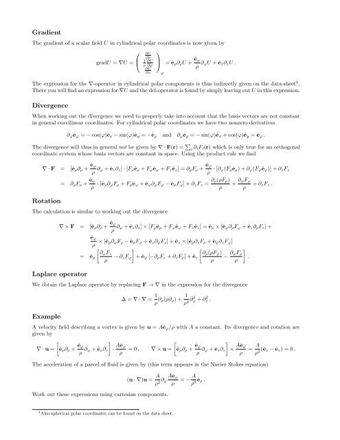
Gradient The gradient of a scalar field U in cylindrical polar coordinates is now given by ⎛ gradU = ∇U = ⎝ ∂U ∂ρ 1 ∂U ρ ∂ϕ ∂U ∂z ⎞ ⎠ p = ê ρ ∂ ρ U + êϕ ρ ∂ ϕU + ê z ∂ z U . The expression for the ∇-operator in cylindrical polar components is thus indirectly given on the data-sheet 3 . There you will find an expression for ∇U and the del-operator is found by simply leaving out U in this expression. Divergence When working out the divergence we need to properly take into account that the basis vectors are not constant in general curvilinear coordinates. For cylindrical polar coordinates we have two nonzero derivatives ∂ ϕ ê ϕ = − cos(ϕ)ê x − sin(ϕ)ê y = −ê ρ and ∂ ϕ ê ρ = − sin(ϕ)ê x + cos(ϕ)ê y = ê ϕ . The divergence will thus in general not be given by ∇ · F(r) = ∑ i ∂ iF i (r) which is only true for an orthogonal coordinate system whose basis vectors are constant in space. Using the product rule we find ∇ · F = [ê ρ ∂ ρ + êϕ ρ ∂ ϕ + ê z ∂ z ] · [F ρ ê ρ + F ϕ ê ϕ + F z ê z ] = ∂ ρ F ρ + êϕ ρ · [∂ ϕ(F ρ ê ρ ) + ∂ ϕ (F ϕ ê ϕ )] + ∂ z F z Rotation = ∂ ρ F ρ + êϕ ρ · [ê ρ∂ ϕ F ρ + F ρ ê ϕ + ê ϕ ∂ ϕ F ϕ − ê ρ F ϕ ] + ∂ z F z = ∂ ρ(ρF ρ ) + ∂ ϕF ϕ + ∂ z F z . ρ ρ The calculation is similar to working out the divergence ∇ × F = [ê ρ ∂ ρ + êϕ ρ ∂ ϕ + ê z ∂ z ] × [F ρ ê ρ + F ϕ ê ϕ + F z ê z ] = ê ρ × [ê ϕ ∂ ρ F ϕ + ê z ∂ ρ F z ] + ê ϕ ρ × [ê ρ∂ ϕ F ρ − ê ρ F ϕ + ê z ∂ ϕ F z ] + ê z × [ê ρ ∂ z F ρ + ê ϕ ∂ z F ϕ ] = ê ρ [ ∂ϕ F z ρ ] [ ∂ρ (ρF ϕ ) − ∂ z F ϕ + ê ϕ [−∂ ρ F z + ∂ z F ρ ] + ê z − ∂ ] ϕF ρ . ρ ρ Laplace operator We obtain the Laplace operator by replacing F → ∇ in the expression for the divergence ∆ = ∇ · ∇ = 1 ρ ∂ ρ(ρ∂ ρ ) + 1 ρ 2 ∂2 ϕ + ∂ 2 z . Example A velocity field describing a vortex is given by u = Aê ϕ /ρ with A a constant. Its divergence and rotation are given by [ ] ∇ · u = ê ρ ∂ ρ + êϕ ρ ∂ ϕ + ê z ∂ z · Aê [ ] ϕ = 0 , ∇ × u = ê ρ ∂ ρ + êϕ ρ ρ ∂ ϕ + ê z ∂ z × Aê ϕ = A ρ ρ 2 (ê z − ê z ) = 0 . The acceleration of a parcel of fluid is given by (this term appears in the Navier Stokes equation) (u · ∇)u = A ρ 2 ∂ Aê ϕ ϕ = − A ρ ρ 3 êρ . Work out these expressions using cartesian components. 3 Also spherical polar coordinates can be found on the data sheet.
Page 1: Vector calculus in curvilinear coor

Vector calculus in curvilinear coordinates Goals: Coordinate ...

Create successful ePaper yourself

Delete template?

Save as template?