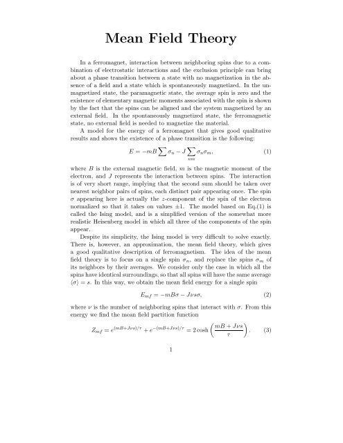
Notes on Mean Field Theory
Notes on Mean Field Theory
Notes on Mean Field Theory

You also want an ePaper? Increase the reach of your titles
YUMPU automatically turns print PDFs into web optimized ePapers that Google loves.
<strong>Mean</strong> <strong>Field</strong> <strong>Theory</strong><br />
In a ferromagnet, interacti<strong>on</strong> between neighboring spins due to a combinati<strong>on</strong><br />
of electrostatic interacti<strong>on</strong>s and the exclusi<strong>on</strong> principle can bring<br />
about a phase transiti<strong>on</strong> between a state with no magnetizati<strong>on</strong> in the absence<br />
of a field and a state which is sp<strong>on</strong>taneously magnetized. In the unmagnetized<br />
state, the paramagnetic state, the average spin is zero and the<br />
existence of elementary magnetic moments associated with the spin is shown<br />
by the fact that the spins can be aligned and the system magnetized by an<br />
external field. In the sp<strong>on</strong>taneously magnetized state, the ferromagnetic<br />
state, no external field is needed to magnetize the material.<br />
A model for the energy of a ferromagnet that gives good qualitative<br />
results and shows the existence of a phase transiti<strong>on</strong> is the following:<br />
E = −mB ∑ σ n − J ∑ nm<br />
σ n σ m , (1)<br />
where B is the external magnetic field, m is the magnetic moment of the<br />
electr<strong>on</strong>, and J represents the interacti<strong>on</strong> between spins. The interacti<strong>on</strong><br />
is of very short range, implying that the sec<strong>on</strong>d sum should be taken over<br />
nearest neighbor pairs of spins, each distinct pair appearing <strong>on</strong>ce. The spin<br />
σ appearing here is actually the z-comp<strong>on</strong>ent of the spin of the electr<strong>on</strong><br />
normalized so that it takes <strong>on</strong> values ±1. The model based <strong>on</strong> Eq.(1) is<br />
called the Ising model, and is a simplified versi<strong>on</strong> of the somewhat more<br />
realistic Heisenberg model in which all three of the comp<strong>on</strong>ents of the spin<br />
appear.<br />
Despite its simplicity, the Ising model is very difficult to solve exactly.<br />
There is, however, an approximati<strong>on</strong>, the mean field theory, which gives<br />
a good qualitative descripti<strong>on</strong> of ferromagnetism. The idea of the mean<br />
field theory is to focus <strong>on</strong> a single spin σ n , and replace the spins σ m of<br />
its neighbors by their averages. We c<strong>on</strong>sider <strong>on</strong>ly the case in which all the<br />
spins have identical surroundings, so that all spins will have the same average<br />
〈σ〉 = s. In this way, we obtain the mean field energy for a single spin<br />
E mf = −mBσ − Jνsσ, (2)<br />
where ν is the number of neighboring spins that interact with σ. From this<br />
energy we find the mean field partiti<strong>on</strong> functi<strong>on</strong><br />
( )<br />
mB + Jνs<br />
Z mf = e (mB+Jνs)/τ + e −(mB+Jνs)/τ = 2 cosh<br />
. (3)<br />
τ<br />
1
Recalling that the first term is the relative probability of σ = +1 and the<br />
sec<strong>on</strong>d is the relative probability of σ = −1, we easily find the average spin<br />
to be<br />
( )<br />
mB + Jνs<br />
s = tanh<br />
. (4)<br />
τ<br />
This equality is a self-c<strong>on</strong>sistency c<strong>on</strong>diti<strong>on</strong> for the average spin s.<br />
Figure 1:<br />
Soluti<strong>on</strong>s of the mean field equati<strong>on</strong> for (i) τ > Jν, and (ii)τ < Jν.<br />
C<strong>on</strong>sider this c<strong>on</strong>diti<strong>on</strong> in the absence of an external field. The equati<strong>on</strong><br />
s = tanh Jνs/τ can be solved graphically by plotting the left hand side and<br />
the right hand side <strong>on</strong> the same graph as functi<strong>on</strong>s of s. Where the plots<br />
intersect, there is a soluti<strong>on</strong>. There are two possibilities: (i) if Jν/τ < 1,<br />
there is there is a single soluti<strong>on</strong> s = 0, and (ii) if Jν/τ > 1, there are three<br />
soluti<strong>on</strong>s, s = 0, ±s 1 (τ). See Figure (). Since the two states with n<strong>on</strong>-zero s<br />
have the same free energy, they are the stable states because the state with<br />
s = 0 has a higher free energy. The mean field free energy can be calculated<br />
from the standard equati<strong>on</strong> F = −τ log Z, giving<br />
F mf = −Nτ log(2 cosh Jν/τ) (5)<br />
if there a total of N spins. Thus the theory predicts that at high temperature<br />
τ > Jν, the average spin, and hence the total magnetizati<strong>on</strong> M = Nms, is<br />
2
zero, while at low temperature τ < Jν there is a magnetizati<strong>on</strong> of magnitude<br />
Nms 1 (τ), which can be in either directi<strong>on</strong>. The transiti<strong>on</strong> takes place at a<br />
critical temperature τ c = Jν. This is the paramagnetic-ferromagnetic phase<br />
transiti<strong>on</strong>.<br />
Magnetizati<strong>on</strong> near τ c . We can find the magnetizati<strong>on</strong> as a functi<strong>on</strong><br />
of the temperature near the critical temperature from the self c<strong>on</strong>sistency<br />
equati<strong>on</strong>, which can be written s = tanh(τ c s/τ), by expanding the hyperbolic<br />
tangent to third order in s. The resulting equati<strong>on</strong> is<br />
τ 3 c<br />
s = τ c<br />
τ s − 1 3 τ 3 s3 . (6)<br />
Solving this for s, we obtain the magnetizati<strong>on</strong><br />
√<br />
M = Nms ≈ Nm 3 τ c − τ<br />
, (7)<br />
τ c<br />
correct to first order in the temperature difference τ c − τ. Thus the magnetizati<strong>on</strong><br />
increases very rapidly below the critical temperature, having a<br />
behavior something like the <strong>on</strong>e shown in Figure ().<br />
Figure 2:<br />
Magnetizati<strong>on</strong> as a functi<strong>on</strong> of temperature<br />
Susceptibility above τ c . Just above the critical temperature, there is<br />
no sp<strong>on</strong>taneous magnetizati<strong>on</strong>, but we can see the effect of an external field<br />
3
y expanding the full equati<strong>on</strong> s = tanh(mB + Jνs)/τ assuming that both<br />
s and B are small. The result is<br />
M = Nms = Nm2<br />
τ − τ c<br />
B (8)<br />
The coefficient of B is a quantity called the magnetic susceptibility. Its<br />
divergence at the critical temperature is a sign that the system is <strong>on</strong> the<br />
verge of being ordered: a very small magnetic field will produce a large<br />
magnetizati<strong>on</strong>.<br />
Energy and heat capacity. The energy U of the system is best obtained<br />
directly from Eq. (1), since the standard method of obtaining it from<br />
Z mf would overcount the interacti<strong>on</strong> terms. If the number of spins is N,<br />
the number of nearest neighbor pairs is Nν/2. Therefore, Eq. (1) gives<br />
The heat capacity is<br />
U = −NmBs − 1 2 NνJs 2 . (9)<br />
C = ∂U<br />
∂τ<br />
= −NmB<br />
ds<br />
dτ −1 2 NνJ ds2<br />
dτ . (10)<br />
Since the derivatives of s and s 2 with respect to τ are both negative, as<br />
indicated in Figure (), the heat capacity is positive. When the external field<br />
B is absent, C is zero above the critical temperature where s = 0. Eq. (10)<br />
shows that C is disc<strong>on</strong>tinuous at τ c , since ds/dτ is negative and finite at<br />
this point (see Eq. (7). The disc<strong>on</strong>tinuity of C at the critical temperature is<br />
characteristic of this type of phase transiti<strong>on</strong> and shows that the two phases<br />
have different physical properties.<br />
4