Notes on Mean Field Theory
Notes on Mean Field Theory
Notes on Mean Field Theory

Create successful ePaper yourself
Turn your PDF publications into a flip-book with our unique Google optimized e-Paper software.
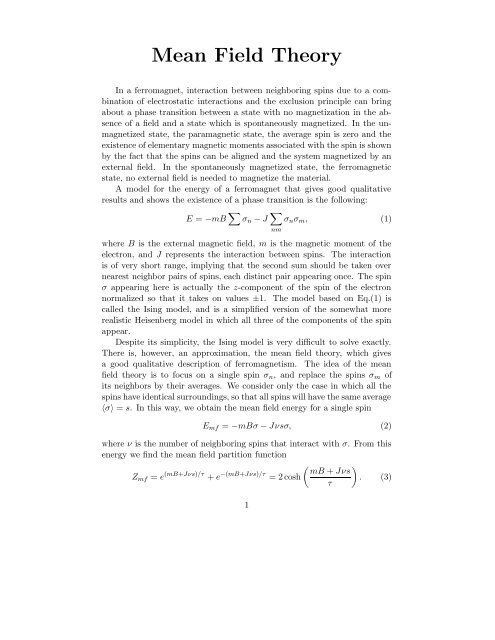
<strong>Mean</strong> <strong>Field</strong> <strong>Theory</strong><br />
In a ferromagnet, interacti<strong>on</strong> between neighboring spins due to a combinati<strong>on</strong><br />
of electrostatic interacti<strong>on</strong>s and the exclusi<strong>on</strong> principle can bring<br />
about a phase transiti<strong>on</strong> between a state with no magnetizati<strong>on</strong> in the absence<br />
of a field and a state which is sp<strong>on</strong>taneously magnetized. In the unmagnetized<br />
state, the paramagnetic state, the average spin is zero and the<br />
existence of elementary magnetic moments associated with the spin is shown<br />
by the fact that the spins can be aligned and the system magnetized by an<br />
external field. In the sp<strong>on</strong>taneously magnetized state, the ferromagnetic<br />
state, no external field is needed to magnetize the material.<br />
A model for the energy of a ferromagnet that gives good qualitative<br />
results and shows the existence of a phase transiti<strong>on</strong> is the following:<br />
E = −mB ∑ σ n − J ∑ nm<br />
σ n σ m , (1)<br />
where B is the external magnetic field, m is the magnetic moment of the<br />
electr<strong>on</strong>, and J represents the interacti<strong>on</strong> between spins. The interacti<strong>on</strong><br />
is of very short range, implying that the sec<strong>on</strong>d sum should be taken over<br />
nearest neighbor pairs of spins, each distinct pair appearing <strong>on</strong>ce. The spin<br />
σ appearing here is actually the z-comp<strong>on</strong>ent of the spin of the electr<strong>on</strong><br />
normalized so that it takes <strong>on</strong> values ±1. The model based <strong>on</strong> Eq.(1) is<br />
called the Ising model, and is a simplified versi<strong>on</strong> of the somewhat more<br />
realistic Heisenberg model in which all three of the comp<strong>on</strong>ents of the spin<br />
appear.<br />
Despite its simplicity, the Ising model is very difficult to solve exactly.<br />
There is, however, an approximati<strong>on</strong>, the mean field theory, which gives<br />
a good qualitative descripti<strong>on</strong> of ferromagnetism. The idea of the mean<br />
field theory is to focus <strong>on</strong> a single spin σ n , and replace the spins σ m of<br />
its neighbors by their averages. We c<strong>on</strong>sider <strong>on</strong>ly the case in which all the<br />
spins have identical surroundings, so that all spins will have the same average<br />
〈σ〉 = s. In this way, we obtain the mean field energy for a single spin<br />
E mf = −mBσ − Jνsσ, (2)<br />
where ν is the number of neighboring spins that interact with σ. From this<br />
energy we find the mean field partiti<strong>on</strong> functi<strong>on</strong><br />
( )<br />
mB + Jνs<br />
Z mf = e (mB+Jνs)/τ + e −(mB+Jνs)/τ = 2 cosh<br />
. (3)<br />
τ<br />
1
Recalling that the first term is the relative probability of σ = +1 and the<br />
sec<strong>on</strong>d is the relative probability of σ = −1, we easily find the average spin<br />
to be<br />
( )<br />
mB + Jνs<br />
s = tanh<br />
. (4)<br />
τ<br />
This equality is a self-c<strong>on</strong>sistency c<strong>on</strong>diti<strong>on</strong> for the average spin s.<br />
Figure 1:<br />
Soluti<strong>on</strong>s of the mean field equati<strong>on</strong> for (i) τ > Jν, and (ii)τ < Jν.<br />
C<strong>on</strong>sider this c<strong>on</strong>diti<strong>on</strong> in the absence of an external field. The equati<strong>on</strong><br />
s = tanh Jνs/τ can be solved graphically by plotting the left hand side and<br />
the right hand side <strong>on</strong> the same graph as functi<strong>on</strong>s of s. Where the plots<br />
intersect, there is a soluti<strong>on</strong>. There are two possibilities: (i) if Jν/τ < 1,<br />
there is there is a single soluti<strong>on</strong> s = 0, and (ii) if Jν/τ > 1, there are three<br />
soluti<strong>on</strong>s, s = 0, ±s 1 (τ). See Figure (). Since the two states with n<strong>on</strong>-zero s<br />
have the same free energy, they are the stable states because the state with<br />
s = 0 has a higher free energy. The mean field free energy can be calculated<br />
from the standard equati<strong>on</strong> F = −τ log Z, giving<br />
F mf = −Nτ log(2 cosh Jν/τ) (5)<br />
if there a total of N spins. Thus the theory predicts that at high temperature<br />
τ > Jν, the average spin, and hence the total magnetizati<strong>on</strong> M = Nms, is<br />
2
zero, while at low temperature τ < Jν there is a magnetizati<strong>on</strong> of magnitude<br />
Nms 1 (τ), which can be in either directi<strong>on</strong>. The transiti<strong>on</strong> takes place at a<br />
critical temperature τ c = Jν. This is the paramagnetic-ferromagnetic phase<br />
transiti<strong>on</strong>.<br />
Magnetizati<strong>on</strong> near τ c . We can find the magnetizati<strong>on</strong> as a functi<strong>on</strong><br />
of the temperature near the critical temperature from the self c<strong>on</strong>sistency<br />
equati<strong>on</strong>, which can be written s = tanh(τ c s/τ), by expanding the hyperbolic<br />
tangent to third order in s. The resulting equati<strong>on</strong> is<br />
τ 3 c<br />
s = τ c<br />
τ s − 1 3 τ 3 s3 . (6)<br />
Solving this for s, we obtain the magnetizati<strong>on</strong><br />
√<br />
M = Nms ≈ Nm 3 τ c − τ<br />
, (7)<br />
τ c<br />
correct to first order in the temperature difference τ c − τ. Thus the magnetizati<strong>on</strong><br />
increases very rapidly below the critical temperature, having a<br />
behavior something like the <strong>on</strong>e shown in Figure ().<br />
Figure 2:<br />
Magnetizati<strong>on</strong> as a functi<strong>on</strong> of temperature<br />
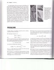
Susceptibility above τ c . Just above the critical temperature, there is<br />
no sp<strong>on</strong>taneous magnetizati<strong>on</strong>, but we can see the effect of an external field<br />
3
y expanding the full equati<strong>on</strong> s = tanh(mB + Jνs)/τ assuming that both<br />
s and B are small. The result is<br />
M = Nms = Nm2<br />
τ − τ c<br />
B (8)<br />
The coefficient of B is a quantity called the magnetic susceptibility. Its<br />
divergence at the critical temperature is a sign that the system is <strong>on</strong> the<br />
verge of being ordered: a very small magnetic field will produce a large<br />
magnetizati<strong>on</strong>.<br />
Energy and heat capacity. The energy U of the system is best obtained<br />
directly from Eq. (1), since the standard method of obtaining it from<br />
Z mf would overcount the interacti<strong>on</strong> terms. If the number of spins is N,<br />
the number of nearest neighbor pairs is Nν/2. Therefore, Eq. (1) gives<br />
The heat capacity is<br />
U = −NmBs − 1 2 NνJs 2 . (9)<br />
C = ∂U<br />
∂τ<br />
= −NmB<br />
ds<br />
dτ −1 2 NνJ ds2<br />
dτ . (10)<br />
Since the derivatives of s and s 2 with respect to τ are both negative, as<br />
indicated in Figure (), the heat capacity is positive. When the external field<br />
B is absent, C is zero above the critical temperature where s = 0. Eq. (10)<br />
shows that C is disc<strong>on</strong>tinuous at τ c , since ds/dτ is negative and finite at<br />
this point (see Eq. (7). The disc<strong>on</strong>tinuity of C at the critical temperature is<br />
characteristic of this type of phase transiti<strong>on</strong> and shows that the two phases<br />
have different physical properties.<br />
4