Atmospheric carbon dioxide levels for the last 500 million years
Atmospheric carbon dioxide levels for the last 500 million years
Atmospheric carbon dioxide levels for the last 500 million years

Create successful ePaper yourself
Turn your PDF publications into a flip-book with our unique Google optimized e-Paper software.
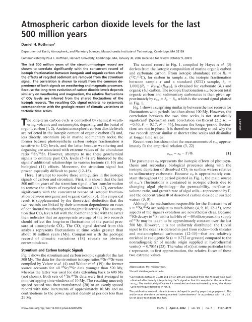
<strong>Atmospheric</strong> <strong>carbon</strong> <strong>dioxide</strong> <strong>levels</strong> <strong>for</strong> <strong>the</strong> <strong>last</strong><br />
<strong>500</strong> <strong>million</strong> <strong>years</strong><br />
Daniel H. Rothman †<br />
Department of Earth, <strong>Atmospheric</strong>, and Planetary Sciences, Massachusetts Institute of Technology, Cambridge, MA 02139<br />
Communicated by Paul F. Hoffman, Harvard University, Cambridge, MA, January 30, 2002 (received <strong>for</strong> review October 9, 2001)<br />
The <strong>last</strong> <strong>500</strong> <strong>million</strong> <strong>years</strong> of <strong>the</strong> strontium-isotope record are<br />
shown to correlate significantly with <strong>the</strong> concurrent record of<br />
isotopic fractionation between inorganic and organic <strong>carbon</strong> after<br />
<strong>the</strong> effects of recycled sediment are removed from <strong>the</strong> strontium<br />
signal. The correlation is shown to result from <strong>the</strong> common dependence<br />
of both signals on wea<strong>the</strong>ring and magmatic processes.<br />
Because <strong>the</strong> long-term evolution of <strong>carbon</strong> <strong>dioxide</strong> <strong>levels</strong> depends<br />
similarly on wea<strong>the</strong>ring and magmatism, <strong>the</strong> relative fluctuations<br />
of CO 2 <strong>levels</strong> are inferred from <strong>the</strong> shared fluctuations of <strong>the</strong><br />
isotopic records. The resulting CO 2 signal exhibits no systematic<br />
correspondence with <strong>the</strong> geologic record of climatic variations at<br />
tectonic time scales.<br />
The long-term <strong>carbon</strong> cycle is controlled by chemical wea<strong>the</strong>ring,<br />
volcanic and metamorphic degassing, and <strong>the</strong> burial of<br />
organic <strong>carbon</strong> (1, 2). Ancient atmospheric <strong>carbon</strong> <strong>dioxide</strong> <strong>levels</strong><br />
are reflected in <strong>the</strong> isotopic content of organic <strong>carbon</strong> (3) and,<br />
less directly, strontium (4) in marine sedimentary rocks; <strong>the</strong><br />
<strong>for</strong>mer because photosyn<strong>the</strong>tic <strong>carbon</strong> isotope fractionation is<br />
sensitive to CO 2 <strong>levels</strong>, and <strong>the</strong> latter because wea<strong>the</strong>ring and<br />
degassing are associated with extreme values of <strong>the</strong> abundance<br />
ratio 87 Sr 86 Sr. However, attempts to use <strong>the</strong>se geochemical<br />
signals to estimate past CO 2 <strong>levels</strong> (5–8) are hindered by <strong>the</strong><br />
signals’ additional relationships to various tectonic (9, 10) and<br />
biological (11) effects. Moreover, <strong>the</strong> strontium signal has<br />
proven especially difficult to parse (12–15).<br />
Here, I attempt to resolve <strong>the</strong>se ambiguities in <strong>the</strong> isotopic<br />
signals of <strong>carbon</strong> and strontium. First, it is shown that <strong>the</strong> <strong>last</strong><br />
<strong>500</strong> <strong>million</strong> <strong>years</strong> of <strong>the</strong> strontium signal, after trans<strong>for</strong>mation<br />
to remove <strong>the</strong> effects of recycled sediment (16, 17), correlate<br />
significantly with <strong>the</strong> concurrent record of isotopic fractionation<br />
between inorganic and organic <strong>carbon</strong> (3). This empirical<br />
result is supplemented by <strong>the</strong> <strong>the</strong>oretical deduction that <strong>the</strong><br />
two records are linked by <strong>the</strong>ir common dependence on rates<br />
of continental wea<strong>the</strong>ring and magmatic activity. The assumption<br />
that CO 2 <strong>levels</strong> fall with <strong>the</strong> <strong>for</strong>mer and rise with <strong>the</strong> latter<br />
<strong>the</strong>n indicates that an appropriate average of <strong>the</strong> two records<br />
should reflect <strong>the</strong> long-term fluctuations of <strong>the</strong> partial pressure<br />
of atmospheric CO 2 . The CO 2 signal derived from this<br />
analysis represents fluctuations at time scales greater than<br />
about 10 <strong>million</strong> <strong>years</strong> (My). Comparison with <strong>the</strong> geologic<br />
record of climatic variations (18) reveals no obvious<br />
correspondence.<br />
Strontium and Carbon Isotopic Signals<br />
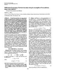
Fig. 1 shows <strong>the</strong> strontium and <strong>carbon</strong> isotopic signals <strong>for</strong> <strong>the</strong> <strong>last</strong><br />
<strong>500</strong> My. The data <strong>for</strong> <strong>the</strong> strontium isotope ratios 87 Sr 86 Sr were<br />
compiled by Veizer et al. (4) and Walter et al. (19); <strong>the</strong> <strong>for</strong>mer<br />
source accounts <strong>for</strong> all 87 Sr 86 Sr data younger than 520 My,<br />
whereas <strong>the</strong> latter was used <strong>for</strong> data extending back to 608 My<br />
(not shown). Both sets of 87 Sr 86 Sr data were first averaged in<br />
nonoverlapping time windows of 10 My. The resulting unevenly<br />
spaced record was <strong>the</strong>n trans<strong>for</strong>med (20) to an evenly spaced<br />
record with time increments of approximately 10 My and no<br />
contributions to <strong>the</strong> power spectral density at periods less than<br />
21 My.<br />
The second record in Fig. 1, compiled by Hayes et al. (3)<br />
derives from <strong>the</strong> isotopic composition of marine organic <strong>carbon</strong><br />
and <strong>carbon</strong>ate <strong>carbon</strong>. From isotopic abundance ratios R x <br />
( 13 C 12 C) x <strong>for</strong> <strong>carbon</strong> in sample x, <strong>the</strong> isotopic fractionation<br />
between sample x and a standard (STD) sample, x <br />
1,000[(R x R STD )R STD ], is obtained <strong>for</strong> <strong>carbon</strong>ate ( a ) and<br />
organic ( o ) <strong>carbon</strong>. The isotopic fractionation toc between total<br />
organic <strong>carbon</strong> and sedimentary <strong>carbon</strong>ates is <strong>the</strong>n given approximately<br />
by toc a o , which is <strong>the</strong> second signal plotted<br />
in Fig. 1.<br />
Fig. 1 shows a surprising similarity between <strong>the</strong> two records <strong>for</strong><br />
fluctuations with periods less than about 100 My. However, <strong>the</strong><br />
correlation between <strong>the</strong> two time series is not statistically<br />
significant ‡ [Spearman rank correlation coefficient (21) R s <br />
0.40, P 0.17, N 46], because <strong>the</strong> longer-period fluctuations<br />
are not in phase. It is <strong>the</strong>re<strong>for</strong>e interesting to ask why <strong>the</strong><br />
two records appear similar at shorter time scales and dissimilar<br />
at longer time scales.<br />
Recent work has shown that <strong>the</strong> measurements of toc approximately<br />
fit <strong>the</strong> empirical relation (3, 22)<br />
toc 0 . [1]<br />
The parameter 0 represents <strong>the</strong> isotopic effects of photosyn<strong>the</strong>sis<br />
and secondary biological processes along with <strong>the</strong><br />
isotopic depletion of dissolved CO 2 in surface waters relative<br />
to sedimentary <strong>carbon</strong>ate. Because 0 is approximately constant<br />
throughout <strong>the</strong> period plotted in Fig. 1, <strong>the</strong> main source<br />
of toc ’s fluctuations is contained in isotopic effects due to<br />
changing algal physiology—<strong>the</strong> permeability, surface-tovolume<br />
ratio, and growth rate of algal cells—represented by ,<br />
and <strong>the</strong> concentration of dissolved <strong>carbon</strong> <strong>dioxide</strong> in surface<br />
waters (3, 8).<br />
Although <strong>the</strong> mechanisms responsible <strong>for</strong> <strong>the</strong> fluctuations of<br />
s 87 Sr 86 Sr are subject to much debate (4, 9, 10, 12–15), some<br />
aspects of <strong>the</strong> signal’s evolution are never<strong>the</strong>less clear. Because<br />
87 Rb decays to 87 Sr with a half-life of 48 billion <strong>years</strong>, <strong>the</strong> supply<br />
of 87 Sr may be taken to be approximately constant over <strong>the</strong> <strong>last</strong><br />
<strong>500</strong> My. However, it is not uni<strong>for</strong>mly distributed: <strong>the</strong> fluvial<br />
input to <strong>the</strong> oceans is derived in part from rocks—both silicates<br />
and metamorphosed <strong>carbon</strong>ates (12–15)—that are relatively<br />
enriched in radiogenic Sr (s 0.712 or greater) compared to <strong>the</strong><br />
nonradiogenic Sr of mantle origin supplied at hydro<strong>the</strong>rmal<br />
vents (s 0.7035) (23). The value of s(t) at some particular time<br />
t represents, to first approximation, <strong>the</strong> relative fluxes of <strong>the</strong>se<br />
two extreme values.<br />
Abbreviation: My, <strong>million</strong> <strong>years</strong>.<br />
† E-mail: dan@segovia.mit.edu.<br />
‡ Correlations between toc(t) and s(t) org(t) are computed from <strong>the</strong> N equal-time pairs<br />
obtained after linearly interpolating <strong>the</strong> Sr signal so that it is sampled at <strong>the</strong> same times<br />
as toc. The statistical significance P is one-sided and was estimated by using <strong>the</strong> Monte<br />
Carlo technique described in ref. 8.<br />
The publication costs of this article were defrayed in part by page charge payment. This<br />
article must <strong>the</strong>re<strong>for</strong>e be hereby marked “advertisement” in accordance with 18 U.S.C.<br />
§1734 solely to indicate this fact.<br />
GEOLOGY<br />
www.pnas.orgcgidoi10.1073pnas.022055499 PNAS April 2, 2002 vol. 99 no. 7 4167–4171
volcanic degassing. Assuming that r r(w) and v h v h (v), g’s<br />
dependence on w and v may be written § drdw 0, dudw 0, and dv h dv 0. [7]<br />
g grw, v h v. [4]<br />
With respect to toc , <strong>the</strong> physiological term may likewise<br />
depend on w because of changing nutrient concentrations in <strong>the</strong><br />
oceans. could also depend on CO 2 <strong>levels</strong>, which in turn depend<br />
on degassing, wea<strong>the</strong>ring rates—because of <strong>the</strong> net uptake rate<br />
u u(w) of atmospheric CO 2 associated with silicate wea<strong>the</strong>ring<br />
(1, 2, 24)—and o<strong>the</strong>r processes, such as organic <strong>carbon</strong> burial,<br />
which we collectively designate by b. Aggregating <strong>the</strong>se dependencies<br />
<strong>the</strong>n yields<br />
w, uw, v, b<br />
toc 0 .<br />
uw, v, b<br />
[5]<br />
Comparison of Eqs. 4 and 5 directly reveals <strong>the</strong> joint dependence<br />
of g and toc on v and w.<br />
Removal of <strong>the</strong> Effects of Sedimentary Recycling<br />
Fig. 1. Data <strong>for</strong> toc (red filled circles) (3) and 87 Sr 86 Sr (blue open squares) (4). Because <strong>the</strong> strontium signal s contains a memory effect,<br />
The time scale <strong>for</strong> toc has been revised from <strong>the</strong> original to match <strong>the</strong> scheme whereas toc does not, removal of <strong>the</strong> memory effect should<br />
(32) used <strong>for</strong> <strong>the</strong> strontium data. The capital letters correspond to <strong>the</strong> following<br />
geologic periods: Ordovician, Silurian, Devonian, Carboniferous, Permian,<br />
Triassic, Jurassic, Cretaceous, and Tertiary.<br />
reveal correlations between s and toc at both short and long time<br />
scales, <strong>the</strong>reby confirming <strong>the</strong> joint dependence on v and w. To<br />
test this hypo<strong>the</strong>sis, I first assume it is true and use it to estimate<br />
g. For a given and , m is calculated by discretizing Eq. 3 <strong>for</strong><br />
However, this first approximation ignores <strong>the</strong> recycling of<br />
rocks in <strong>the</strong> sedimentary cycle (16). As pointed out by Brass (17),<br />
about 75% of <strong>the</strong> strontium input to <strong>the</strong> oceans should come<br />
from <strong>the</strong> wea<strong>the</strong>ring of exposed <strong>carbon</strong>ates of marine origin.<br />
608 My. Eq. 2 is <strong>the</strong>n solved <strong>for</strong> g:<br />
g s m <br />
1 . [6]<br />
Because <strong>the</strong>se <strong>carbon</strong>ates retain a memory of s at <strong>the</strong> time of Here <strong>the</strong> subscripts make explicit <strong>the</strong> dependencies on and .<br />
deposition, <strong>the</strong>ir contribution to sedimentary Sr significantly Let R ( toc , g ) be <strong>the</strong> Pearson product-moment correlation<br />
damps <strong>the</strong> signal coming from hydro<strong>the</strong>rmal vents (low s) and<br />
rocks containing radiogenic Sr (high s) (9).<br />
coefficient (21) that quantifies <strong>the</strong> similarity of toc and g .<br />
From <strong>the</strong> <strong>for</strong>egoing argument, <strong>the</strong> best estimate of and <br />
Denoting <strong>the</strong> fluvial flux of radiogenic Sr by r, <strong>the</strong> input from should be that which minimizes R (because <strong>the</strong> expected<br />
hydro<strong>the</strong>rmal vents by v h , and <strong>the</strong> memory effect by m, a simple<br />
expression <strong>for</strong> <strong>the</strong> strontium isotope ratio s is<br />
correlation is negative). Fig. 2 shows contours of R as a function<br />
of and t1 2<br />
(ln 2). The minimum R 0.81 occurs at<br />
s m 1 gr, v h , [2]<br />
t1 2<br />
54 My and 0.99. However, <strong>the</strong> corresponding estimate<br />
of g includes values below <strong>the</strong> hydro<strong>the</strong>rmal minimum of<br />
0.7035. Such nonphysical ratios probably derive from <strong>the</strong> amplification<br />
of any measurement noise resulting from division by<br />
where 0 1 is <strong>the</strong> fraction of sedimentary Sr deriving from<br />
<strong>the</strong> memory flux, and g is a function that depends on both r and <strong>the</strong> small quantity 1 in Eq. 6. Indeed, <strong>the</strong> dark gray region<br />
v h . The memory term can be approximated by assuming that in Fig. 2 indicates that all such results occur only <strong>for</strong> close to<br />
sedimentary strontium is wea<strong>the</strong>red at a rate proportional to its unity. I <strong>the</strong>re<strong>for</strong>e define <strong>the</strong> best estimates *, * of, by<br />
mass (16). Then m(t) is simply a weighted (exponentially decaying)<br />
average of s(), t (17), which we express by <strong>the</strong> <strong>the</strong>n finds<br />
minimizing R subject to <strong>the</strong> constraint that g 0.7035. One<br />
convolution<br />
2<br />
ln 2* 41 My and * 0.83, corresponding<br />
to R ** 0.80 (within 1% of <strong>the</strong> unconstrained minimum).<br />
These results are in reasonable accord with Brass’s estimate of<br />
t<br />
<strong>the</strong> half-life of sedimentary Sr (57 102 My) (17) and his<br />
mt e <br />
sd. [3] conclusion that ‘‘strontium leached from limestones is about<br />
75% of <strong>the</strong> total input’’ (17).<br />
Fig. 3 shows g ** compared to toc . Compared with Fig. 1, one<br />
The parameter is related to <strong>the</strong> half-life t1 2<br />
of sedimentary Sr;<br />
sees that both <strong>the</strong> long and short period fluctuations are now not<br />
i.e., (ln 2)t1 2<br />
. Brass estimates 57 My t1 2<br />
102 My (17). only approximately equally correlated, but <strong>the</strong> correlation is also<br />
There<strong>for</strong>e, <strong>the</strong> memory effect should strongly influence <strong>the</strong> significant (R s 0.74, P 10 3 , N 46). The hypo<strong>the</strong>sis that<br />
fluctuations of s at long time scales (greater than about 100 My), recycled sediment partially obscured an inherent correlation<br />
whereas <strong>the</strong> short time scale fluctuations should be relatively because of a shared dependence on wea<strong>the</strong>ring and volcanic<br />
unaffected.<br />
processes is <strong>the</strong>re<strong>for</strong>e confirmed.<br />
The short-time correlations may be explained in part by noting<br />
<strong>the</strong> common dependence of toc and g on <strong>the</strong> global wea<strong>the</strong>ring<br />
rate w (i.e., <strong>the</strong> flux of all wea<strong>the</strong>red products from <strong>the</strong> continents<br />
to <strong>the</strong> oceans) and <strong>the</strong> rate of magmatic activity v<br />
associated not only with <strong>the</strong> hydro<strong>the</strong>rmal flux v h but also with<br />
Relationship to CO 2 Levels<br />
To understand fur<strong>the</strong>r <strong>the</strong> correlation, I make <strong>the</strong> following<br />
assumptions concerning <strong>the</strong> functional dependencies contained<br />
in Eqs. 4 and 5:<br />
§ Although w and v could conceivably depend on one ano<strong>the</strong>r, here such dependencies are<br />
assumed to be insignificant compared to any independent variations.<br />
The first two state that <strong>the</strong> flux of radiogenic Sr to <strong>the</strong> oceans<br />
and <strong>the</strong> uptake of atmospheric CO 2 because of silicate wea<strong>the</strong>ring<br />
increase as <strong>the</strong> global wea<strong>the</strong>ring rate (of all minerals in all<br />
4168 www.pnas.orgcgidoi10.1073pnas.022055499 Rothman
Fig. 3. The function g (blue squares) obtained by removing <strong>the</strong> memory flux<br />
from <strong>the</strong> 87 Sr 86 Sr data of Fig. 1, along with toc (red circles). Note that <strong>the</strong><br />
range of <strong>the</strong> 87 Sr 86 Sr curve is approximately five times greater than in Fig. 1.<br />
The data are plotted such that <strong>the</strong> mean of both time series lies on <strong>the</strong> same<br />
horizontal line and <strong>the</strong>ir rms fluctuations have <strong>the</strong> same vertical extent.<br />
Thus <strong>the</strong> shared fluctuations of g and toc indicate <strong>the</strong> relative<br />
Fig. 2. Contours of R as a function of , <strong>the</strong> fraction of sedimentary Sr<br />
<br />
<br />
0 and<br />
v w du<br />
u dw 0. [10]<br />
deriving from <strong>the</strong> memory flux, and t1 2<br />
(ln 2), <strong>the</strong> half-life of sedimentary<br />
fluctuations of ancient CO 2 <strong>levels</strong>. <br />
Sr. R was calculated <strong>for</strong> 0, 0.01, ...,0.99 and t1 2 1,2,...,99My. For large half-life, <strong>the</strong> contours decrease from left to right as follow: 0.60, Estimation of <strong>the</strong> CO 2 Signal<br />
0.65, 0.70, 0.75, 0.79. The symbol marks <strong>the</strong> minimum, R ** 0.80,<br />
obtained under <strong>the</strong> constraint that g(t) 0.7035. The area shaded dark gray I proceed to estimate <strong>the</strong> CO 2 signal explicitly. First, <strong>the</strong> highest<br />
on <strong>the</strong> right does not satisfy <strong>the</strong> constraint. The rectangular area labeled measurement of toc ,at175 My, is dropped because of its<br />
‘‘Brass’’ corresponds to previous estimates obtained by geochemical arguments<br />
statistical insignificance (3). I <strong>the</strong>n trans<strong>for</strong>m g(t) 3 g (t), a<br />
(17); its horizontal extent has not been explicitly computed.<br />
strontium-derived estimate of toc , by mapping <strong>the</strong> left axis of<br />
Fig. 3 to <strong>the</strong> corresponding value on <strong>the</strong> right axis. The quantities<br />
toc and g are <strong>the</strong>n averaged to obtain<br />
terranes) increases. The third <strong>for</strong>malizes <strong>the</strong> natural assumption<br />
that <strong>the</strong> hydro<strong>the</strong>rmal flux of Sr varies with <strong>the</strong> same sign as all<br />
t i g t i toc t i 2. [11]<br />
magmatic processes.<br />
Because <strong>the</strong> Sr isotope ratios increase with increasing r (i.e.,<br />
The times t i are given by <strong>the</strong> points where toc is specified and<br />
g (t i ) is obtained by linear interpolation. Here it is implicitly<br />
gr 0) and decrease with increasing v h (i.e., gv h 0), one assumed that toc and g contain a common signal that is<br />
has<br />
enhanced by averaging. Statistical arguments suggest that ’srms<br />
signal-to-noise ratio lies between about 2 and 3.**<br />
g<br />
v g dv h<br />
v h dv 0 and g<br />
w g dr<br />
Assume now that and 0 are constant and define <strong>the</strong><br />
0. [8] dimensionless CO<br />
r dw 2 concentration 0 (8). In terms of <br />
and , Eq. 1 <strong>the</strong>n yields<br />
Because g and toc are negatively correlated, one expects that toc<br />
depends on v and w in <strong>the</strong> opposite sense:<br />
0<br />
t <br />
0 t . [12]<br />
toc v 0 and toc w 0. [9] At long time scales such that <strong>the</strong> oceans are in equilibrium with<br />
<strong>the</strong> atmosphere, <strong>the</strong> partial pressure pCO 2 is proportional to <br />
The inequalities 8 and 9 have been obtained without making any<br />
explicit assumption concerning any dependence of r on u nor <br />
(1). The relative fluctuations of pCO 2 are <strong>the</strong>re<strong>for</strong>e given by<br />
(t)(0), which is plotted in Fig. 4 <strong>for</strong> 0 36 per mil (‰).<br />
on v and w. Because <strong>the</strong>y show that v and w each influence g and<br />
toc with opposite signs, <strong>the</strong> relative fluctuations of any o<strong>the</strong>r<br />
quantity that also depends on v and w with opposite signs may<br />
Because can also depend on o<strong>the</strong>r processes b such as organic <strong>carbon</strong> burial, <strong>the</strong> shared<br />
fluctuations of g and toc do not necessarily reflect <strong>the</strong> full evolution of but ra<strong>the</strong>r <strong>the</strong><br />
be inferred from <strong>the</strong> shared fluctuations of g and toc . Specifically,<br />
<strong>the</strong> concentration of oceanic CO 2 responds positively to<br />
v while its response to wea<strong>the</strong>ring is negative:<br />
‘‘partial’’ contribution of v and w alone. However, <strong>the</strong> good correlation of Fig. 3 indicates<br />
that b’sinfluence on ’s fluctuations has been small, except possibly in <strong>the</strong> Carboniferous.<br />
Thus one may conclude that <strong>the</strong> fluctuations of g and toc follow to good approximation<br />
<strong>the</strong> fluctuations of with opposite signs.<br />
One also requires that if changes in v or w dominate one process <strong>the</strong>n <strong>the</strong>y dominate all<br />
processes.<br />
**To estimate <strong>the</strong> signal-to-noise ratio of <strong>the</strong> time series (t)defined by Eq. 11, assume that<br />
toc and g are each composed of a shared but unknown signal z in <strong>the</strong> presence of<br />
zero-mean noise toc and g, respectively: toc z toc and g z g. The quantity<br />
is an estimate of z. Its signal-to-noise ratio may be computed under <strong>the</strong> assumption that<br />
toc and g each have variance 2 , z has variance z 2 , and toc, g, and z are each<br />
uncorrelated to <strong>the</strong> o<strong>the</strong>r. The expectation of <strong>the</strong> correlation coefficient R is <strong>the</strong>n z 2 <br />
( z 2 2 ) (25). The observed correlation R 0.80 <strong>the</strong>n yields z 2 2 4, or that <strong>the</strong> rms<br />
signal fluctuation is twice that of <strong>the</strong> noise. The rms signal-to-noise ratio of can be as<br />
large as a factor of 2 greater, i.e., it should range between about 2 and 3.<br />
GEOLOGY<br />
Rothman PNAS April 2, 2002 vol. 99 no. 7 4169
4. The gray bars at <strong>the</strong> top of Fig. 4 correspond to <strong>the</strong> periods<br />
when <strong>the</strong> global climate was cool; <strong>the</strong> intervening white space<br />
corresponds to <strong>the</strong> warm modes (18). The most recent cool<br />
period corresponds to relatively low CO 2 <strong>levels</strong>, as is widely<br />
expected (30). However, no correspondence between pCO 2 and<br />
climate is evident in <strong>the</strong> remainder of <strong>the</strong> record, in part because<br />
<strong>the</strong> apparent 100 My cycle of <strong>the</strong> pCO 2 record does not match<br />
<strong>the</strong> longer climatic cycle. The lack of correlation remains if one<br />
calculates <strong>the</strong> change in average global surface temperature<br />
resulting from changes in pCO 2 and <strong>the</strong> solar constant using<br />
energy-balance arguments (7, 26).<br />
Superficially, this observation would seem to imply that pCO 2<br />
does not exert dominant control on Earth’s climate at time scales<br />
greater than about 10 My. A wealth of evidence, however,<br />
suggests that pCO 2 exerts at least some control [see Crowley and<br />
Berner (30) <strong>for</strong> a recent review]. Fig. 4 cannot by itself refute this<br />
assumption. Instead, it simply shows that <strong>the</strong> ‘‘null hypo<strong>the</strong>sis’’<br />
that pCO 2 and climate are unrelated cannot be rejected on <strong>the</strong><br />
basis of this evidence alone.<br />
Fig. 4. Fluctuations of pCO 2 <strong>for</strong> <strong>the</strong> <strong>last</strong> <strong>500</strong> My, normalized by <strong>the</strong><br />
estimate of pCO 2 obtained from <strong>the</strong> most recent value of . The solid line<br />
is obtained from Eq. 12 by using 0 36‰. The lower and upper limits of<br />
<strong>the</strong> gray area surrounding <strong>the</strong> pCO 2 curve result from 0 38 and 35‰,<br />
respectively. The gray bars at <strong>the</strong> top correspond to periods when Earth’s<br />
climate was relatively cool; <strong>the</strong> white spaces between <strong>the</strong>m correspond to<br />
warm modes (18).<br />
The gray area surrounding <strong>the</strong> pCO 2 curve in Fig. 4 brackets this<br />
result <strong>for</strong> 0 35‰ and 38‰, a range consistent with previous<br />
estimates (3).<br />
Fig. 4 reveals that CO 2 <strong>levels</strong> have mostly decreased <strong>for</strong> <strong>the</strong> <strong>last</strong><br />
175 My. Prior to that point <strong>the</strong>y appear to have fluctuated from<br />
about two to four times modern <strong>levels</strong> with a dominant period<br />
of about 100 My. The decline <strong>for</strong> <strong>the</strong> <strong>last</strong> 175 My is also present<br />
in several previous pCO 2 reconstructions (7, 8, 26, 27), and <strong>the</strong><br />
entire curve displays some similarity to a previous estimate<br />
derived from <strong>the</strong> geologic record of <strong>carbon</strong>ate <strong>for</strong>mation (26).<br />
Although <strong>the</strong> period be<strong>for</strong>e 175 My differs substantially from<br />
previous geochemical model calculations (7), an approximate<br />
error estimate lends considerable credence to <strong>the</strong> pCO 2 curve of<br />
Fig. 4. Specifically, should inherit ’s signal-to-noise ratio of<br />
2–3. This correspondence would be exact if () were linear.<br />
Because () is monotonic <strong>for</strong> <strong>the</strong> observed range of , its<br />
nonlinearity does not affect <strong>the</strong> timing of <strong>the</strong> maxima and<br />
minima of <strong>the</strong> pCO 2 curve. Thus <strong>the</strong> linear error estimate<br />
remains pertinent.<br />
Comparison with <strong>the</strong> Climate Record<br />
Using a variety of sedimentological criteria, Frakes et al. (18) have<br />
concluded that Earth’s climate has cycled several times between<br />
warm and cool modes <strong>for</strong> roughly <strong>the</strong> <strong>last</strong> 600 My. Recent work by<br />
Veizer et al. (28), based on measurements of oxygen isotopes in<br />
calcite and aragonite shells, appears to confirm <strong>the</strong> existence of<br />
<strong>the</strong>se long-period (135 My) climatic fluctuations. Changes in CO 2<br />
<strong>levels</strong> are usually assumed to be among <strong>the</strong> dominant mechanisms<br />
driving such long-term climate change (29).<br />
It is <strong>the</strong>re<strong>for</strong>e interesting to ask what, if any, correspondence<br />
exists between ancient climate and <strong>the</strong> estimate of pCO 2 in Fig.<br />
Discussion and Conclusion<br />
One of <strong>the</strong> principal contributions of this study is methodological.<br />
From observations of a weak correlation between strontium<br />
and <strong>carbon</strong> isotopic signals (Fig. 1) and <strong>the</strong>ir shared dependence<br />
on global wea<strong>the</strong>ring rates and magmatic activity, wea<strong>the</strong>ring<br />
and magmatism are deduced to be <strong>the</strong> main processes driving <strong>the</strong><br />
signals’ fluctuations. Correction <strong>for</strong> <strong>the</strong> effects of sedimentary<br />
recycling enhances <strong>the</strong> correlation (Fig. 3), indicates a strong<br />
shared signal, and streng<strong>the</strong>ns this conclusion.<br />
A second, crucial step is to note that any quantity with a similar<br />
joint dependence on wea<strong>the</strong>ring and magmatic processes may be<br />
expected to display similar fluctuations. Here attention has been<br />
focused on CO 2 <strong>levels</strong>; as <strong>for</strong> <strong>the</strong> strontium and <strong>carbon</strong> isotopic<br />
signals, CO 2 <strong>levels</strong> depend on wea<strong>the</strong>ring and magmatism with<br />
opposite signs and should <strong>the</strong>re<strong>for</strong>e fluctuate roughly in sync<br />
with <strong>the</strong> isotopic signals. Because <strong>the</strong> reasoning is general, it<br />
need not be limited to CO 2 . Among <strong>the</strong> many possible applications,<br />
<strong>the</strong> case of oceanic phosphate concentrations is particularly<br />
interesting. Phosphate concentrations should increase with<br />
wea<strong>the</strong>ring and decrease with hydro<strong>the</strong>rmal activity (31); thus<br />
<strong>the</strong> methodology in this paper may be applicable to <strong>the</strong>ir<br />
reconstruction. Moreover, because phosphorus is a limiting<br />
nutrient, oceanic productivity may be expected to covary positively<br />
with its concentration in seawater, suggesting that CO 2 <strong>levels</strong><br />
and productivity covary negatively at geologic time scales (8).<br />
Such reasoning naturally raises <strong>the</strong> issue of cause and effect.<br />
This study indicates that degassing and silicate wea<strong>the</strong>ring were<br />
<strong>the</strong> primary controls on <strong>the</strong> <strong>carbon</strong> cycle <strong>for</strong> <strong>the</strong> <strong>last</strong> <strong>500</strong> My. But<br />
<strong>the</strong> results do not <strong>the</strong>mselves indicate whe<strong>the</strong>r ei<strong>the</strong>r of <strong>the</strong>se<br />
mechanisms dominated, or whe<strong>the</strong>r wea<strong>the</strong>ring was driven by<br />
<strong>the</strong> diversification of land plants (8), continental collisions (9),<br />
or a complex combination of tectonic, biological, and geochemical<br />
processes (7). They do, however, offer a new view of <strong>the</strong><br />
long-term fluctuations of pCO 2 that will hopefully stimulate<br />
novel approaches to <strong>the</strong> study of biogeochemical cycles at<br />
evolutionary time scales.<br />
I thank O. Aharonson, L. Derry, J. Hayes, P. Hoffman, A. Knoll, L.<br />
Kump, J. Sachs, R. Summons, and <strong>the</strong> late John Edmond <strong>for</strong> helpful<br />
remarks. This work was supported in part by National Science Foundation<br />
Grant DEB-0083983.<br />
1. Walker, J. C. G. (1977) Evolution of <strong>the</strong> Atmosphere (Macmillan, New York).<br />
2. Holland, H. D. (1978) The Chemistry of <strong>the</strong> Atmosphere and Oceans (Wiley, New<br />
York).<br />
3. Hayes, J. M., Strauss, H. & Kaufman, A. J. (1999) Chem. Geol. 161, 103–125.<br />
4. Veizer, J., Ala, D., Azmy, D., Bruckschen, P., Buhl, D., Bruhn, F., Carden, G.,<br />
Diener, A., Ebneth, S., Godderis, Y., et al. (1999) Chem. Geol. 161, 59–88.<br />
5. Freeman, K. & Hayes, J. M. (1992) Global Biogeochem. Cycles 6, 185–198.<br />
6. Francois, L. M. & Walker, J. C. G. (1992) Am. J. Sci. 292, 81–135.<br />
7. Berner, R. A. (1994) Am. J. Sci. 294, 56–91.<br />
8. Rothman, D. H. (2001) Proc. Natl. Acad. Sci. USA 98, 4305–4310.<br />
9. Edmond, J. (1992) Science 258, 1594–1597.<br />
10. Richter, F. M., Rowley, D. B. & DePaolo, D. J. (1992) Earth Planet. Sci. Lett.<br />
109, 11–23.<br />
11. Hayes, J. M. (1993) Marine Geol. 113, 111–125.<br />
4170 www.pnas.orgcgidoi10.1073pnas.022055499 Rothman
12. Derry, L. A. & France-Lanord, C. (1996) Earth Planet. Sci. Lett. 142,<br />
59–74.<br />
13. Quade, J., Roe, L., DeCelles, P. G. & Ojha, T. P. (1997) Science 276,<br />
1828–1831.<br />
14. Sharma, M., Wasserburg, G. J., Hofmann, A. & Chakrapani, G. J. (1999)<br />
Geochim. Cosmochim. Acta 63, 4005–4012.<br />
15. Basu, A. R., Jacobsen, S. B., Poreda, R. J., Dowling, C. B. & Aggarwal, P. K.<br />
(2001) Science 293, 1470–1473.<br />
16. Garrels, R. M. & Mackenzie, F. T. (1971) Evolution of Sedimentary Rocks<br />
(Norton, New York).<br />
17. Brass, G. W. (1976) Geochim. Cosmochim. Acta 40, 721–730.<br />
18. Frakes, L. A., Francis, J. E. & Syktus, J. I. (1992) Climate Modes of <strong>the</strong><br />
Phanerozoic (Cambridge Univ. Press, Cambridge, U.K.).<br />
19. Walter, M. R., Veevers, J. J., Calver, C. R., Gorjan, P. & Hill, A. C. (2000)<br />
Precambrian Res. 100, 371–433.<br />
20. Vio, R., Strohmer, T. & Wamsteker, W. (2000) Publ. Astrono. Soc. Pac. 112,<br />
74–90.<br />
21. Press, W. H., Flannery, B. P., Teukolsky, S. A. & Vetterling, W. T. (1995)<br />
Numerical Recipes in C: The Art of Scientific Computing (Cambridge Univ.<br />
Press, Cambridge, U.K.).<br />
22. Popp, B. N., Laws, E. A., Bidigare, R. R., Dore, J. E., Hanson, K. L. &<br />
Wakeham, S. G. (1998) Geochim. Cosmochim. Acta 62, 69–77.<br />
23. Palmer, M. R. & Edmond, J. (1989) Earth Planet. Sci. Lett. 92, 11–26.<br />
24. Urey, H. C. (1952) The Planets (Yale Univ. Press, New Haven, CT).<br />
25. Feller, W. (1968) An Introduction to Probability Theory and Its Applications<br />
(Wiley, New York).<br />
26. Budyko, M. I., Ronov, A. B. & Yanshin, A. L. (1987) History of <strong>the</strong> Earth’s<br />
Atmosphere (Springer, Berlin).<br />
27. Ekart, D. D., Cerling, T. E., Montanez, I. P. & Tabor, N. J. (1999) Am. J. Sci.<br />
299, 805–827.<br />
28. Veizer, J., Godderis, Y. & Francois, L. M. (2000) Nature (London) 408,<br />
698–701.<br />
29. Kump, L. R. (2000) Nature (London) 408, 651–652.<br />
30. Crowley, T. J. & Berner, R. A. (2001) Science 292, 870–872.<br />
31. Wheat, C. G., Feely, R. A. & Mottl, M. J. (1996) Geochim. Cosmochim. Acta<br />
60, 3593–3608.<br />
32. Harland, W. B., Armstrong, R., Cox, A., Craig, L., Smith, A. G. & Smith,<br />
D. G. (1990) A Geologic Time Scale 1989 (Cambridge Univ. Press, Cambridge,<br />
U.K.).<br />
GEOLOGY<br />
Rothman PNAS April 2, 2002 vol. 99 no. 7 4171