Atmospheric carbon dioxide levels for the last 500 million years

More documents

Recommendations

Info

volcanic degassing. Assuming that r r(w) and v h v h (v), g’s dependence on w and v may be written § drdw 0, dudw 0, and dv h dv 0. [7] g grw, v h v. [4] With respect to toc , the physiological term may likewise depend on w because of changing nutrient concentrations in the oceans. could also depend on CO 2 levels, which in turn depend on degassing, weathering rates—because of the net uptake rate u u(w) of atmospheric CO 2 associated with silicate weathering (1, 2, 24)—and other processes, such as organic carbon burial, which we collectively designate by b. Aggregating these dependencies then yields w, uw, v, b toc 0 . uw, v, b [5] Comparison of Eqs. 4 and 5 directly reveals the joint dependence of g and toc on v and w. Removal of the Effects of Sedimentary Recycling Fig. 1. Data for toc (red filled circles) (3) and 87 Sr 86 Sr (blue open squares) (4). Because the strontium signal s contains a memory effect, The time scale for toc has been revised from the original to match the scheme whereas toc does not, removal of the memory effect should (32) used for the strontium data. The capital letters correspond to the following geologic periods: Ordovician, Silurian, Devonian, Carboniferous, Permian, Triassic, Jurassic, Cretaceous, and Tertiary. reveal correlations between s and toc at both short and long time scales, thereby confirming the joint dependence on v and w. To test this hypothesis, I first assume it is true and use it to estimate g. For a given and , m is calculated by discretizing Eq. 3 for However, this first approximation ignores the recycling of rocks in the sedimentary cycle (16). As pointed out by Brass (17), about 75% of the strontium input to the oceans should come from the weathering of exposed carbonates of marine origin. 608 My. Eq. 2 is then solved for g: g s m 1 . [6] Because these carbonates retain a memory of s at the time of Here the subscripts make explicit the dependencies on and . deposition, their contribution to sedimentary Sr significantly Let R ( toc , g ) be the Pearson product-moment correlation damps the signal coming from hydrothermal vents (low s) and rocks containing radiogenic Sr (high s) (9). coefficient (21) that quantifies the similarity of toc and g . From the foregoing argument, the best estimate of and Denoting the fluvial flux of radiogenic Sr by r, the input from should be that which minimizes R (because the expected hydrothermal vents by v h , and the memory effect by m, a simple expression for the strontium isotope ratio s is correlation is negative). Fig. 2 shows contours of R as a function of and t1 2 (ln 2). The minimum R 0.81 occurs at s m 1 gr, v h , [2] t1 2 54 My and 0.99. However, the corresponding estimate of g includes values below the hydrothermal minimum of 0.7035. Such nonphysical ratios probably derive from the amplification of any measurement noise resulting from division by where 0 1 is the fraction of sedimentary Sr deriving from the memory flux, and g is a function that depends on both r and the small quantity 1 in Eq. 6. Indeed, the dark gray region v h . The memory term can be approximated by assuming that in Fig. 2 indicates that all such results occur only for close to sedimentary strontium is weathered at a rate proportional to its unity. I therefore define the best estimates *, * of, by mass (16). Then m(t) is simply a weighted (exponentially decaying) average of s(), t (17), which we express by the then finds minimizing R subject to the constraint that g 0.7035. One convolution 2 ln 2* 41 My and * 0.83, corresponding to R ** 0.80 (within 1% of the unconstrained minimum). These results are in reasonable accord with Brass’s estimate of t the half-life of sedimentary Sr (57 102 My) (17) and his mt e sd. [3] conclusion that ‘‘strontium leached from limestones is about 75% of the total input’’ (17). Fig. 3 shows g ** compared to toc . Compared with Fig. 1, one The parameter is related to the half-life t1 2 of sedimentary Sr; sees that both the long and short period fluctuations are now not i.e., (ln 2)t1 2 . Brass estimates 57 My t1 2 102 My (17). only approximately equally correlated, but the correlation is also Therefore, the memory effect should strongly influence the significant (R s 0.74, P 10 3 , N 46). The hypothesis that fluctuations of s at long time scales (greater than about 100 My), recycled sediment partially obscured an inherent correlation whereas the short time scale fluctuations should be relatively because of a shared dependence on weathering and volcanic unaffected. processes is therefore confirmed. The short-time correlations may be explained in part by noting the common dependence of toc and g on the global weathering rate w (i.e., the flux of all weathered products from the continents to the oceans) and the rate of magmatic activity v associated not only with the hydrothermal flux v h but also with Relationship to CO 2 Levels To understand further the correlation, I make the following assumptions concerning the functional dependencies contained in Eqs. 4 and 5: § Although w and v could conceivably depend on one another, here such dependencies are assumed to be insignificant compared to any independent variations. The first two state that the flux of radiogenic Sr to the oceans and the uptake of atmospheric CO 2 because of silicate weathering increase as the global weathering rate (of all minerals in all 4168 www.pnas.orgcgidoi10.1073pnas.022055499 Rothman
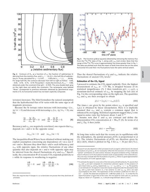
Fig. 3. The function g (blue squares) obtained by removing the memory flux from the 87 Sr 86 Sr data of Fig. 1, along with toc (red circles). Note that the range of the 87 Sr 86 Sr curve is approximately five times greater than in Fig. 1. The data are plotted such that the mean of both time series lies on the same horizontal line and their rms fluctuations have the same vertical extent. Thus the shared fluctuations of g and toc indicate the relative Fig. 2. Contours of R as a function of , the fraction of sedimentary Sr 0 and v w du u dw 0. [10] deriving from the memory flux, and t1 2 (ln 2), the half-life of sedimentary fluctuations of ancient CO 2 levels. Sr. R was calculated for 0, 0.01, ...,0.99 and t1 2 1,2,...,99My. For large half-life, the contours decrease from left to right as follow: 0.60, Estimation of the CO 2 Signal 0.65, 0.70, 0.75, 0.79. The symbol marks the minimum, R ** 0.80, obtained under the constraint that g(t) 0.7035. The area shaded dark gray I proceed to estimate the CO 2 signal explicitly. First, the highest on the right does not satisfy the constraint. The rectangular area labeled measurement of toc ,at175 My, is dropped because of its ‘‘Brass’’ corresponds to previous estimates obtained by geochemical arguments statistical insignificance (3). I then transform g(t) 3 g (t), a (17); its horizontal extent has not been explicitly computed. strontium-derived estimate of toc , by mapping the left axis of Fig. 3 to the corresponding value on the right axis. The quantities toc and g are then averaged to obtain terranes) increases. The third formalizes the natural assumption that the hydrothermal flux of Sr varies with the same sign as all t i g t i toc t i 2. [11] magmatic processes. Because the Sr isotope ratios increase with increasing r (i.e., The times t i are given by the points where toc is specified and g (t i ) is obtained by linear interpolation. Here it is implicitly gr 0) and decrease with increasing v h (i.e., gv h 0), one assumed that toc and g contain a common signal that is has enhanced by averaging. Statistical arguments suggest that ’srms signal-to-noise ratio lies between about 2 and 3.** g v g dv h v h dv 0 and g w g dr Assume now that and 0 are constant and define the 0. [8] dimensionless CO r dw 2 concentration 0 (8). In terms of and , Eq. 1 then yields Because g and toc are negatively correlated, one expects that toc depends on v and w in the opposite sense: 0 t 0 t . [12] toc v 0 and toc w 0. [9] At long time scales such that the oceans are in equilibrium with the atmosphere, the partial pressure pCO 2 is proportional to The inequalities 8 and 9 have been obtained without making any explicit assumption concerning any dependence of r on u nor (1). The relative fluctuations of pCO 2 are therefore given by (t)(0), which is plotted in Fig. 4 for 0 36 per mil (‰). on v and w. Because they show that v and w each influence g and toc with opposite signs, the relative fluctuations of any other quantity that also depends on v and w with opposite signs may Because can also depend on other processes b such as organic carbon burial, the shared fluctuations of g and toc do not necessarily reflect the full evolution of but rather the be inferred from the shared fluctuations of g and toc . Specifically, the concentration of oceanic CO 2 responds positively to v while its response to weathering is negative: ‘‘partial’’ contribution of v and w alone. However, the good correlation of Fig. 3 indicates that b’sinfluence on ’s fluctuations has been small, except possibly in the Carboniferous. Thus one may conclude that the fluctuations of g and toc follow to good approximation the fluctuations of with opposite signs. One also requires that if changes in v or w dominate one process then they dominate all processes. **To estimate the signal-to-noise ratio of the time series (t)defined by Eq. 11, assume that toc and g are each composed of a shared but unknown signal z in the presence of zero-mean noise toc and g, respectively: toc z toc and g z g. The quantity is an estimate of z. Its signal-to-noise ratio may be computed under the assumption that toc and g each have variance 2 , z has variance z 2 , and toc, g, and z are each uncorrelated to the other. The expectation of the correlation coefficient R is then z 2 ( z 2 2 ) (25). The observed correlation R 0.80 then yields z 2 2 4, or that the rms signal fluctuation is twice that of the noise. The rms signal-to-noise ratio of can be as large as a factor of 2 greater, i.e., it should range between about 2 and 3. GEOLOGY Rothman PNAS April 2, 2002 vol. 99 no. 7 4169
Page 1: Atmospheric carbon dioxide levels f
Page 5: 12. Derry, L. A. & France-Lanord, C

Atmospheric carbon dioxide levels for the last 500 million years

You also want an ePaper? Increase the reach of your titles

Delete template?

Save as template?