Kinetic Particles
Kinetic Particles
Kinetic Particles

You also want an ePaper? Increase the reach of your titles
YUMPU automatically turns print PDFs into web optimized ePapers that Google loves.
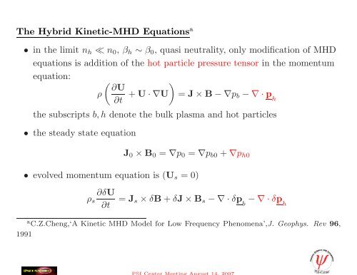
The Hybrid <strong>Kinetic</strong>-MHD Equations a<br />
• in the limit n h ≪ n 0 , β h ∼ β 0 , quasi neutrality, only modification of MHD<br />
equations is addition of the hot particle pressure tensor in the momentum<br />
equation:<br />
ρ<br />
( ∂U<br />
∂t + U · ∇U )<br />
= J × B − ∇p b − ∇ · p h<br />
the subscripts b, h denote the bulk plasma and hot particles<br />
• the steady state equation<br />
J 0 × B 0 = ∇p 0 = ∇p b0 + ∇p h0<br />
• evolved momentum equation is (U s = 0)<br />
ρ s<br />
∂δU<br />
∂t<br />
= J s × δB + δJ × B s − ∇ · δp b<br />
− ∇ · δp h<br />
1991<br />
a C.Z.Cheng,‘A <strong>Kinetic</strong> MHD Model for Low Frequency Phenomena’,J. Geophys. Rev 96,
Deposition of δp h<br />
onto Finite Element grid<br />
• assume CGL-like form δp h<br />
=<br />
⎛<br />
⎜<br />
⎝<br />
⎞<br />
δp ⊥ 0 0<br />
0 δp ⊥ 0 ⎟<br />
⎠<br />
0 0 δp ‖<br />
• evaluate pressure moment at a position x is<br />
δp ⊥ (x) =<br />
∫ 1<br />
2 mv2 ⊥δf(x,v)d 3 v<br />
=<br />
N∑<br />
i=1<br />
1<br />
2 mv2 i⊥g 0 w i δ 3 (x − x i )<br />
where sum is over the particles, m mass of the particle, g 0 w i is the<br />
perturbed phase density
The δf PIC method a b<br />
• PIC is a Lagrangian simulation of phase space f(x,v)<br />
• PIC evolves the f(x(t),v(t))<br />
• spatial grid is not inherantly necessary, but very convenient!<br />
• in principle, f(x(t),v(t)) contains everything<br />
• typically PIC is noisy, can’t beat 1/ √ N<br />
• δf PIC reduces the discrete particle noise associated with conventional PIC<br />
• Vlasov Equation<br />
z is the phase coordinate<br />
∂f(z)<br />
∂t<br />
+ ż · ∂f(z)<br />
∂z<br />
= 0<br />
a S. E. Parker and W. W. Lee, ‘A fully nonlinear characteristic method for gyro-kinetic<br />
simulation’, Physics of Fluids B, 5, 1993<br />
b G. Hu and J. A. Krommes, ”Generalized weighting scheme for δf particle simulation<br />
method”, Physics of Plasmas, 1, 1994
• split phase space distribution into steady state and evolving perturbation:<br />
f = f eq (z) + δf(z, t)<br />
• δf evolves along the characteristics ż (control variates MC c )<br />
using z = z eq + ˜z and ż eq · ∂f eq<br />
∂z = 0<br />
˙ δf = −˜z · ∂f eq<br />
∂z<br />
• the drift kinetic equations of motion are used as the particle characteristics<br />
ẋ = v ‖ˆb + m (<br />
)<br />
eB 4 u 2 + v2 ⊥<br />
)(B × ∇ B2<br />
+ E × B<br />
2 2 B 2 + µ 0mv‖<br />
2<br />
eB 2 J ⊥<br />
m˙v ‖ = −ˆb · (µ∇B − eE)<br />
c A. Y. Aydemir, ”A unified MC interpretation of particle simulations...”, Physics of Plasmas,<br />
1, 1994
Slowing Down Distribution for Hot <strong>Particles</strong><br />
• for the slowing down distribution function<br />
f eq = P 0 exp( P ζ<br />
ψ 0<br />
)<br />
ε 3/2 + ε 3/2<br />
0<br />
where P ζ = gρ ‖ − ψ is the canonical toroidal momentum and ε is the<br />
energy, ψ 0 is the total flux, and ε c is the critical slowing down energy<br />
{ [( )<br />
]<br />
δf ˙ mg<br />
= f eq<br />
eψ 0 B 3 v‖ 2 + v2 ⊥<br />
δB · ∇B − µ 0 v ‖ J · E<br />
2<br />
}<br />
where<br />
+ δv · ∇ψ p<br />
ψ 0<br />
+ 3 2<br />
eε 1/2<br />
ε 3/2 + ε 3/2<br />
0<br />
v D · E<br />
v D = m ( )<br />
v 2<br />
eB 3 ‖ + v2 ⊥<br />
(B × ∇B) + µ 0mv‖<br />
2<br />
2<br />
eB J 2 ⊥<br />
δv =<br />
E × B<br />
B 2 + v ‖ · δB B
Benchmark with M3D<br />
• improved particle loading - ensures velocity space isotropy<br />
• velocity shows most activity in the most energetic particles<br />
• mostly in trapped region, also in extremes of passing particles
0.4<br />
0.3<br />
0.3<br />
0.2<br />
0.2<br />
0.1<br />
0.1<br />
Z [m]<br />
0.0<br />
Z [m]<br />
0.0<br />
-0.1<br />
-0.1<br />
-0.2<br />
-0.2<br />
-0.3<br />
-0.3<br />
-0.4<br />
0.6 0.7 0.8 0.9 1.0 1.1 1.2 1.3 1.4<br />
R [m]<br />
0.7 0.8 0.9 1.0 1.1 1.2 1.3<br />
R [m]<br />
• simulations without anisotropy reproduce ideal MHD with γ within 10%<br />
• no real frequency<br />
• anisotropic pressure ∆p = p ‖ − p ⊥ is key to energetic effects
0.3<br />
0.3<br />
0.2<br />
0.2<br />
0.1<br />
0.1<br />
Z [m]<br />
0.0<br />
Z [m]<br />
0.0<br />
-0.1<br />
-0.1<br />
-0.2<br />
-0.2<br />
-0.3<br />
-0.3<br />
0.6 0.7 0.8 0.9 1.0 1.1 1.2 1.3 1.4<br />
R [m]<br />
0.7 0.8 0.9 1.0 1.1 1.2 1.3<br />
R [m]<br />
• simulations with only passing particles stabilize but do not change V φ mode<br />
topology<br />
• trapped particles excite precessional fishbone mode (plot on right)
• for β frac > 25% simulations with only passing particles entirely stable<br />
γ ∼ 0<br />
• with only trapped particles v cutoff = 1.e6, γ > γ ideal .<br />
• with only trapped particles v cutoff = 1.5e6, γ < γ ideal .<br />
• inclusion of more energetic trapped particles has stabilizing influence - in<br />
line with prevailing ideas of energetic particle effects on (1, 1)<br />
• at larger v cutoff (stronger anisotropy) there exists a window of stability<br />
• modest energy passing particles seem to stabilize (1, 1)!
Linear Simulations of Tearing Modes in a RFP<br />
[ ( r α0<br />
]<br />
• alpha model equilibrium ∇ × B = µB µ = 2Θ 1 −<br />
a)<br />
• parameters for straight cylinder<br />
a = .5m, B 0 = .3T, Θ = 1.75, α 0 = 3,<br />
S = 1.e4, ka = 2, γτ A = 1.3e − 3<br />
• Boris push with orbit averaging to accommodates disparate time scales<br />
[<br />
• energetic ion density profile ∝ exp − ( ) ]<br />
r 2<br />
0.45a<br />
• initialize with mono-energetic particles δ(v ⊥ − v 0 ), only v × δB in weight<br />
equation<br />
• use only perpendicular pressure for comparison with theory<br />
• subcyling of particles and orbit average particle pressure
δf and the Lorentz Equations<br />
• Lorentz equation of motion<br />
ẋ = v<br />
˙v = q m<br />
(E + v × B)<br />
• for Lorentz equations use a<br />
f eq = f 0 (x, v 2 ) + 1 ω c<br />
(v · b × ∇f 0 )<br />
• weight equation is<br />
δf ˙<br />
δE + v × δB<br />
= −<br />
B<br />
· b × ∇f 0 − 2q<br />
m δE · v∂f 0<br />
∂v 2<br />
a M. N. Rosenbluth and N. Rostoker “Theoretical Structure of Plasma Equations”, Physics<br />
of Fluids 2 23 (1959)
FLR Stabilization of RFP Tearing Mode<br />
• stabilization with increasing v ⊥<br />
v 0 (m/s) L/a γτ A<br />
base case - 1.3 × 10 −3<br />
1.0 × 10 6 .14 1.0 × 10 −3<br />
1.5 × 10 6 .21 5.4 × 10 −4<br />
2.0 × 10 6 .28 1.5 × 10 −4<br />
2.5 × 10 6 .35 5.1 × 10 −5<br />
• stabilization at L/a ≃ 1/3, where L is the Larmor diameter
FLR Broadens Tangential Velocity Eigenmode Structure<br />
1.0<br />
w/ FLR<br />
w/o FLR<br />
1.0<br />
w/ FLR<br />
w/o FLR<br />
0.8<br />
0.5<br />
0.6<br />
normalized units<br />
0.0<br />
normalized units<br />
0.4<br />
0.2<br />
-0.5<br />
0.0<br />
-0.2<br />
-1.0<br />
0.0 0.1 0.2 0.3 0.4 0.5<br />
minor radius [m]<br />
-0.4<br />
0.0 0.1 0.2 0.3 0.4 0.5<br />
minor radius [m]<br />
• tangential velocity eigenmode substantially altered (left)<br />
• magnetic eigenmode unaltered (right)
Comparison of V φ Eigenmode<br />
0.4<br />
0.4<br />
0.2<br />
0.2<br />
Z<br />
0.0<br />
Z<br />
0.0<br />
-0.2<br />
-0.2<br />
-0.4<br />
-0.4<br />
1.6 1.8 2.0 2.2 2.4<br />
R<br />
1.6 1.8 2.0 2.2 2.4<br />
R<br />
• inner circle shows resonance surface
The Future<br />
• impact of localization of density<br />
• full velocity distribution<br />
• obtain MST equilibria and examine toroidicity - trapped particles<br />
• visit in Sept-Oct