
You also want an ePaper? Increase the reach of your titles
YUMPU automatically turns print PDFs into web optimized ePapers that Google loves.
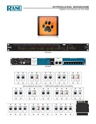
<strong>RaneNote</strong><br />
AUDIO IN HOUSES OF WORSHIP<br />
Audio in Houses of Worship<br />
• Common Signal Processing Blocks<br />
• Specific Examples<br />
Michaël Rollins<br />
Rane Corporation<br />
<strong>RaneNote</strong> 162<br />
© 2006 Rane Corporation<br />
Introduction<br />
Audio is an essential element in any modern-day<br />
religious service. What is heard by the congregation<br />
is a combination of the acoustic qualities of the room<br />
and the performance of the audio system. Some of the<br />
desirable acoustic qualities in a house of worship are:<br />
Reverberance – when well controlled with early decay,<br />
the effect is perceived as a beautiful sound that<br />
enhances the quality of the audio. See the Rane Pro<br />
Audio Reference for a definition of “reverberation.”<br />
Clarity – is the ratio of the energy in the early sound<br />
compared to that in the reverberant sound. Early<br />
sound is what is heard in the first 50 - 80 milliseconds<br />
after the arrival of the direct sound. It is a measure<br />
of the degree to which the individual sounds<br />
stand apart from one another.<br />
Articulation – is determined from the direct-to-total<br />
arriving sound energy ratio. When this ratio is small,<br />
the character of consonants is obscured resulting in<br />
a loss of understanding the spoken word.<br />
Listener envelopment – results from the energy of the<br />
room coming from the sides of the listener. The effect<br />
is to draw the listener into the sound.<br />
Where a conference room would be optimized for<br />
articulation and clarity, a symphony hall is optimized<br />
for reverberance and listener envelopment. A good<br />
house of worship is optimized as a compromise between<br />
the somewhat conflicting requirements of music<br />
performance and the spoken word. Articulation must<br />
be excellent but sufficient reverb is required to complement<br />
music performances. All reflections must be well<br />
controlled to achieve this balance and ensure the best<br />
possible listener experience.<br />
Epcot is a registered trademark of Disney Enterprises, Inc.<br />
Band-Aid is a registered trademark of Johnson & Johnson Consumer Companies, Inc.<br />
Houses of Worship-
An Example of Good Sound<br />
There are other possible examples but the author really<br />
likes this one. In some mosques, cathedrals and<br />
tabernacles there are wonderful low-domed ceilings<br />
that have marvelous natural acoustic properties. The<br />
acoustic coupling from performers to the congregation<br />
grouped under the dome makes for a very (dare I say)<br />
“spiritual” experience. For the purpose of this article,<br />
this level of performance is a “gold standard” to which<br />
other acoustic spaces will be compared in the search<br />
for improvements and recommendations.<br />
The U.S.A. Pavilion at Florida’s Epcot® Center makes<br />
for an interesting case study. There is a dome ceiling<br />
in the pavilion. Under the dome an eight-part acappella<br />
group called the “Voices of Liberty” performs. For<br />
those under the dome listening to the group, the sound<br />
is beautiful and inspiring. Moving out from under the<br />
dome, the “magic” is gone.<br />
This level of performance is not feasible in a typical<br />
house of worship but it does establish an icon as to<br />
what could be if there was sufficient skill (and budget)<br />
applied to the acoustic and audio system design.<br />
And Now The Ugly World in Which We Live<br />
Contrast this to a typical public address system<br />
squawking bad sound to the congregation. That which<br />
was good is replaced with misery. You reach for a bottle<br />
of aspirin to calm the headache induced by a pair of<br />
blaring powered speakers.<br />
Some of the problems encountered by audio designers/consultants<br />
include:<br />
Excessive Reverberation – such that articulation and<br />
clarity is poor.<br />
Echo – where a discrete sound reflection returns to a<br />
listener more then 50 milliseconds from the direct<br />
sound and is significantly louder then the reverberation<br />
sound.<br />
Flutter echo – repeated echoes that are experienced<br />
in rapid succession that occur between two hard<br />
parallel surfaces. All echoes ruin the acoustic properties<br />
of a room and a flutter echo is particularly<br />
damaging.<br />
Coloration due to reflections – when a reflection destructively<br />
recombines with the direct sound modifying<br />
the frequency response in the process. These<br />
are non-minimum-phase colorations as correction<br />
with equalization is not possible.<br />
Delayed Sound – from coupled volumes (contamination<br />
from adjacent rooms storing sound energy and<br />
then returning the energy to the main room).<br />
Psychological preconditioning – It is a common<br />
problem for the clergy and congregation to be so<br />
preconditioned by bad sound that they become resistant<br />
to change and find it difficult to (at first) recognize<br />
good sound. This can also work in the audio<br />
consultants favor when the customers are preconditioned<br />
by good sound and are willing to invest the<br />
required resources toward good audio design.<br />
For those of us designing audio for houses of worship<br />
with a rectangular room, flat walls and probably<br />
a vaulted ceiling, some form of sound reinforcement<br />
is required. Through attention to detail and careful<br />
design of the audio system, the experience of the congregation<br />
can be non-aspirin inducing and the system<br />
simple to use.<br />
Common Signal Processing Blocks<br />
Let’s begin by looking at the universal signal processing<br />
chain common to all audio systems. In the simplest<br />
systems these functions are accomplished in an audio<br />
mixer that feeds a pair of powered speakers. More sophisticated<br />
systems include equalization, compression,<br />
limiting, automation, feedback suppression, electronic<br />
crossovers and other tools of the trade. These days it<br />
is possible to include all of these functions in a DSP<br />
(Digital Signal Processor). One example of the signal<br />
chain from the minister’s microphone to the power<br />
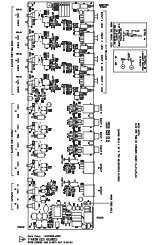
amplifiers is shown in Figure 1.<br />
Houses of Worship-<br />
Figure 1. Microphone to Amplifier Chain
The signal processing flow starts at the Analog Input.<br />
A 2-band Parametric Equalizer filters out-of-band<br />
low frequencies. The microphone signals are summed<br />
together in an Automatic Mixer. An AGC (Automatic<br />
Gain Control) reduces the dynamic range and a High-<br />
Pass Filter in the side chain improves the performance<br />
of the AGC. The Level control can be tied to a pot on<br />
the wall or a smart remote. There is a Feedback Suppressor<br />
for good measure. A 2-way Crossover supports<br />
a biamplified system. The 10-band Parametric Equalizers<br />
are utilized for both wide- and narrow-band corrections.<br />
Generally, wide-band filters correct minimumphase<br />
frequency response irregularities in the speaker<br />
drivers and in the room response. Narrow-band filters<br />
are useful to partially correct non-minimum-phase<br />
related problems such as energy stored in room modes<br />
(reverberant energy). A Limiter could also have been<br />
added to protect the system from clipping if that feature<br />
is not included in the power amplifier.<br />
Now let’s take a look at some of these signal processing<br />
blocks in greater detail.<br />
maximum SNR (Signal to Noise Ratio). Your exercise is<br />
to determine why the SNR was only degraded by 8 dB<br />
rather then the intuitively obvious value of 13 dB.<br />
Answer: The noise floor does drop by 13 dB, but this<br />
combination of settings causes the analog input stage<br />
to clip at an input level that is 5 dB lower. Hence, the<br />
change in system SNR is 8 dB.<br />
Applying attenuation after the input stage (rather<br />
then gain) reduces overload performance and so should<br />
be used with skill and discretion. It is the proper technique<br />
to maximize noise performance.<br />
For more detailed technical information please see<br />
the <strong>RaneNote</strong> “Selecting Mic Preamps.”<br />
Analog Input / Microphone Preamp<br />
It is surprising how often even experienced audio<br />
consultants will configure an audio input incorrectly.<br />
It is important that as much gain as possible is accomplished<br />
at the front end of the system in the Analog<br />
Gain stage. Any additional gain from Digital Trim<br />
after the input stage degrades optimum signal-to-noise<br />
performance.<br />
Figure 2. Drag Net Input Block<br />
As an example, let’s set the input gain to a value of<br />
+40 dB. One way is where the analog gain is set to a<br />
value of +45 dB and the<br />
digital trim is set to -5 dB<br />
(as in Figure 2), the measured<br />
input referred noise<br />
is -127 dBu. A common<br />
(but incorrect) way would<br />
have the analog gain set to<br />
a value of +30 dB and the<br />
digital trim set to +10 dB<br />
(the author has seen this<br />
repeatedly), to give the<br />
same Mic gain of 40 dB —<br />
but now the input-referred<br />
noise is degraded to -114<br />
dBu. That is an increase of<br />
13 dB for the noise floor,<br />
or a change (in the bad<br />
direction) of 8 dB in the<br />
Figure 3. Drag Net Parametric EQ for Input Low Cut<br />
Houses of Worship-
Input Low-Cut Filter<br />
A very good idea is to add<br />
a low-cut filter set to ~80<br />
Hz after the input stage<br />
to minimize the effects of<br />
undesirable low-frequency<br />
noises such as bumps and<br />
thumps that come from<br />
handling the mic and also<br />
wind blasts and pops from<br />
speaking too closely into<br />
the microphone. In Figure<br />
3, both 2nd-order filters are<br />
set to the same frequency to<br />
produce a 4th-order filter.<br />
There should also be a<br />
low-cut filter in line with<br />
Figure 4. Drag Net Parametric for AGC Side Chain<br />
the SC (Side Chain) input<br />
of the AGC (Automatic Gain Control). This filter can<br />
be set to a higher corner frequency (such as 120 Hz in<br />
Figure 4) to improve the performance of the AGC by<br />
rejecting the effects of low frequency noises.<br />
The Auto Mixer —<br />
A Little Automation Buddy<br />
An Auto Mixer (shown in Figure 5) is a good<br />
idea when there is more then a single open<br />
microphone. Auto Mixers combine the signals<br />
from multiple microphones and automatically<br />
correct for the changing gain requirements<br />
as the NOM (Number of Open Microphones)<br />
changes.<br />
Threshold with Last On is a useful setting<br />
for all microphones used in a worship service<br />
(Figure 6). Unused microphones (input levels<br />
are below threshold) are gated. When the input<br />
of a microphone is above threshold then other<br />
inputs with a lower assigned priority level are ducked.<br />
Figure 5. Drag Net Auto Mixer Block<br />
Automatic Gain Control<br />
A Compressor is the correct processing block in this<br />
link of the audio chain. Something is needed here to<br />
prevent exuberant preaching from melting down the<br />
congregation. Surprisingly, an AGC can be very useful<br />
in this position but configured to behave more like a<br />
specialized compressor by using the settings shown in<br />
Figure 7.<br />
Houses of Worship-<br />
Figure 6. Auto Mixer Input Edit Block
The value of “Threshold<br />
re: Target” is set to<br />
have an offset of 0 dBr<br />
so that “Threshold” has<br />
the same value as the<br />
“Target.” “Maximum<br />
Gain” becomes 0 dB and<br />
the gain curve starts<br />
to look like a compressor<br />
but there are additional<br />
controls in<br />
an AGC for Hold and<br />
Release that are useful when the input level is below<br />
threshold. These settings avoid the problems of compressor<br />
“pumping” when that exuberant speaker is at<br />
the microphone as attenuation levels are held between<br />
spoken phrases. Then, when transitioning to a more reserved<br />
speaker, the hold time (below threshold) is short<br />
enough to expire so that the gain returns to a normal<br />
level.<br />
Figure 7. Drag Net AGC Block<br />
An Exciting Labor-Saving Tip —<br />
Put a Control On the Wall<br />
A level control can provide attenuation as needed under<br />
the control of a pot on the wall or a smart remote.<br />
This is handy in systems where a minister needs to run<br />
a system alone without the assistance of an audio specialist<br />
who is running a mixing board. The remote can<br />
be located on or close to a pulpit which places control<br />
of the audio system at the fingertips of the minister.<br />
The DSP control is shown in Figure 8.<br />
Figure 8a. Drag Net Level<br />
Block Mapped to a Remote<br />
Level Control<br />
Figure 8b. You can mount<br />
a 20 kΩ pot anywhere, or<br />
Rane makes a remote that<br />
fits in any standard U.S.<br />
electrical box and can be<br />
covered with a Decora<br />
plate cover.<br />
Houses of Worship-
Figure 9. Drag Net Feedback Suppressor<br />
Feedback Suppression — A Gift From Above?<br />
The next item in this processing chain is somewhat controversial.<br />
It is a Feedback Suppressor. To some audio consultants<br />
a Feedback Suppressor is heresy! The argument<br />
is that a properly calibrated system has no need of such<br />
a Band-Aid®. This is generally true, but there is one case<br />
when it is wise for an audio consultant to suffer the ignominy<br />
of using a Feedback Suppressor — a lay clergy where<br />
the person speaking is untrained and/or unfamiliar with<br />
proper use of a microphone. The author has witnessed<br />
such a person cup their hands (in the attitude of prayer)<br />
directly around the microphone capsule. The hands form<br />
a resonant chamber that results in squealing feedback. A<br />
good Feedback Suppressor would have locked on to the<br />
offending tone and notched it out posthaste.<br />
Using Auto Setup to<br />
ring out a system<br />
1. Setup the system's gain<br />
structure.<br />
2. Umute the mic(s).<br />
3. Talk into the mic(s) and<br />
adjust the system gain<br />
until it is on the verge of<br />
feedback.<br />
4. Click Auto Setup to<br />
automatically deploy<br />
Fixed filters as feedback<br />
occurs.<br />
Auto Setup deploys<br />
unused (flat) Fixed filters.<br />
Once Auto Setup is<br />
complete, Floating filters<br />
are deployed should<br />
feedback occur.<br />
Houses of Worship-
Parametric Equalization: Now We’re Having Real Fun<br />
Parametric equalizers are<br />
used for both wide and narrow<br />
band corrections. Generally,<br />
wide-band and shelf filters can<br />
correct for minimum-phase frequency<br />
response irregularities.<br />
One interesting detail of Figure<br />
10 is Hi-Shelf Filter 1. This<br />
filter was added after achieving<br />
flat in-room response. Since<br />
the system was calibrated in an<br />
empty room, this extra highfrequency<br />
energy is intended<br />
to compensate for the highfrequency<br />
absorption of the<br />
congregation when the room<br />
is full of people. There is also a<br />
noise-masking effect in some<br />
congregations that will tend to<br />
obscure the intelligibility of the<br />
spoken word. In practice this<br />
approach of adding a bit of extra<br />
high-frequency energy into<br />
Figure 10. Drag Net Parametric Block (May Have up to 15 Bands per Block)<br />
the room works well.<br />
Narrow-band filters (Figure<br />
11) are useful to partially<br />
correct non-minimum-phase<br />
related problems such as energy<br />
stored in room modes. At low<br />
frequencies this energy causes<br />
bass to sound indistinct, and in<br />
midrange to lower treble this<br />
energy is perceived as reverberation.<br />
These filters attenuate<br />
the frequencies bouncing about<br />
the room. In an acoustically<br />
live room, room resonances<br />
can propagate for a surprisingly<br />
long time causing these frequencies<br />
to “build up.” Narrowband<br />
filters are just a partial<br />
solution. Greatest effectiveness<br />
is achieved when filters are used<br />
in conjunction with acoustic<br />
room treatments such as diffusers,<br />
high/mid frequency absorbers<br />
and bass traps. This topic is<br />
Figure 11. Parametric with Narrow-Band Filters<br />
beyond the scope of this Rane-<br />
Note but an important part of<br />
the audio consultant’s craft.<br />
Houses of Worship-
Specific Examples<br />
Example #1: A Small Church<br />
Description<br />
The ceiling is low suspended acoustic tile over an open<br />
space covered with thin carpet. The RT60 (the time it<br />
takes the reverberant sound to decrease by 60 dB) is<br />
short, so controlling reverberation is not a problem. In<br />
fact, the room is a touch “dry” for music, and content<br />
of the worship service includes live music performances.<br />
Audio sources are the minister’s wireless microphone,<br />
the band, a DVD/CD player and other devices<br />
as needed. Control is via a 24-channel mixer with all<br />
inputs used. Output is to a pair of powered speakers<br />
mounted high in the room corners in a stereo configuration.<br />
This installation was done by members of the<br />
congregation without professional audio consultation.<br />
Problems<br />
• The quality of the audio is poor with numerous<br />
problems including uneven frequency response.<br />
• An experienced sound person is required to run the<br />
mixer for all audio system use.<br />
• There is poor congregation coverage from the stereo<br />
speaker pair. People sitting in the hot spots just in<br />
front of the speakers are blasted with excessive level,<br />
and the rest of the congregation is exposed to a<br />
strong interference pattern between the two speakers.<br />
The system is uncompensated for room modes,<br />
room response and speaker response irregularities.<br />
There is a small “sweet spot” in the center of the<br />
room where the two speakers combine coherently<br />
but there is an isle down the center. Since there are<br />
no chairs, no one is seated in the “sweet spot”.<br />
So does this audio system work the way it is? Yes,<br />
but even the pastor knows the congregation may not be<br />
receiving the best possible audio experience.<br />
Recommendations<br />
Improvements to this system are accomplished in<br />
a number of ways. A DSP can be used for equalization,<br />
other processing and to add automation to the<br />
minister’s microphone. The entire worship band could<br />
be run through a mixer with each individual input<br />
processed by an AGC. There are admittedly downsides<br />
to automating the audio mixing of a large group, as<br />
the automation is not as intelligent as an experienced<br />
sound person, but is possible in some cases.<br />
The speaker system is examined for options providing<br />
more even coverage of the congregation. Improvements<br />
can be introduced in phases.<br />
Houses of Worship-<br />
STAGE<br />
FOH MIXER<br />
Figure 12. Stereo Speaker Pair Coverage<br />
Phase 1<br />
Add a DSP box between the mixer output and main<br />
speakers and on-stage monitors. Features added could be:<br />
• Parametric Wide-Band Equalization. This alone<br />
would greatly improve this system.<br />
• Parametric Narrow-Band Equalization. A short<br />
RT60 makes this unnecessary at this time. However,<br />
remodeling could increase RT60 to where narrowband<br />
equalization would be needed. (This room<br />
could use bass absorbers).<br />
• High-Pass Filtering. If not already in the mixer.<br />
• Compression. Always a good idea with microphones<br />
because of the inverse square law relationship between<br />
the preacher’s mouth and the location of the<br />
microphone. See the Rane Pro Audio Reference entry<br />
for “Inverse Square Law.”<br />
• Feedback Suppression. If needed.<br />
Phase 2<br />
Automation is incorporated with automixers and<br />
remote controls. There are many exciting ways to add<br />
these features depending on the congregation needs.<br />
The most obvious upgrade is to add the ability for a<br />
minister to turn on and control the main microphones<br />
from a simple control panel in easy reach at the stage.<br />
Phase 3<br />
The very uneven coverage of the congregation by the<br />
stereo speaker pair needs to be addressed as shown in<br />
Figure 12. The seats directly in front of the speakers<br />
have enough level to kill small animals.<br />
If the audio system were perfect then each seat in
STAGE<br />
STAGE<br />
FOH MIXER<br />
FOH MIXER<br />
Figure 13. Line Array Speaker Coverage<br />
the congregation would have the same audio level. In<br />
the author’s experience, similar rooms have been controlled<br />
within a couple of dB. In this example, the seat<br />
closest to each loudspeaker is about 15 dB louder then<br />
the worst seat on the floor, and interference between<br />
the two speakers adds to a very lumpy and unpleasant<br />
frequency response. The FOH (Front Of House) Mixer<br />
is placed in a location for good sound, causing the levels<br />
at the ends of the front rows to be way too loud.<br />
Line Array Speakers<br />
One improvement is to remove the stereo pair of pointsource<br />
loudspeakers and install a line array located<br />
in the center of the back wall as shown in Figure 13.<br />
Coverage of the congregation is more even, and the<br />
level at the FOH Mixer location is very similar to the<br />
coverage level over the whole floor of the congregation.<br />
The level of the stage monitors is greatly reduced and<br />
may no longer be needed by the musicians. Within the<br />
near field of the line array there is a range were the audio<br />
level will decrease by only 3 dB for each doubling of<br />
distance which greatly helps even the coverage across<br />
the entire floor. The audio is distributed across the<br />
whole line so that even if a microphone is right next to<br />
the array, there is little tendency to feedback.<br />
In this example, there is a low suspended acoustic<br />
tile ceiling that shortens the length of a line array<br />
speaker. This limits the mounting options and the<br />
maximum length of a line array so this might not be<br />
the best solution. If the room were remodeled so there<br />
was a high ceiling, then a line array would fit. This<br />
is especially true if the newly remodeled ceiling was<br />
Figure 14. Distributed Array Speaker Coverage<br />
acoustically reflective causing the RT60 of the room<br />
to be much greater. The high directivity of a long line<br />
array greatly helps to project the audio out to the floor<br />
rather then have the audio directed toward the ceiling<br />
where it contributes to the reverberant energy and<br />
echoes in the room.<br />
Supplemental Distributed Array Speakers<br />
Because of the dropped ceiling, another option is a distributed<br />
array of supplemental ceiling speakers in the<br />
back of the room as shown in Figure 14. The loudness<br />
level of the main stereo pair could be reduced by at<br />
least 12 dB. This would greatly diminish the hot spots<br />
in the front, but would leave the level at the back way<br />
too low. Ceiling speakers can be added in the locations<br />
shown to fill in the audio in the back of the room.<br />
It is important to include a speaker over the mixer<br />
location so the audio at that location matches the level<br />
in the congregation to acheive an accurate mix.<br />
Why The Delay?<br />
The ceiling loudspeaker signals should be time delayed<br />
so their output combines coherently with the pointsource<br />
pair in the front of the room. If the rear loudspeakers<br />
are not correctly delayed then the loudspeakers<br />
in the room will not combine correctly.<br />
This room is too small for audio from the front of<br />
the room to be perceived as a distinct echo. Applying<br />
delay to the ceiling speakers can minimize the problem<br />
of localization confusion occuring if the first arrival<br />
sound is coming from the overhead loudspeakers and<br />
not the front of the room.<br />
Houses of Worship-
Example #2: A Mid-Sized Contemporary<br />
House of Worship<br />
Description<br />
This second example is a medium sized house of worship.<br />
The vaulted ceiling is high and the floor in the<br />
congregational seating area is covered with hard vinyl.<br />
The RT60 is approximately 1.5 seconds so reverberation<br />
is a problem in an empty room. The sources of audio<br />
are ministers on a microphone and a worship band.<br />
Control is via a 32-channel mixer. The speaker system<br />
is an array of three large boxes mounted as a central<br />
cluster high in the peak of the ceiling. A professional<br />
audio company did the installation and calibration.<br />
The quality of the audio in this church is much better<br />
than in the first example. An interesting question is:<br />
how good is “good enough”? When interviewed, members<br />
of this congregation can usually hear. Rarely is the<br />
audio painful to listen to, so some say that the audio<br />
quality is fully acceptable. Reflect back on the example<br />
in the introduction where domed ceilings were held up<br />
as an icon of natural acoustic wonderfulness. Let’s see<br />
how this audio system installation stacks up.<br />
Problems<br />
• Reverberance is not controlled and is dependent<br />
on the configuration and occupancy of the room.<br />
Low-mid frequencies are a particular problem as the<br />
energy builds up and is never trapped.<br />
• Clarity is fairly good, meeting a minimum standard.<br />
• Articulation is acceptable but not outstanding. The<br />
ALCONs (Articulation Loss of Consonants) rating<br />
of this room is fairly low but in the acceptable range.<br />
However, there is room for improvement.<br />
• Listener envelopment is nonexistent and pales in<br />
comparison to the example of a domed ceiling.<br />
• As in the first example, an experienced sound person<br />
is required to run the mixer for any use of the audio<br />
system, as there is no system automation.<br />
• There is good coverage of the congregation from the<br />
central cluster, but people sitting in the area where<br />
the coverage patterns between two of the speakers<br />
overlap experience uneven frequency response<br />
due to the comb filtering caused by the interference<br />
between these two speakers.<br />
• Bass response is particularly poor. The poor bass response<br />
leads to the impression that the system lacks<br />
sufficient power.<br />
Houses of Worship-10<br />
STAGE<br />
FOH<br />
MIXER<br />
Figure 15. Distributed Array Speaker Coverage<br />
Recommendations<br />
A DSP unit is already in the system and can be used<br />
for additional equalization and other tasks. The same<br />
recommendation applies to add enough automation so<br />
that a simple service can be done without bringing in a<br />
sound person.<br />
The speaker system may already be fully adequate.<br />
The first temptation may be to add a subwoofer, but it is<br />
probable that the buildup of mid-bass energy makes the<br />
bass quality so poor that adding more will only make<br />
matters worse. To fix the room, the ceiling and walls<br />
could be covered in bass absorptive panels, but this is<br />
not practical. A compromise is to add bass traps to the<br />
room corners and the ceiling ridge.<br />
If it is not possible to tame the room with traps, narrow-band<br />
filtering techniques could solve things. The<br />
room is evaluated for the modes that build up room energy<br />
and these frequencies are notched out with a very<br />
narrow filter. A combination of some absorptive panels<br />
and narrow-band filters might be the best compromise.<br />
There are regions (as shown in Figure 15) where the<br />
coverage from the individual speakers in the cluster<br />
interfere with each other rather than combine cooperatively.<br />
This interference is frequency-dependent. The<br />
solution is to reduce the contribution of some of the<br />
speakers of those problem frequencies so that interference<br />
is minimized.<br />
The system would then require re-calibration to<br />
complement the above changes. That should do it.<br />
©Rane Corporation 10802 47th Ave. W., Mukilteo WA 98275-5098 USA TEL 425-355-6000 FAX 425-347-7757 WEB www.rane.com
<strong>RaneNote</strong><br />
AUDIO SPECIFICATIONS<br />
Audio Specifications<br />
• Audio Distortion<br />
• THD - Total Harmonic Distortion<br />
• THD+N - Total Harmonic Distortion + Noise<br />
• IMD – SMPTE - Intermodulation Distortion<br />
• IMD – ITU-R (CCIF) - Intermodulation Distortion<br />
• S/N or SNR - Signal-To-Noise Ratio<br />
• EIN - Equivalent Input Noise<br />
• BW - Bandwidth or Frequency Response<br />
• CMR or CMRR - Common-Mode Rejection<br />
• Dynamic Range<br />
• Crosstalk or Channel Separation<br />
• Input & Output Impedance<br />
• Maximum Input Level<br />
• Maximum Output Level<br />
• Maximum Gain<br />
• Caveat Emptor<br />
Introduction<br />
Objectively comparing pro audio signal processing<br />
products is often impossible. Missing on too many data<br />
sheets are the conditions used to obtain the published<br />
data. Audio specifications come with conditions. Tests<br />
are not performed in a vacuum with random parameters.<br />
They are conducted using rigorous procedures<br />
and the conditions must be stated along with the test<br />
results.<br />
To understand the conditions, you must first understand<br />
the tests. This note introduces the classic<br />
audio tests used to characterize audio performance.<br />
It describes each test and the conditions necessary to<br />
conduct the test.<br />
Apologies are made for the many abbreviations,<br />
terms and jargon necessary to tell the story. Please<br />
make liberal use of Rane’s Pro Audio Reference (www.<br />
rane.com/digi-dic.html) to help decipher things. Also,<br />
note that when the term impedance is used, it is assumed<br />
a constant pure resistance, unless otherwise<br />
stated.<br />
The accompanying table (back page) summarizes<br />
common audio specifications and their required conditions.<br />
Each test is described next in the order of appearance<br />
in the table.<br />
Dennis Bohn<br />
Rane Corporation<br />
<strong>RaneNote</strong> 145<br />
© 2000 Rane Corporation<br />
Audio Specifications-
Audio Distortion<br />
By its name you know it is a measure of unwanted<br />
signals. Distortion is the name given to anything that<br />
alters a pure input signal in any way other than changing<br />
its magnitude. The most common forms of distortion<br />
are unwanted components or artifacts added to<br />
the original signal, including random and hum-related<br />
noise. A spectral analysis of the output shows these<br />
unwanted components. If a piece of gear is perfect the<br />
spectrum of the output shows only the original signal<br />
– nothing else – no added components, no added<br />
noise – nothing but the original signal. The following<br />
tests are designed to measure different forms of audio<br />
distortion.<br />
THD. Total Harmonic Distortion<br />
What is tested? A form of nonlinearity that causes unwanted<br />
signals to be added to the input signal that are<br />
harmonically related to it. The spectrum of the output<br />
shows added frequency components at 2x the original<br />
signal, 3x, 4x, 5x, and so on, but no components at,<br />
say, 2.6x the original, or any fractional multiplier, only<br />
whole number multipliers.<br />
How is it measured? This technique excites the unit<br />
with a single high purity sine wave and then examines<br />
the output for evidence of any frequencies other than<br />
the one applied. Performing a spectral analysis on<br />
this signal (using a spectrum, or FFT analyzer) shows<br />
that in addition to the original input sine wave, there<br />
are components at harmonic intervals of the input<br />
frequency. Total harmonic distortion (THD) is then<br />
defined as the ratio of the rms voltage of the harmonics<br />
to that of the fundamental component. This is accomplished<br />
by using a spectrum analyzer to obtain the<br />
level of each harmonic and performing an rms summation.<br />
The level is then divided by the fundamental level,<br />
and cited as the total harmonic distortion (expressed<br />
in percent). Measuring individual harmonics with<br />
precision is difficult, tedious, and not commonly done;<br />
consequently, THD+N (see below) is the more common<br />
test. Caveat Emptor: THD+N is always going to be a<br />
larger number than just plain THD. For this reason,<br />
unscrupulous (or clever, depending on your viewpoint)<br />
manufacturers choose to spec just THD, instead of the<br />
more meaningful and easily compared THD+N.<br />
Required Conditions. Since individual harmonic<br />
amplitudes are measured, the manufacturer must state<br />
the test signal frequency, its level, and the gain conditions<br />
set on the tested unit, as well as the number of<br />
harmonics measured. Hopefully, it’s obvious to the<br />
reader that the THD of a 10 kHz signal at a +20 dBu<br />
level using maximum gain, is apt to differ from the<br />
THD of a 1 kHz signal at a -10 dBV level and unity<br />
gain. And more different yet, if one manufacturer measures<br />
two harmonics while another measures five.<br />
Full disclosure specs will test harmonic distortion<br />
over the entire 20 Hz to 20 kHz audio range (this is<br />
done easily by sweeping and plotting the results), at<br />
the pro audio level of +4 dBu. For all signal processing<br />
equipment, except mic preamps, the preferred gain setting<br />
is unity. For mic pre amps, the standard practice<br />
is to use maximum gain. Too often THD is spec’d only<br />
at 1 kHz, or worst, with no mention of frequency at<br />
all, and nothing about level or gain settings, let alone<br />
harmonic count.<br />
Correct: THD (5th-order) less than 0.01%, +4 dBu,<br />
20–20 kHz, unity gain<br />
Wrong: THD less than 0.01%<br />
THD+N. Total Harmonic Distortion + Noise<br />
What is tested? Similar to the THD test above,<br />
except instead of measuring individual harmonics this<br />
tests measures everything added to the input signal.<br />
This is a wonderful test since everything that comes<br />
out of the unit that isn’t the pure test signal is measured<br />
and included – harmonics, hum, noise, RFI, buzz<br />
– everything.<br />
How is it measured? THD+N is the rms summation<br />
of all signal components (excluding the fundamental)<br />
over some prescribed bandwidth. Distortion analyzers<br />
make this measurement by removing the fundamental<br />
(using a deep and narrow notch filter) and measuring<br />
what’s left using a bandwidth filter (typically 22 kHz,<br />
30 kHz or 80 kHz). The remainder contains harmonics<br />
as well as random noise and other artifacts.<br />
Audio Specifications-
Weighting filters are rarely used. When they are<br />
used, too often it is to hide pronounced AC mains hum<br />
artifacts. An exception is the strong argument to use the<br />
ITU-R (CCIR) 468 curve because of its proven correlation<br />
to what is heard. However, since it adds 12 dB of<br />
gain in the critical midband (the whole point) it makes<br />
THD+N measurements bigger, so marketeers prevent its<br />
widespread use.<br />
[Historical Note: Many old distortion analyzers labeled<br />
“THD” actually measured THD+N.]<br />
Required Conditions. Same as THD (frequency,<br />
level & gain settings), except instead of stating the number<br />
of harmonics measured, the residual noise bandwidth<br />
is spec’d, along with whatever weighting filter<br />
was used. The preferred value is a 20 kHz (or 22 kHz)<br />
measurement bandwidth, and “flat,” i.e., no weighting<br />
filter.<br />
Conflicting views exist regarding THD+N bandwidth<br />
measurements. One argument goes: it makes<br />
no sense to measure THD at 20 kHz if your measurement<br />
bandwidth doesn’t include the harmonics. Valid<br />
point. And one supported by the IEC, which says that<br />
THD should not be tested any higher than 6 kHz, if<br />
measuring five harmonics using a 30 kHz bandwidth,<br />
or 10 kHz, if only measuring the first three harmonics.<br />
Another argument states that since most people can’t<br />
even hear the fundamental at 20 kHz, let alone the<br />
second harmonic, there is no need to measure anything<br />
beyond 20 kHz. Fair enough. However, the case<br />
is made that using an 80 kHz bandwidth is crucial, not<br />
because of 20 kHz harmonics, but because it reveals<br />
other artifacts that can indicate high frequency problems.<br />
All true points, but competition being what it is,<br />
standardizing on publishing THD+N figures measured<br />
flat over 22 kHz seems justified, while still using an 80<br />
kHz bandwidth during the design, development and<br />
manufacturing stages.<br />
Correct: THD+N less than 0.01%, +4 dBu, 20–20<br />
kHz, unity gain, 20 kHz BW<br />
Wrong: THD less than 0.01%<br />
IMD – SMPTE. Intermodulation Distortion<br />
– SMPTE Method<br />
What is tested? A more meaningful test than THD,<br />
intermodulation distortion gives a measure of distortion<br />
products not harmonically related to the pure signal.<br />
This is important since these artifacts make music<br />
sound harsh and unpleasant.<br />
Intermodulation distortion testing was first adopted<br />
in the U.S. as a practical procedure in the motion picture<br />
industry in 1939 by the Society of Motion Picture<br />
Engineers (SMPE – no “T” [television] yet) and made<br />
into a standard in 1941.<br />
How is it measured? The test signal is a low frequency<br />
(60 Hz) and a non-harmonically related high<br />
frequency (7 kHz) tone, summed together in a 4:1 amplitude<br />
ratio. (Other frequencies and amplitude ratios<br />
are used; for example, DIN favors 250 Hz & 8 kHz.)<br />
This signal is applied to the unit, and the output signal<br />
is examined for modulation of the upper frequency by<br />
the low frequency tone. As with harmonic distortion<br />
measurement, this is done with a spectrum analyzer or<br />
a dedicated intermodulation distortion analyzer. The<br />
modulation components of the upper signal appear as<br />
sidebands spaced at multiples of the lower frequency<br />
tone. The amplitudes of the sidebands are rms summed<br />
and expressed as a percentage of the upper frequency<br />
level.<br />
[Noise has little effect on SMPTE measurements<br />
because the test uses a low pass filter that sets the measurement<br />
bandwidth, thus restricting noise components;<br />
therefore there is no need for an “IM+N” test.]<br />
Required Conditions. SMPTE specifies this test<br />
use 60 Hz and 7 kHz combined in a 12 dB ratio (4:1)<br />
and that the peak value of the signal be stated along<br />
with the results. Strictly speaking, all that needs stating<br />
is “SMPTE IM” and the peak value used. However,<br />
measuring the peak value is difficult. Alternatively, a<br />
common method is to set the low frequency tone (60<br />
Hz) for +4 dBu and then mixing the 7 kHz tone at a<br />
value of –8 dBu (12 dB less).<br />
Correct: IMD (SMPTE) less than 0.01%, 60Hz/7kHz,<br />
4:1, +4 dBu<br />
Wrong: IMD less than 0.01%<br />
Audio Specifications-
IMD – ITU-R (CCIF). Intermodulation<br />
Distortion – ITU-R Method<br />
What is tested? This tests for non-harmonic nonlinearities,<br />
using two equal amplitude, closely spaced,<br />
high frequency tones, and looking for beat frequencies<br />
between them. Use of beat frequencies for distortion<br />
detection dates back to work first documented in<br />
Germany in 1929, but was not considered a standard<br />
until 1937, when the CCIF (International Telephonic<br />
Consultative Committee) recommend the test. [This<br />
test is often mistakenly referred to as the CCIR method<br />
(as opposed to the CCIF method). A mistake compounded<br />
by the many correct audio references to the CCIR<br />
468 weighting filter.] Ultimately, the CCIF became the<br />
radiocommunications sector (ITU-R) of the ITU (International<br />
Telecommunications Union), therefore the<br />
test is now known as the IMD (ITU-R).<br />
How is it measured? The common test signal is a<br />
pair of equal amplitude tones spaced 1 kHz apart. Nonlinearity<br />
in the unit causes intermodulation products<br />
between the two signals. These are found by subtracting<br />
the two tones to find the first location at 1 kHz,<br />
then subtracting the second tone from twice the first<br />
tone, and then turning around and subtracting the first<br />
tone from twice the second, and so on. Usually only the<br />
first two or three components are measured, but for<br />
the oft-seen case of 19 kHz and 20 kHz, only the 1 kHz<br />
component is measured.<br />
Required Conditions. Many variations exist for this<br />
test. Therefore, the manufacturer needs to clearly spell<br />
out the two frequencies used, and their level. The ratio<br />
is understood to be 1:1.<br />
Correct: IMD (ITU-R) less than 0.01%, 19 kHz/20<br />
kHz, 1:1, +4 dBu<br />
Wrong: IMD less than 0.01%<br />
S/N or SNR. Signal-To-Noise Ratio<br />
What is tested? This specification indirectly tells you<br />
how noisy a unit is. S/N is calculated by measuring a<br />
unit’s output noise, with no signal present, and all controls<br />
set to a prescribed manner. This figure is used to<br />
calculate a ratio between it and a fixed output reference<br />
signal, with the result expressed in dB.<br />
How is it measured? No input signal is used, however<br />
the input is not left open, or unterminated. The<br />
usual practice is to leave the unit connected to the<br />
signal generator (with its low output impedance) set for<br />
zero volts. Alternatively, a resistor equal to the expected<br />
driving impedance is connected between the inputs.<br />
The magnitude of the output noise is measured using<br />
an rms-detecting voltmeter. Noise voltage is a function<br />
of bandwidth – wider the bandwidth, the greater<br />
the noise. This is an inescapable physical fact. Thus, a<br />
bandwidth is selected for the measuring voltmeter. If<br />
this is not done, the noise voltage measures extremely<br />
high, but does not correlate well with what is heard.<br />
The most common bandwidth seen is 22 kHz (the extra<br />
2 kHz allows the bandwidth-limiting filter to take affect<br />
without reducing the response at 20 kHz). This is called<br />
a “flat” measurement, since all frequencies are measured<br />
equally.<br />
Alternatively, noise filters, or weighting filters, are<br />
used when measuring noise. Most often seen is A-<br />
weighting, but a more accurate one is called the ITU-R<br />
(old CCIR) 468 filter. This filter is preferred because it<br />
shapes the measured noise in a way that relates well<br />
with what’s heard.<br />
Pro audio equipment often lists an A-weighted noise<br />
spec – not because it correlates well with our hearing<br />
– but because it can “hide” nasty hum components that<br />
make for bad noise specs. Always wonder if a manufacturer<br />
is hiding something when you see A-weighting<br />
specs. While noise filters are entirely appropriate and<br />
even desired when measuring other types of noise, it is<br />
an abuse to use them to disguise equipment hum problems.<br />
A-weighting rolls off the low-end, thus reducing<br />
the most annoying 2 nd and 3 rd line harmonics by about<br />
20 dB and 12 dB respectively. Sometimes A-weighting<br />
can “improve” a noise spec by 10 dB.<br />
The argument used to justify this is that the ear<br />
is not sensitive to low frequencies at low levels (´ la<br />
Fletcher-Munson equal loudness curves), but that argu-<br />
Audio Specifications-
ment is false. Fletcher-Munson curves document equal<br />
loudness of single tones. Their curve tells us nothing<br />
of the ear’s astonishing ability to sync in and lock onto<br />
repetitive tones – like hum components – even when<br />
these tones lie beneath the noise floor. This is what<br />
A-weighting can hide. For this reason most manufacturers<br />
shy from using it; instead they spec S/N figures<br />
“flat” or use the ITU-R 468 curve (which actually makes<br />
their numbers look worse, but correlate better with the<br />
real world).<br />
However, an exception has arisen: Digital products<br />
using A/D and D/A converters regularly spec S/N and<br />
dynamic range using A-weighting. This follows the<br />
semiconductor industry’s practice of spec’ing delta-sigma<br />
data converters A-weighted. They do this because<br />
they use clever noise shaping tricks to create 24-bit<br />
converters with acceptable noise behavior. All these<br />
tricks squeeze the noise out of the audio bandwidth<br />
and push it up into the higher inaudible frequencies.<br />
The noise may be inaudible, but it is still measurable<br />
and can give misleading results unless limited. When<br />
used this way, the A-weighting filter rolls off the high<br />
frequency noise better than the flat 22 kHz filter and<br />
compares better with the listening experience. The fact<br />
that the low-end also rolls off is irrelevant in this application.<br />
(See the <strong>RaneNote</strong> Digital Dharma of Audio<br />
A/D Converters)<br />
Required Conditions. In order for the published<br />
figure to have any meaning, it must include the measurement<br />
bandwidth, including any weighting filters<br />
and the reference signal level. Stating that a unit has a<br />
“S/N = 90 dB” is meaningless without knowing what<br />
the signal level is, and over what bandwidth the noise<br />
was measured. For example if one product references<br />
S/N to their maximum output level of, say, +20 dBu,<br />
and another product has the same stated 90 dB S/N,<br />
but their reference level is + 4 dBu, then the second<br />
product is, in fact, 16 dB quieter. Likewise, you cannot<br />
accurately compare numbers if one unit is measured<br />
over a BW of 80 kHz and another uses 20 kHz, or if<br />
one is measured flat and the other uses A-weighting. By<br />
far however, the most common problem is not stating<br />
any conditions.<br />
Correct: S/N = 90 dB re +4 dBu, 22 kHz BW, unity<br />
gain<br />
Wrong: S/N = 90 dB<br />
EIN. Equivalent Input Noise or Input<br />
Referred Noise<br />
What is tested? Equivalent input noise, or input referred<br />
noise, is how noise is spec’d on mixing consoles,<br />
standalone mic preamps and other signal processing<br />
units with mic inputs. The problem in measuring mixing<br />
consoles (and all mic preamps) is knowing ahead<br />
of time how much gain is going to be used. The mic<br />
stage itself is the dominant noise generator; therefore,<br />
the output noise is almost totally determined by the<br />
amount of gain: turn the gain up, and the output noise<br />
goes up accordingly. Thus, the EIN is the amount of<br />
noise added to the input signal. Both are then amplified<br />
to obtain the final output signal.<br />
For example, say your mixer has an EIN of –130<br />
dBu. This means the noise is 130 dB below a reference<br />
point of 0.775 volts (0 dBu). If your microphone<br />
puts out, say, -50 dBu under normal conditions, then<br />
the S/N at the input to the mic preamp is 80 dB (i.e.,<br />
the added noise is 80 dB below the input signal). This<br />
is uniquely determined by the magnitude of the input<br />
signal and the EIN. From here on out, turning up the<br />
gain increases both the signal and the noise by the<br />
same amount.<br />
How is it measured? With the gain set for maximum<br />
and the input terminated with the expected<br />
source impedance, the output noise is measured with<br />
an rms voltmeter fitted with a bandwidth or weighting<br />
filter.<br />
Required Conditions. This is a spec where test<br />
conditions are critical. It is very easy to deceive without<br />
them. Since high-gain mic stages greatly amplify<br />
source noise, the terminating input resistance must be<br />
stated. Two equally quiet inputs will measure vastly<br />
different if not using the identical input impedance.<br />
The standard source impedance is 150 Ω. As unintuitive<br />
as it may be, a plain resistor, hooked up to nothing,<br />
generates noise, and the larger the resistor value the<br />
greater the noise. It is called thermal noise or Johnson<br />
noise (after its discoverer J. B. Johnson, in 1928) and<br />
results from the motion of electron charge of the atoms<br />
making up the resistor. All that moving about is called<br />
thermal agitation (caused by heat – the hotter the resistor,<br />
the noisier).<br />
The input terminating resistor defines the lower limit<br />
of noise performance. In use, a mic stage cannot be<br />
quieter than the source. A trick which unscrupulous<br />
Audio Specifications-
manufacturers may use is to spec their mic stage with<br />
the input shorted – a big no-no, since it does not represent<br />
the real performance of the preamp.<br />
The next biggie in spec’ing the EIN of mic stages is<br />
bandwidth. This same thermal noise limit of the input<br />
terminating resistance is a strong function of measurement<br />
bandwidth. For example, the noise voltage<br />
generated by the standard 150 Ω input resistor, measured<br />
over a bandwidth of 20 kHz (and room temperature)<br />
is –131 dBu, i.e., you cannot have an operating<br />
mic stage, with a 150 Ω source, quieter than –131 dBu.<br />
However, if you use only a 10 kHz bandwidth, then the<br />
noise drops to –134 dBu, a big 3 dB improvement. (For<br />
those paying close attention: it is not 6 dB like you might<br />
expect since the bandwidth is half. It is a square root<br />
function, so it is reduced by the square root of one-half,<br />
or 0.707, which is 3 dB less).<br />
Since the measured output noise is such a strong<br />
function of bandwidth and gain, it is recommended to<br />
use no weighting filters. They only complicate comparison<br />
among manufacturers. Remember: if a manufacturer’s<br />
reported EIN seems too good to be true, look for<br />
the details. They may not be lying, only using favorable<br />
conditions to deceive.<br />
Correct: EIN = -130 dBu, 22 kHz BW, max gain, Rs =<br />
150 Ω<br />
Wrong: EIN = -130 dBu<br />
BW. Bandwidth or Frequency Response<br />
What is tested? The unit’s bandwidth or the range of<br />
frequencies it passes. All frequencies above and below a<br />
unit’s Frequency Response are attenuated – sometimes<br />
severely.<br />
How is it measured? A 1 kHz tone of high purity<br />
and precise amplitude is applied to the unit and the<br />
output measured using a dB-calibrated rms voltmeter.<br />
This value is set as the 0 dB reference point. Next,<br />
the generator is swept upward in frequency (from the<br />
1 kHz reference point) keeping the source amplitude<br />
precisely constant, until it is reduced in level by the<br />
amount specified. This point becomes the upper frequency<br />
limit. The test generator is then swept down in<br />
frequency from 1 kHz until the lower frequency limit is<br />
found by the same means.<br />
Required Conditions. The reduction in output<br />
level is relative to 1 kHz; therefore, the 1 kHz level<br />
establishes the 0 dB point. What you need to know is<br />
how far down is the response where the manufacturer<br />
measured it. Is it 0.5 dB, 3 dB, or (among loudspeaker<br />
manufacturers) maybe even 10 dB?<br />
Note that there is no discussion of an increase,<br />
that is, no mention of the amplitude rising. If a unit’s<br />
frequency response rises at any point, especially the<br />
endpoints, it indicates a fundamental instability problem<br />
and you should run from the store. Properly designed<br />
solid-state audio equipment does not ever gain<br />
in amplitude when set for flat response (tubes or valve<br />
designs using output transformers are a different story<br />
and are not dealt with here). If you have ever wondered<br />
why manufacturers state a limit of “+0 dB”, that is why.<br />
The preferred condition here is at least 20 Hz to 20 kHz<br />
measured +0/-0.5 dB.<br />
Correct: Frequency Response = 20–20 kHz, +0/-0.5<br />
dB<br />
Wrong: Frequency Response = 20-20 kHz<br />
Audio Specifications-
CMR or CMRR. Common-Mode Rejection<br />
or Common-Mode Rejection Ratio<br />
What is tested? This gives a measure of a balanced<br />
input stage’s ability to reject common-mode signals.<br />
Common-mode is the name given to signals applied<br />
simultaneously to both inputs. Normal differential<br />
signals arrive as a pair of equal voltages that are opposite<br />
in polarity: one applied to the positive input<br />
and the other to the negative input. A common-mode<br />
signal drives both inputs with the same polarity. It is<br />
the job of a well designed balanced input stage to amplify<br />
differential signals, while simultaneously rejecting<br />
common-mode signals. Most common-mode signals<br />
result from RFI (radio frequency interference) and<br />
EMI (electromagnetic interference, e.g., hum and buzz)<br />
signals inducing themselves into the connecting cable.<br />
Since most cables consist of a tightly twisted pair, the<br />
interfering signals are induced equally into each wire.<br />
The other big contributors to common-mode signals<br />
are power supply and ground related problems between<br />
the source and the balanced input stage.<br />
How is it measured? Either the unit is adjusted for<br />
unity gain, or its gain is first determined and noted.<br />
Next, a generator is hooked up to drive both inputs simultaneously<br />
through two equal and carefully matched<br />
source resistors valued at one-half the expected source<br />
resistance, i.e., each input is driven from one-half the<br />
normal source impedance. The output of the balanced<br />
stage is measured using an rms voltmeter and noted.<br />
A ratio is calculated by dividing the generator input<br />
voltage by the measured output voltage. This ratio is<br />
then multiplied by the gain of the unit, and the answer<br />
expressed in dB.<br />
Required Conditions. The results may be frequency-dependent,<br />
therefore, the manufacturer must<br />
state the frequency tested along with the CMR figure.<br />
Most manufacturers spec this at 1 kHz for comparison<br />
reasons. The results are assumed constant for all input<br />
levels, unless stated otherwise.<br />
Correct: CMRR = 40 dB @ 1 kHz<br />
Wrong: CMRR = 40 dB<br />
Dynamic Range<br />
What is tested? First, the maximum output voltage<br />
and then the output noise floor are measured and their<br />
ratio expressed in dB. Sounds simple and it is simple,<br />
but you still have to be careful when comparing units.<br />
How is it measured? The maximum output voltage<br />
is measured as described below, and the output noise<br />
floor is measured using an rms voltmeter fitted with a<br />
bandwidth filter (with the input generator set for zero<br />
volts). A ratio is formed and the result expressed in dB.<br />
Required Conditions. Since this is the ratio of the<br />
maximum output signal to the noise floor, then the<br />
manufacturer must state what the maximum level is,<br />
otherwise, you have no way to evaluate the significance<br />
of the number. If one company says their product has<br />
a dynamic range of 120 dB and another says theirs is<br />
126 dB, before you jump to buy the bigger number, first<br />
ask, “Relative to what?” Second, ask, “Measured over<br />
what bandwidth, and were any weighting filters used?”<br />
You cannot know which is better without knowing the<br />
required conditions.<br />
Again, beware of A-weighted specs. Use of A-weighting<br />
should only appear in dynamic range specs for digital<br />
products with data converters (see discussion under<br />
S/N). For instance, using it to spec dynamic range in an<br />
analog product may indicate the unit has hum components<br />
that might otherwise restrict the dynamic range.<br />
Correct: Dynamic Range = 120 dB re +26 dBu, 22<br />
kHz BW<br />
Wrong: Dynamic Range = 120 dB<br />
Audio Specifications-
Crosstalk or Channel Separation<br />
What is tested? Signals from one channel leaking<br />
into another channel. This happens between independent<br />
channels as well as between left and right stereo<br />
channels, or between all six channels of a 5.1 surround<br />
processor, for instance.<br />
How is it measured? A generator drives one channel<br />
and this channel’s output value is noted; meanwhile<br />
the other channel is set for zero volts (its generator is<br />
left hooked up, but turned to zero, or alternatively the<br />
input is terminated with the expect source impedance).<br />
Under no circumstances is the measured channel left<br />
open. Whatever signal is induced into the tested channel<br />
is measured at its output with an rms voltmeter<br />
and noted. A ratio is formed by dividing the unwanted<br />
signal by the above-noted output test value, and the answer<br />
expressed in dB. Since the ratio is always less than<br />
one (crosstalk is always less than the original signal) the<br />
expression results in negative dB ratings. For example,<br />
a crosstalk spec of –60 dB is interpreted to mean the<br />
unwanted signal is 60 dB below the test signal.<br />
Required Conditions. Most crosstalk results from<br />
printed circuit board traces “talking” to each other.<br />
The mechanism is capacitive coupling between the<br />
closely spaced traces and layers. This makes it strongly<br />
frequency dependent, with a characteristic rise of 6<br />
dB/octave, i.e., the crosstalk gets worst at a 6 dB/octave<br />
rate with increasing frequency. Therefore knowing the<br />
frequency used for testing is essential. And if it is only<br />
spec’d at 1 kHz (very common) then you can predict<br />
what it may be for higher frequencies. For instance, using<br />
the example from above of a –60 dB rating, say, at<br />
1 kHz, then the crosstalk at 16 kHz probably degrades<br />
to –36 dB. But don’t panic, the reason this usually isn’t<br />
a problem is that the signal level at high frequencies is<br />
also reduced by about the same 6 dB/octave rate, so the<br />
overall S/N ratio isn’t affected much.<br />
Another important point is that crosstalk is assumed<br />
level independent unless otherwise noted. This<br />
is because the parasitic capacitors formed by the traces<br />
are uniquely determined by the layout geometry, not<br />
the strength of the signal.<br />
Correct: Crosstalk = -60 dB, 20-20kHz, +4 dBu,<br />
channel-to-channel<br />
Wrong: Crosstalk = -60 dB<br />
Input & Output Impedance<br />
What is tested? Input impedance measures the load<br />
that the unit represents to the driving source, while<br />
output impedance measures the source impedance that<br />
drives the next unit.<br />
How is it measured? Rarely are these values actually<br />
measured. Usually they are determined by inspection<br />
and analysis of the final schematic and stated as a pure<br />
resistance in Ωs. Input and output reactive elements<br />
are usually small enough to be ignored. (Phono input<br />
stages and other inputs designed for specific load reactance<br />
are exceptions.)<br />
Required Conditions. The only required information<br />
is whether the stated impedance is balanced or<br />
unbalanced (balanced impedances usually are exactly<br />
twice unbalanced ones). For clarity when spec’ing<br />
balanced circuits, it is preferred to state whether the<br />
resistance is “floating” (exists between the two lines) or<br />
is ground referenced (exists from each line to ground).<br />
The impedances are assumed constant for all frequencies<br />
within the unit’s bandwidth and for all signal<br />
levels, unless stated otherwise. (Note that while this is<br />
true for input impedances, most output impedances are,<br />
in fact, frequency-dependent – some heavily.)<br />
Correct: Input Impedance = 20k Ω, balanced<br />
line-to-line<br />
Wrong: Input Impedance = 20k Ω<br />
Audio Specifications-
Maximum Input Level<br />
What is tested? The input stage is measured to establish<br />
the maximum signal level in dBu that causes clipping<br />
or specified level of distortion.<br />
How is it measured? During the final product process,<br />
the design engineer uses an adjustable 1 kHz input<br />
signal, an oscilloscope and a distortion analyzer. In<br />
the field, apply a 1 kHz source, and while viewing the<br />
output, increase the input signal until visible clipping<br />
is observed. It is essential that all downstream gain and<br />
level controls be set low enough that you are assured<br />
the applied signal is clipping just the first stage. Check<br />
this by turning each level control and verifying that the<br />
clipped waveform just gets bigger or smaller and does<br />
not ever reduce the clipping.<br />
Required Conditions. Whether the applied signal is<br />
balanced or unbalanced and the amount of distortion<br />
or clipping used to establish the maximum must be<br />
stated. The preferred value is balanced and 1% distortion,<br />
but often manufacturers use “visible clipping,”<br />
which is as much as 10% distortion, and creates a false<br />
impression that the input stage can handle signals a<br />
few dB hotter than it really can. No one would accept<br />
10% distortion at the measurement point, so to hide it,<br />
it is not stated at all – only the max value given without<br />
conditions. Buyer beware.<br />
The results are assumed constant for all frequencies<br />
within the unit’s bandwidth and for all levels of input,<br />
unless stated otherwise.<br />
Correct: Maximum Input Level = +20 dBu, balanced, 2k Ω,
Maximum Gain<br />
What is tested? The ratio of the largest possible output<br />
signal as compared to a fixed input signal, expressed in<br />
dB, is called the Maximum Gain of a unit.<br />
How is it measured? With all level & gain controls<br />
set maximum, and for an input of 1 kHz at an average<br />
level that does not clip the output, the output of the<br />
unit is measured using an rms voltmeter. The output<br />
level is divided by the input level and the result expressed<br />
in dB.<br />
Required Conditions. There is nothing controversial<br />
here, but confusion results if the test results do not<br />
clearly state whether the test was done using balanced<br />
or unbalanced outputs. Often a unit’s gain differs 6 dB<br />
between balanced and unbalanced hook-up. Note that<br />
it usually does not change the gain if the input is driven<br />
balanced or unbalanced, only the output connection is<br />
significant.<br />
The results are assumed constant for all frequencies<br />
within the unit’s bandwidth and for all levels of input,<br />
unless stated otherwise.<br />
Correct: Maximum Gain = +6 dB, balanced-in to<br />
balanced-out<br />
Wrong: Maximum Gain = +6 dB<br />
Caveat Emptor<br />
Specifications Require Conditions Accurate audio<br />
measurements are difficult and expensive. To purchase<br />
the test equipment necessary to perform all the tests<br />
described here would cost you a minimum of $10,000.<br />
And that price is for computer-controlled analog test<br />
equipment, if you want the cool digital-based, dual domain<br />
stuff – double it. This is why virtually all purchasers<br />
of pro audio equipment must rely on the honesty<br />
and integrity of the manufacturers involved, and the<br />
accuracy and completeness of their data sheets and<br />
sales materials.<br />
Tolerances or Limits Another caveat for the informed<br />
buyer is to always look for tolerances or worstcase<br />
limits associated with the specs. Limits are rare,<br />
but they are the gristle that gives specifications truth.<br />
When you see specs without limits, ask yourself, is this<br />
manufacturer NOT going to ship the product if it does<br />
not exactly meet the printed spec? Of course not. The<br />
product will ship, and probably by the hundreds. So<br />
what is the real limit? At what point will the product<br />
not ship? If it’s off by 3 dB, or 5%, or 100 Hz – what?<br />
When does the manufacturer say no? The only way you<br />
can know is if they publish specification tolerances and<br />
limits.<br />
Correct: S/N = 90 dB (± 2 dB), re +4 dBu, 22 kHz BW,<br />
unity gain<br />
Wrong: S/N = 90 dB<br />
Audio Specifications-10
Common Signal Processing Specs With Required Conditions<br />
Abbr Name Units Required Conditions Preferred Values*<br />
THD Total Harmonic Distortion %<br />
THD+N<br />
IM<br />
or<br />
IMD<br />
IM<br />
or<br />
IMD<br />
S/N<br />
or<br />
SNR<br />
EIN<br />
Total Harmonic Distortion<br />
plus Noise<br />
Intermodulation Distortion<br />
(SMPTE method)<br />
Intermodulation Distortion<br />
(ITU-R method)<br />
(was CCIF, now changed to<br />
ITU-R)<br />
Signal-to-Noise Ratio<br />
Equivalent Input Noise<br />
or<br />
Input Referred Noise<br />
%<br />
%<br />
%<br />
dB<br />
–dBu<br />
Frequency<br />
Level<br />
Gain Settings<br />
Harmonic Order Measured<br />
Frequency<br />
Level<br />
Gain Settings<br />
Noise Bandwidth or Weighting Filter<br />
Type<br />
2 Frequencies<br />
Ratio<br />
Level<br />
Type<br />
2 Frequencies<br />
Ratio<br />
Level<br />
Reference Level<br />
Noise Bandwidth or Weighting Filter<br />
Gain Settings<br />
Input Terminating Impedance<br />
Gain<br />
Noise Bandwidth or Weighting Filter<br />
20 Hz – 20 kHz<br />
+4 dBu<br />
Unity (Max for Mic Preamps)<br />
At least 5th-order (5 harmonics)<br />
20 Hz – 20 kHz<br />
+4 dBu<br />
Unity (Max for Mic Preamps)<br />
22 kHz BW (or ITU-R 468 Curve)<br />
SMPTE<br />
60 Hz/7 kHz<br />
4:1<br />
+4 dBu (60 Hz)<br />
ITU-R (or Difference-Tone)<br />
13 kHz/14 kHz (or 19 kHz/20 kHz)<br />
1:1<br />
+4 dBu<br />
re +4 dBu<br />
22 kHz BW (or ITU-R 468 Curve)<br />
Unity (Max for Mic Preamps)<br />
150 Ω<br />
Maximum<br />
22 kHz BW (Flat – No Weighting)<br />
BW Frequency Response Hz Level Change re 1 kHz +0/–0.5 dB (or +0/–3 dB)<br />
Common Mode Rejection<br />
Frequency (Assumed independent 1 kHz<br />
CMR<br />
or<br />
of level, unless noted otherwise)<br />
or<br />
dB<br />
Common Mode Rejection<br />
CMRR<br />
Ratio<br />
— Dynamic Range dB<br />
—<br />
Crosstalk (as –dB)<br />
or<br />
Channel Separation (as +dB)<br />
–dB<br />
or<br />
+dB<br />
— Input & Output Impedance Ω<br />
— Maximum Input Level dBu<br />
— Maximum Output Level dBu<br />
— Maximum Gain dB<br />
Maximum Output Level<br />
Noise Bandwidth or Weighting Filter<br />
Frequency<br />
Level<br />
What-to-What<br />
Balanced or Unbalanced<br />
Floating or Ground Referenced<br />
(Assumed frequency-independent<br />
with negligible reactance unless<br />
specified.)<br />
Balanced or Unbalanced<br />
THD at Maximum Input Level<br />
Balanced or Unbalanced<br />
Minimum Load Impedance<br />
THD at Maximum Input Level<br />
Bandwidth<br />
Optional: Maximum Cable Length<br />
Balanced or Unbalanced Output<br />
(Assumed consfant over full BW & at<br />
all levels, unless otherwise noted.)<br />
* Based on the common practices of pro audio signal processing manufacturers.<br />
+26 dBu<br />
22 kHz BW (No Weighting Filter)<br />
20 Hz – 20 kHz<br />
+4 dBu<br />
Chan.-to-Chan. & Left-to-Right<br />
Balanced<br />
No Preference<br />
Balanced<br />
1%<br />
Balanced<br />
2k Ω<br />
1%<br />
20 Hz - 20 kHz<br />
Cable Length & Type (or pF/meter)<br />
Balanced<br />
Audio Specifications-11
Signal Processing Definitions & Typical Specs<br />
+26 dBu Maximum Output Level<br />
15.5 V<br />
Headroom<br />
22 dB<br />
+4 dBu Pro Audio Reference Level<br />
1.23 V<br />
Dynamic Range<br />
112 dB<br />
-10 dBV Consumer Reference Level<br />
315 mV<br />
S/N<br />
90 dB<br />
-86 dBu Output Noise Floor<br />
39µV<br />
Further Reading<br />
1. Cabot, Richard C. “Fundamentals of Modern Audio<br />
Measurement,” J. Audio Eng. Soc., Vol. 47, No. 9, Sep.,<br />
1999, pp. 738-762 (Audio Engineering Society, NY,<br />
1999).<br />
2. Metzler, R.E. Audio Measurement Handbook (Audio<br />
Precision Inc., Beaverton, OR, 1993).<br />
3. Proc. AES 11 th Int. Conf. on Audio Test & Measurement<br />
(Audio Engineering Society, NY, 1992).<br />
4. Skirrow, Peter, “Audio Measurements and Test<br />
Equipment,” Audio Engineer’s Reference Book 2 nd Ed,<br />
Michael Talbot-Smith, Editor. (Focal Press, Oxford,<br />
1999) pp. 3-94 to 3-109.<br />
5. Terman, F. E. & J. M. Pettit, Electronic Measurements<br />
2 nd Ed. (McGraw-Hill, NY, 1952).<br />
6. Whitaker, Jerry C. Signal Measurement, Analysis,<br />
and Testing (CRC Press, Boca Raton, FL, 2000).<br />
Portions of this note appeared previously in the May/<br />
June & Sep/Oct 2000 issues of LIVESOUND! International<br />
magazine reproduced here with permission.<br />
©Rane Corporation 10802 47th Ave. W., Mukilteo WA 98275-5098 USA TEL 425-355-6000 FAX 425-347-7757 WEB www.rane.com<br />
Audio Specifications-12<br />
11628 1-03
<strong>RaneNote</strong><br />
BANDWIDTH IN OCTAVES VERSUS Q IN BANDPASS FILTERS<br />
Bandwidth in Octaves Versus<br />
Q in Bandpass Filters<br />
• Given -3 dB Points to Find BW and Q<br />
• Given BW in Octaves to Find Q<br />
• Given Q to Find BW in Octaves<br />
A generalized treatment is presented for the mathematical<br />
relationships that exist between Q and bandwidth<br />
expressed in octaves for bandpass filters. Closed solutions<br />
for each relationship are given along with convenient<br />
tables. A Windows® Excel® program for calculating<br />
BW (octaves) and Q is available for downloading at<br />
www.rane.com/note170.html.<br />
Introduction<br />
Analog and digital audio designers confront daily every<br />
imaginable aspect of active and passive filters. Most often,<br />
these are bandpass filters partially characterized by<br />
a quality factor, Q, and a bandwidth, BW. There exists<br />
enough books on active and passive filter design to fill a<br />
modest office library, however, there are certain aspects<br />
of the relationship between bandwidth as expressed in<br />
octaves versus Q that are poorly documented — if at<br />
all.<br />
The purpose of this article is to derive the mathematical<br />
relationships between these two variables<br />
and provide a useful “look-up” table for each, as well<br />
as a handy Excel spreadsheet program, which may be<br />
downloaded from www.rane.com/note170.html.<br />
Dennis Bohn<br />
Rane Corporation<br />
<strong>RaneNote</strong> 170<br />
© 2008 Rane Corporation<br />
1<br />
This is an expanded version of an article titled “Bandpass<br />
Filter Design” originally published in Studio Sound magazine<br />
January, 1983, and reprinted in S&VC magazine, August,<br />
1999.<br />
Bandpass Bandwidth-1
Definitions and Review<br />
A bandpass filter is characterized by three major<br />
parameters: center frequency, amplitude response<br />
(gain), and bandwidth. Center frequency is the frequency<br />
at which the amplitude is maximum; gain is<br />
the maximum amplitude response occurring at the<br />
center frequency; and bandwidth (or passband) is the<br />
frequency range between the -3 dB points located on<br />
either side of the center frequency. Bandwidth is expressed<br />
in several ways: in frequency, as being so many<br />
Hertz wide; or in octaves, as being so many octaves (or<br />
fractional octave) wide; or in decades, as being so many<br />
decades (or fractional decade) wide. Far and away, the<br />
most common audio usage is to express bandwidth in<br />
octaves. It is here that the literature falls short in giving<br />
sufficient mathematical relationships to allow answers<br />
to be expressed easily in “octaves.”<br />
When first designing an audio filter, normally the<br />
required BW in octaves is known and the associated Q<br />
needs to be calculated; once the filter has been designed<br />
than Q is easily calculated by measuring the -3<br />
dB frequency points, taking the difference, and dividing<br />
that into the center frequency; and lastly, the BW in<br />
octaves is then calculated.<br />
A third situation arises where only Q is known and<br />
the BW in octaves is desired. This calculation is not obvious<br />
— nor easy. The next section presents the necessary<br />
closed solutions for each of these calculations. For<br />
reference purposes, Figure 1 shows a bandpass filter<br />
with its associated parameters labeled for clarity and is<br />
used for derivation purposes.<br />
Given the -3 dB Points, To Find BW and Q<br />
If the -3 dB points are known, then calculating the BW<br />
in octaves is straightforward:<br />
Let<br />
f 2 = y f 1<br />
,<br />
where y is any positive real number.<br />
Define N as the number of octaves of BW, i.e.,<br />
N octaves means that<br />
then<br />
Solving for N gives<br />
and, by definition<br />
f<br />
N<br />
y<br />
N<br />
= 2 ,<br />
= 2<br />
f<br />
N<br />
2 1<br />
Q =<br />
f<br />
= log y<br />
log 2<br />
f 0<br />
− f<br />
2 1<br />
Given BW in Octaves, To Find Q<br />
If the BW in octaves is known without knowledge of<br />
the actual -3 dB frequencies, and Q is to be calculated,<br />
then the following development leads to the required<br />
formula:<br />
In general, f 0<br />
is the geometric mean of the skirt<br />
frequencies, f 1<br />
and f 2<br />
:<br />
therefore<br />
f 0 = f 1f<br />
2 .<br />
(1)<br />
(2)<br />
(3)<br />
Amplitude (dB)<br />
3 dB<br />
Center Frequency<br />
f1 f 0 f2<br />
Bandwidth<br />
Frequency (Hz)<br />
From (1)<br />
or<br />
From (3) and (1)<br />
or<br />
( 2<br />
N )<br />
f = f f<br />
0 1 1<br />
f<br />
= 2 f .<br />
N<br />
0 1<br />
Q =<br />
2<br />
N<br />
2<br />
f<br />
N<br />
f<br />
1<br />
− f<br />
1 1<br />
N<br />
2<br />
Q =<br />
N<br />
2 − 1<br />
(4)<br />
Figure 1. Bandpass Filter Parameters<br />
Bandpass Bandwidth-2
Table 1 shows several examples of equation (4) for<br />
BW’s commonly used in audio design work.<br />
BW (octaves)<br />
Q<br />
2.0 0.667<br />
1.0 1.414<br />
2/3 2.145<br />
1/2 2.871<br />
1/3 4.318<br />
1/6 8.651<br />
1/10 14.424<br />
1/30 43.280<br />
Table 1. Q Versus BW (octaves)<br />
Given Q, To Find BW in Octaves<br />
If only Q is known and the BW in octaves is desired<br />
then equation (4) must be turned around and re-expressed<br />
in terms of Q:<br />
From (4)<br />
or<br />
Since<br />
then<br />
squaring gives<br />
rearranging<br />
y<br />
N<br />
2<br />
Q =<br />
N<br />
2 −1<br />
N<br />
( )<br />
N<br />
2 = Q 2 −1<br />
y<br />
y<br />
N<br />
= 2 ,<br />
( )<br />
= Q y −1<br />
( 2 1)<br />
2 2<br />
y = Q y − y +<br />
2<br />
2<br />
⎛2Q<br />
+ 1⎞<br />
−<br />
⎜ 2<br />
⎟ y + 1 = 0<br />
⎝ Q ⎠<br />
applying quadratic solution:<br />
⎛⎜<br />
2Q<br />
2 + 1<br />
2<br />
2Q<br />
+ 1 Q<br />
y = ±<br />
⎝ 2<br />
2<br />
2Q<br />
4<br />
.<br />
⎞⎟<br />
⎠<br />
2<br />
−1<br />
N (the number of octaves of BW) is now found from<br />
equation (2).<br />
Table 2 gives a handy look-up reference of BW (octaves)<br />
versus Q.<br />
Q BW<br />
(oct)<br />
Q BW<br />
(oct)<br />
Q BW<br />
(oct)<br />
0.50 2.54 1.50 .945 6.50 .222<br />
0.55 2.35 1.60 .888 7.00 .206<br />
0.60 2.19 1.70 .837 7.50 .192<br />
0.65 2.04 1.80 .792 8.00 .180<br />
0.667 2.00 1.90 .751 8.50 .170<br />
0.70 1.92 2.00 .714 8.65 .167<br />
0.75 1.80 2.15 .667 9.00 .160<br />
0.80 1.70 2.50 .573 9.50 .152<br />
0.85 1.61 2.87 .500 10.0 .144<br />
0.90 1.53 3.00 .479 15.0 .096<br />
0.95 1.46 3.50 .411 20.0 .072<br />
1.00 1.39 4.00 .360 25.0 .058<br />
1.10 1.27 4.32 .333 30.0 .048<br />
1.20 1.17 4.50 .320 35.0 .041<br />
1.30 1.08 5.00 .288 40.0 .036<br />
1.40 1.01 5.50 .262 45.0 .032<br />
1.414 1.00 6.00 .240 50.0 .029<br />
Table 2. BW (octaves) Versus Q<br />
Bandwidth vs. Q Calculator<br />
A Microsoft Excel® worksheet is available for downloading<br />
from www.rane.com. Look for it in the Library<br />
section, and on the page of this <strong>RaneNote</strong>.<br />
2<br />
The squaring operation introduces an extraneous root appearing<br />
as the “minus” square root term. The “plus” square<br />
root term gives the correct answer. The “minus” square root<br />
term gives the reciprocal answer, i.e., the “plus” answer leads<br />
to y, while the “minus” answer yields 1/y.<br />
©Rane Corporation 10802 47th Ave. W., Mukilteo WA 98275-5098 USA TEL 425-355-6000 FAX 425-347-7757 WEB www.rane.com<br />
1-08<br />
Bandpass Bandwidth-3
<strong>RaneNote</strong><br />
BESSEL FILTER CROSSOVER<br />
A Bessel Filter Crossover,<br />
and Its Relation to Others<br />
• Crossovers<br />
• Bessel Functions<br />
• Phase Shift<br />
• Group Delay<br />
• Bessels, 3dB Down<br />
Introduction<br />
One of the ways that a crossover may be constructed<br />
from a Bessel low-pass filter employs the standard lowpass<br />
to high-pass transformation. Various frequency<br />
normalizations can be chosen for best magnitude and<br />
polar response, although the linear phase approximation<br />
in the passband of the low-pass is not maintained<br />
at higher frequencies. The resulting crossover is compared<br />
to the Butterworth and Linkwitz-Riley types<br />
in terms of the magnitude, phase, and time domain<br />
responses.<br />
Ray Miller<br />
Rane Corporation<br />
<strong>RaneNote</strong> 147<br />
© 1998, 2002, 2006 Rane Corporation<br />
Bessel-
A Brief Review of Crossovers<br />
There are many choices for crossovers today, due<br />
especially to the flexibility of digital signal processing.<br />
We now have added incentive to examine unconventional<br />
crossover types. Each type has its own tradeoffs<br />
between constraints of flatness, cutoff slope, polar<br />
response, and phase response. See [1] and [2] for more<br />
complete coverage of crossover constraints and types.<br />
Much of the content of this paper is closely related to<br />
previous work by Lipshitz and Vanderkooy in [3].<br />
Our sensitivity to frequency response flatness makes<br />
this one of the highest priorities. It is often used as a<br />
starting point when choosing a crossover type.<br />
Cutoff slopes of at least 12 dB per octave are usually<br />
chosen because of limitations in the frequency range<br />
that drivers can faithfully reproduce. Even this is less<br />
than optimal for most drivers.<br />
Polar response is the combined magnitude versus<br />
listening angle from noncoincident drivers [4]. The<br />
ideal case is a large lobe in the polar response directly<br />
in front of the drivers, and happens when low-pass and<br />
high-pass outputs are in-phase.<br />
The phase response of a crossover is one of its most<br />
subtle aspects, and so is often ignored. A purely linear<br />
phase shift, which is equivalent to a time delay, is otherwise<br />
inaudible, as is a small non-linear phase shift.<br />
Still, there is evidence that phase coloration is audible<br />
in certain circumstances [5], and certainly some people<br />
are more sensitive to it than others.<br />
A first-order crossover is unique, in that it sums with<br />
a flat magnitude response and zero resultant phase<br />
shift, although the low-pass and high-pass outputs are<br />
in phase quadrature (90°), and the drivers must perform<br />
over a huge frequency range. The phase quadrature<br />
that is characteristic of odd-order crossovers<br />
results in a moderate shift in the polar response lobe.<br />
In spite of this, third-order Butterworth has been<br />
popular for its flat sound pressure and power responses,<br />
and 18 dB per octave cutoff slope.<br />
Second-order crossovers have historically been chosen<br />
for their simplicity, and a usable 12 dB per octave<br />
cutoff.<br />
Fourth-order Linkwitz-Riley presents an attractive<br />
option, with flat summed response, 24 dB per octave<br />
cutoff, and outputs which are always in phase with each<br />
other, producing optimal polar response.<br />
Steeper cutoff slopes are known to require higher<br />
orders with greater phase shift, which for the linear<br />
phase case is equivalent to more time delay.<br />
A number of other novel and useful designs exist<br />
which should be considered when choosing a crossover.<br />
Generating the high-pass output by subtracting the<br />
low-pass output from an appropriately time-delayed<br />
version of the input results in a linear phase crossover,<br />
with tradeoffs in cutoff slope, polar response, and flatness<br />
[1]. Overlapping the design frequencies and equalizing<br />
the response can result in a linear phase crossover<br />
[3], with a tradeoff in polar response. A crossover with<br />
perfect polar response can be designed with a compromise<br />
in phase response or cutoff slope [6].<br />
What is a Bessel Crossover?<br />
The Bessel filter was not originally designed for use in<br />
a crossover, and requires minor modification to make<br />
it work properly. The purpose of the Bessel filter is to<br />
achieve approximately linear phase, linear phase being<br />
equivalent to a time delay. This is the best phase response<br />
from an audible standpoint, assuming you don’t<br />
want to correct an existing phase shift.<br />
Bessels are historically low-pass or all-pass. A crossover<br />
however requires a separate high-pass, and this<br />
needs to be derived from the low-pass. There are different<br />
ways to derive a high-pass from a low-pass, but here<br />
we discuss a natural and traditional one that maximizes<br />
the cutoff slope in the high-pass. Deriving this<br />
high-pass Bessel, we find that it no longer has linear<br />
phase. Other derivations of the high-pass can improve<br />
the combined phase response, but with tradeoffs.<br />
Two other issues closely related to each other are the<br />
attenuation at the design frequency and the summed<br />
response. The traditional Bessel design is not ideal<br />
here. We can easily change this by shifting the low or<br />
high-pass up or down in frequency. This way, we can<br />
adjust the low-pass vs. high-pass response overlap, and<br />
at the same time achieve a phase difference between<br />
the low-pass and high-pass that is nearly constant over<br />
all frequencies. In the fourth order case this is 360°,<br />
or essentially in-phase. In fact, the second and fourth<br />
order cases are comparable to a Linkwitz-Riley with<br />
slightly more rounded cutoff!<br />
Bessel-
0<br />
20<br />
40<br />
60<br />
80<br />
100<br />
0.01 0.1 1 10 100<br />
ω k<br />
1.2<br />
Figure 1. Fourth-Order Bessel Magnitude<br />
Bessel Low-Pass and High-Pass Filters<br />
The focus of this paper is on crossovers derived using<br />
traditional methods, which begin with an all-pole lowpass<br />
filter with transfer function (Laplace Transform)<br />
of the form 1/p(s) ,where p(s) is a polynomial whose<br />
roots are the poles.<br />
The Bessel filter uses a p(s) which is a Bessel polynomial,<br />
but the filter is more properly called a Thomson<br />
filter, after one of its developers [7]. Still less known<br />
is the fact that it was actually reported several years<br />
earlier by Kiyasu [8].<br />
Bessel low-pass filters have maximally flat group<br />
delay about 0 Hz [9], so the phase response is approximately<br />
linear in the passband, while at higher frequencies<br />
the linearity degrades, and the group delay drops<br />
to zero (see Fig. 1 and 2). This nonlinearity has minimal<br />
impact because it occurs primarily when the output<br />
level is low. In fact, the phase response is so close to a<br />
time delay that Bessel low-pass and all-pass filters may<br />
be used solely to produce a time delay, as described in<br />
[10].<br />
The high-pass output transfer function may be<br />
generated in different ways, one of which is to replace<br />
every instance of s in the low-pass with 1/s . This<br />
“flips” the magnitude response about the design frequency<br />
to yield the high-pass. Characteristics of the<br />
low-pass with respect to 0 Hz are, in the high-pass,<br />
with respect to infinite frequency instead. A number of<br />
other high-pass derivations are possible, but they result<br />
in compromised cutoff slope or polar response (see [1]).<br />
These are beyond the scope of this paper.<br />
This popular method results in the general transfer<br />
function (1); (2) is a fourth-order Bessel example.<br />
1<br />
0.8<br />
0.6<br />
0.4<br />
0.2<br />
0<br />
0.01 0.1 1 10 100<br />
ω k<br />
Figure 2. Fourth-Order Bessel Group Delay<br />
Note the reversed coefficient order of the high-pass<br />
as compared to the low-pass, once it’s converted to<br />
a polynomial in s, and an added n th -order zero at the<br />
origin. This zero has a counterpart in the low-pass, an<br />
implicit n th -order zero at infinity! The nature of the<br />
response of the high-pass follows from equation (3) below,<br />
where s is evaluated on the imaginary axis to yield<br />
the frequency response.<br />
s=j ω, p 1<br />
jω = p jω h , ω h = 1 (3)<br />
ω<br />
Bessel-
The magnitude responses of the low-pass and the<br />
high-pass are mirror images of each other on a logfrequency<br />
scale; the negative sign has no effect on<br />
this. The phase of the low-pass typically drops near<br />
the cutoff frequency from an asymptote of zero as the<br />
frequency is increased, and asymptotically approaches<br />
a negative value. However, in addition to being mirror<br />
images on a log-frequency scale, the phase of the highpass<br />
is the negative of the low-pass, which follows from<br />
the negative sign in (3). So the phase rises from zero at<br />
high frequency, and approaches a positive value asymtotically<br />
as the frequency is decreased. This results in<br />
offset curves with similar shape. Any asymmetry of the<br />
s-shaped phase curve is mirrored between the low-pass<br />
and high-pass. See Figure 5 for a second-order example,<br />
where the phase curve also has inherent symmetry.<br />
One special case is where the denominator polynomial<br />
p(s) has symmetric coefficients, where the n th<br />
coefficient is equal to the constant term; the (n-1) st<br />
coefficient is equal to the linear term, etc. This is the<br />
case for Butterworth and therefore the Linkwitz-Riley<br />
types [3]. A fourth-order Linkwitz-Riley is given as an<br />
example in equation (4).<br />
1<br />
(4)<br />
1 2. 2 . s 4. s 2 2. 2 . s 3 s 4<br />
When this is the case, coefficient reversal has no effect<br />
on p(s), and the high-pass differs from the low-pass<br />
only in the numerator term s n . This numerator can<br />
easily be shown to produce a constant phase shift of<br />
90°, 180°, 270°, or 360° (360 is in-phase in the frequency<br />
domain), with respect to the low-pass, when frequency<br />
response is evaluated on the imaginary axis. For the<br />
second-order case s 2 =(jω) 2 = -ω 2 and the minus sign<br />
indicates a polarity reversal (or 180° phase shift at all<br />
frequencies).<br />
Normalizations<br />
Filter transfer functions are normalized by convention<br />
for<br />
ω o<br />
=1, (f = 1 Hz)<br />
2 . π<br />
and are then designed for a particular frequency by<br />
replacing every instance of s in the transfer function<br />
by s ,<br />
ω<br />
ω o o<br />
= 2 . π . f o<br />
c 0<br />
This has the effect of shifting the magnitude and<br />
phase responses right or left when viewed on a log-frequency<br />
scale. Of course, it doesn’t affect the shapes of<br />
these response curves, since when the transfer functions<br />
are evaluated:<br />
1<br />
c . 1<br />
s c . 2<br />
s 2 .. c . n<br />
s n<br />
f<br />
s<br />
ωo = f<br />
c 0 = 1<br />
s<br />
jω<br />
ωo<br />
= f( jy)<br />
, y = ω<br />
ωo<br />
where y is a constant multiple of the variable frequency.<br />
The group delay, being the negative derivative<br />
of the phase with respect to angular frequency, is also<br />
scaled up or down.<br />
This process can also be used to adjust the overlap<br />
between the low-pass and high-pass filters, so as to<br />
modify the summed response. After this is done, the<br />
filters are still normalized as before, and may be designed<br />
for a particular frequency. Adjusting the overlap<br />
will be done here with a normalization constant u,<br />
which will be applied equally but oppositely to both the<br />
low-pass and high-pass. In the low-pass, s is replaced<br />
by (s/u), and in the high-pass, s is replaced by (su). The<br />
low-pass response is shifted right (u > 1) or left (u < 1)<br />
when viewed on a log frequency scale, and the highpass<br />
response is shifted in the opposite direction.<br />
These overlap normalizations may be based on the<br />
magnitude response of either output at the design frequency,<br />
chosen for the flattest summed response, for a<br />
particular phase shift, or any other criterion.<br />
Normalization influences the symmetry of p(s), but<br />
perfect symmetry is not achievable in general. This<br />
means that it will not always be possible to make the<br />
low-pass and high-pass phase response differ exactly by<br />
a constant multiple of 90° for some normalization. The<br />
situation can be clarified by normalization for c n<br />
= 1, as<br />
done by Lipshitz and Vanderkooy in [1] and [5], where<br />
c 0<br />
= 1 for unity gain at 0 Hz. This form reveals any inherent<br />
asymmetry. Equation (6) shows the general lowpass,<br />
while (7) is the fourth-order Bessel denominator.<br />
Note that it becomes nearly symmetric, and relatively<br />
similar to the Linkwitz-Riley in (4).<br />
s<br />
n c n<br />
1<br />
1 k . 1<br />
s k . 2<br />
s 2 .. k . n<br />
s n<br />
(5)<br />
(6)<br />
1 s<br />
9 . 2<br />
21 s2 . 1<br />
21 s3 .<br />
105 s4 1 3.2011 . s 4.3916 . s 2 3.1239 . s 3 s 4<br />
(7)<br />
Bessel-
Phase-Matched Bessels<br />
The textbook low-pass Bessel is often designed for an<br />
approximate time delay of 1<br />
t o<br />
=<br />
ω o<br />
rather than for the common -3 dB or -6 dB level at the<br />
design frequency used for crossovers. This design is<br />
used as a reference to which other normalizations are<br />
compared. The low-pass and high-pass have quite a lot<br />
of overlap, with very little attenuation at the design frequency,<br />
as shown in Figure 3, for a second-order Bessel<br />
with one output inverted.<br />
5<br />
0<br />
5<br />
The summed magnitude response of the Bessel<br />
normalized by the 45° is fairly flat, within 2 dB for the<br />
second-order and fourth-order. We may adjust the<br />
overlap slightly for flattest magnitude response instead,<br />
at the expense of the polar response. Figures 4-6 show<br />
the results of four normalizations for the second-order<br />
filter. The –3 dB and phase-match normalizations are<br />
illustrated in Figures 5 and 6. Note that for the second-order<br />
phase-match design, low-pass and high-pass<br />
group delays are exactly the same.<br />
3<br />
2<br />
1<br />
10<br />
0<br />
15<br />
20<br />
25<br />
1<br />
0.01 0.1 1 10 100<br />
1.0 Time Delay<br />
0.73 -3 dB Mag.<br />
0.58 Phase Match<br />
0.51 Flattest<br />
ω<br />
k<br />
Figure 4. Comparison of Second-Order Bessel Sums<br />
30<br />
0.1<br />
LP<br />
1 10<br />
HP<br />
ω k<br />
Difference<br />
Figure 3. Second-Order Bessel Crossover<br />
Bessel polynomials of degree three or higher are<br />
not inherently symmetric, but may be normalized<br />
to be nearly symmetric by requiring a phase shift at<br />
the design frequency of 45° per order, negative for the<br />
low-pass, positive for the high-pass. This results in a<br />
fairly constant relative phase between the low-pass and<br />
high-pass at all other frequencies. Equation (8) shows<br />
an equation for deriving the normalization constant of<br />
the fourth-order Bessel, where the imaginary part of<br />
the denominator (7) is set to zero for 180° phase shift at<br />
the design frequency.<br />
s = jω p<br />
, ω p<br />
2<br />
21 ω p 3 . = 0, u = 1<br />
ω p<br />
=<br />
1<br />
10.5<br />
This normalization is not new, but was presented in<br />
a slightly different context in [5], with a normalization<br />
constant of 0.9759, which is the square of the ratio of<br />
the phase-match u in equation (8) to the u implied by<br />
equations (6) and (7), the fourth root of 1 /105.<br />
Since the phase nonlinearity of the high-pass is now<br />
in the passband, the crossover resulting from the sum<br />
of the two approaches phase linearity only at lower frequencies.<br />
This doesn’t preclude it from being a useful<br />
crossover.<br />
(8)<br />
100<br />
0<br />
100<br />
2.5<br />
2<br />
1.5<br />
1<br />
0.5<br />
0.01 0.1 1 10 100<br />
0.73 -3 dB Mag.<br />
ω k<br />
0.58 Phase Match<br />
Figure 5. Comparison of Second-Order Phase<br />
0<br />
0.01 0.1 1 10 100<br />
0.73 -3 dB Mag LP<br />
ω k<br />
0.73 -3 dB Mag HP<br />
0.73 -3 dB Mag Sum<br />
0.58 Phase Match<br />
Figure 6. Second-Order Group Delay<br />
Bessel-
2<br />
0<br />
2<br />
4<br />
6<br />
8<br />
0.1 1 10<br />
1.0 Time-delay Design<br />
0.48 -3 dB Mag Design<br />
0.40 Flattest<br />
0.31 Phase Match<br />
*4<br />
*1 *2 *3 *4<br />
ω k<br />
Figure 8. Summed Fourth-Order Responses<br />
*5<br />
*1 0.31: phase match<br />
*2 0.4: flattest<br />
*3 0.48: -3 dB magnitude<br />
*4 0.64: cancellation<br />
*5 1.0: time delay design<br />
Figure 7. Summed Fourth-Order Bessel Frequency Response vs. Normalization.<br />
Normalization values are relative to time delay design.<br />
The fourth-order is illustrated in Figures 7-9, Figure<br />
7 being a 3-D plot of frequency response versus<br />
normalization. Figure 8 shows four cases, which are<br />
cross-sections of Figure 7. The phase-match case has<br />
good flatness as well as the best polar response. The<br />
fourth-order Linkwitz-Riley is very similar to the Bessel<br />
normalized by 0.31. The third-order Bessel magnitude<br />
has comparable behavior.<br />
In a real application, phase shifts and amplitude<br />
variations in the drivers will require some adjustment<br />
of the overlap for best performance. The sensitivity<br />
of the crossover response to normalization should be<br />
considered [2].<br />
Comparison of Types<br />
Butterworth, Linkwitz-Riley, and Bessel crossovers may<br />
be thought of as very separate types, while in fact they<br />
are all particular cases in a continuous space of possible<br />
crossovers. The separate and summed magnitude<br />
responses are distinct but comparable, as can be seen<br />
by graphing them together (Figure 10). The Bessel and<br />
Linkwitz-Riley are the most similar. The Butterworth<br />
has the sharpest initial cutoff, and a +3dB sum at crossover.<br />
The Linkwitz-Riley has moderate rolloff and a flat<br />
sum. The Bessel has the widest, most gradual crossover<br />
region, and a gentle dip in the summed response. All<br />
responses converge at frequencies far from the design<br />
frequency.<br />
10<br />
0<br />
10<br />
6<br />
20<br />
4<br />
30<br />
2<br />
40<br />
50<br />
0<br />
0.1 1 10<br />
Bessel-<br />
-3 dB Mag Design LP ω<br />
k<br />
-3 dB Mag Design HP<br />
-3 dB Mag Design Sum<br />
Phase Match Sum<br />
Phase Match HP (slightly peaked)<br />
Figure 9. Fourth-Order Sum Group Delays<br />
60<br />
0.1 1 10<br />
Butterworth<br />
Linkwitz-Riley<br />
Bessel<br />
ω<br />
k<br />
Figure 10. Fourth-Order Magnitudes
4<br />
3<br />
2<br />
1<br />
0<br />
0.1 1 10<br />
Butterworth<br />
Linkwitz-Riley<br />
Bessel<br />
ω<br />
k<br />
Figure 11. Fourth-Order Group Delays<br />
The phase responses also look similar, but the<br />
amount of peaking in the group delay curve varies<br />
somewhat, as shown in Figure 11. There is no peaking<br />
in the Bessel low-pass, while there is a little in the highpass<br />
for orders > 2. The summed response has only a<br />
little peaking. The group delay curve is directly related<br />
to the behaviour in the time domain, as discussed in<br />
[11]. The most overshoot and ringing is exhibited by the<br />
Butterworth design, and the least by the Bessel.<br />
Often when discussing crossovers, the low-pass step<br />
response is considered by itself, while the high-pass<br />
and summed step response is usually far from ideal,<br />
except in the case of the linear phase crossover; this<br />
has been known for some time [12], but step-response<br />
graphs of higher-order crossovers are generally avoided<br />
out of good taste!<br />
Table 1 gives Bessel crossover denominators normalized<br />
for time delay and phase match. Note the<br />
near-perfect symmetry for the (last three) phase-match<br />
cases.<br />
Drag Net Bessel Crossover at -3 dB<br />
Rane’s Bessel crossover is set for phase match between<br />
low-pass and high-pass. This minimizes lobing due<br />
to driver separation, and also results in a pretty flat<br />
combined response. Another popular option is to have<br />
the magnitude response –3 dB at the design frequency.<br />
If –3 dB is desired at the setting, the frequency settings<br />
need to be changed by particular factors.<br />
You will need to enter separate values for low-pass<br />
and high-pass: multiply the low-pass and high-pass<br />
frequencies by the following factors:<br />
Crossover Type Low-Pass High-Pass<br />
Second-Order (12 dB/octave) 1.272 0.786<br />
Third Order (18 dB/octave) 1.413 0.708<br />
Fourth Order (24 dB/octave) 1.533 0.652<br />
For example, for a second-order low-pass and highpass<br />
set to 1000 Hz, set the low-pass to 1272 Hz and<br />
the high-pass to 786 Hz.<br />
Normalization<br />
with respect to<br />
time delay design<br />
1<br />
Low-pass<br />
Denominator<br />
Polynomial<br />
1 s<br />
High-pass<br />
Denominator<br />
Polynomial<br />
1<br />
1 3 ·s2 3 s s 2<br />
1 1<br />
s<br />
2 1 1 5 ·s2 15 ·s3 15<br />
2<br />
5 ·s s2 s 3<br />
1 1<br />
1<br />
3<br />
= 0.5774<br />
s<br />
9 2 1<br />
1<br />
21 ·s2 21 ·s3 105 ·s4 105<br />
1 3 ·s s 2 1 3 ·s s 2<br />
2<br />
21 ·s 9<br />
21·s2 s 3 s 4<br />
0.4030 1 2.481·s 2.463·s 2 1.018·s 3 1.018 2.463·s 2.481·s 2 s 3<br />
1<br />
10.5<br />
= 0.3086 1 3.240·s 4.5·s 2 3.240·s 3 1.050·s 4 1.050 3.240. s 4.5. s 2 3.240 . s 3 s 4<br />
Table 1 - Bessel Crossovers of Second, Third, and Fourth-Order, Normalized First for Time Delay Design, then for Phase Match at Crossover<br />
Bessel-
Summary<br />
A Bessel crossover designed as described above is not<br />
radically different from other common types, particularly<br />
compared to the Linkwitz-Riley. It does not<br />
maintain linear phase response at higher frequencies,<br />
but has the most linear phase of the three discussed,<br />
along with fairly good magnitude flatness and minimal<br />
lobing for the even orders. It is one good choice when<br />
the drivers used have a wide enough range to support<br />
the wider crossover region, and when good transient<br />
behaviour is desired.<br />
A version of this <strong>RaneNote</strong> was presented at the 105th<br />
Convention of the Audio Engineering Society, San Francisco,<br />
CA, 1998<br />
References<br />
[1] S.P. Lipshitz and J. Vanderkooy, “A Family of Linear-Phase<br />
Crossover Networks of High Slope Derived by Time Delay”, J. Aud.<br />
Eng. Soc, vol 31, pp2-20 (1983 Jan/Feb.).<br />
[2] Robert M. Bullock,III, “Loudspeaker-Crossover Systems: An<br />
Optimal Choice,” J. Audio Eng. Soc, vol. 30, p486 (1982 July/Aug. )<br />
[3] S.P. Lipshitz and J. Vanderkooy, “Use of Frequency Overlap and<br />
Equalization to Produce High-Slope Linear-Phase Loudspeaker<br />
Crossover Networks,” J. Audio Eng. Soc, vol. 33, pp114-126 (1985<br />
March)<br />
[4] S.H. Linkwitz, “Active Crossover Networks For Non-Coincident<br />
Drivers, “ J. Audio Eng Soc, vol. 24, pp 2-8 (1976 Jan/Feb.).<br />
[5] S.P. Lipshitz, M Pocock and J. Vanderkooy “On the Audibility<br />
of Midrange Phase Distortion in Audio Systems,” J. Audio Eng. Soc,<br />
vol 30, pp 580-595 (1982 Sept.)<br />
[6] S.P. Lipshitz and J. Vanderkooy, “In Phase Crossover Network<br />
Design,” J. Audio Eng. Soc, vol 34, p889 (1986 Nov.)<br />
[7] W.E. Thomson, “Delay Networks Having Maximally Flat Frequency<br />
Characteristics,” Proc IEEE, part 3, vol. 96, Nov. 1949, pp.<br />
487-490.<br />
[8] Z. Kiyasu, “On A Design Method of Delay Networks,” J. Inst.<br />
Electr. Commun. Eng., Japan, vol. 26, pp. 598-610, August, 1943.<br />
[9] L. P. Huelsman and P. E. Allen, “Introduction to the Theory and<br />
Design of Active Filters,” McGraw-Hill, New York, 1980, p. 89.<br />
[10] Dennis G. Fink, “Time Offset and Crossover Design,” J. Audio<br />
Eng Soc, vol. 28:9, pp601-611 (1980 Sept)<br />
[11] Wieslaw R. Woszczyk, “Bessel Filters as Loudspeaker Crossovers,”<br />
Audio Eng. Soc. Preprint 1949 (1982 Oct.)<br />
[12] J.R. Ashley, “On the Transient Response of Ideal Crossover<br />
Networks,” J. Audio Eng. Soc, vol 10, pp241-244 (1962 July)<br />
©Rane Corporation 10802 47th Ave. W., Mukilteo WA 98275-5098 USA TEL 425-355-6000 FAX 425-347-7757 WEB www.rane.com<br />
Bessel-<br />
04-06
<strong>RaneNote</strong><br />
CONSTANT-Q GRAPHIC EQUALIZERS<br />
Constant-Q Graphic Equalizers<br />
• Filter Fundamentals<br />
• LRC & Gyrator Equalizers<br />
• Parametric Equalizers<br />
• Constant-Q Equalizers<br />
• Interpolating Constant-Q Equalizers<br />
Introduction<br />
Few would argue the necessity of equalizers for quality<br />
sound reinforcement systems. They are an essential<br />
tool that every sound person keeps in their bag of tricks<br />
for establishing high quality sound. Without equalizers<br />
the system is left without nearly enough knobs to turn<br />
to try and correct for room difficulties, speaker anomalies,<br />
and individual performer preferences.<br />
In 1982, Rane Corporation pioneered a new type of<br />
graphic equalizer called a Constant-Q Graphic Equalizer<br />
to solve one of the most annoying problems that<br />
plagued all previous 1/3-octave designs. Namely, that<br />
the bandwidth of the filters was a function of the slider<br />
position; only at the extreme boost/cut positions were<br />
the filter bandwidths truly 1/3-octave wide. At all modest<br />
boost/cut positions the filter bandwidths exceeded<br />
one octave. For true “graphic” operation, and real<br />
control of a system’s frequency response, this was an<br />
unacceptable design.<br />
Dennis Bohn<br />
Terry Pennington<br />
Rane Corporation<br />
<strong>RaneNote</strong> 101<br />
© 1982 & 1987 Rane Corporation<br />
This latest version combines <strong>RaneNote</strong> 101: Constant-Q<br />
Graphic Equalizers and <strong>RaneNote</strong> 117: The Rane GE<br />
30 Interpolating Constant-Q Equalizer into one comprehensive<br />
technical document covering all aspects of<br />
constant-Q equalizer design. Although some material is<br />
dated, the basic information is still a valuable introduction<br />
to what is now a standard, and what was then (in<br />
1982) a radical new approach to equalizer design.<br />
Constant-Q-
The new Constant-Q graphic equalizer circuit topology<br />
allows true 1/3-octave bandwidth control at all<br />
slider positions. Finally, equalizers are available that<br />
are accurately “graphic” in the picture formed by their<br />
slider positions. Gone is the misleading picture formed<br />
by conventional designs: if a single slider is boosted 3<br />
dB then only that 1/3-octave frequency band is being<br />
affected, unlike other equalizers where the real picture<br />
is over one octave wide.<br />
The advantages of the Constant-Q design go far<br />
beyond yielding a more accurate picture; they provide<br />
a degree of adjustment never before possible. Crucial<br />
subtle refinements of frequency response are for the<br />
first time possible, allowing for an unequaled clarity of<br />
sound reproduction.<br />
12.0<br />
10.5<br />
9.0<br />
7.5<br />
6.0<br />
4.5<br />
3.0<br />
1.5<br />
0.0<br />
AMPL (dBr) vs. FREQ (Hz)<br />
amplitude<br />
center frequency<br />
f<br />
Figure 1. Bandpass Filter Parameters<br />
f<br />
f<br />
1 0 2<br />
bandwidth<br />
Graphics and Parametrics<br />
Equalizers fall into two very large categories: graphics<br />
and parametrics. Graphic equalizers further divide<br />
into two groups dominated respectively by 15 band<br />
2/3 octave equalizers and 30 band 1/3-octave equalizers.<br />
Functionally, parametrics fall between 15 band<br />
and 30 band equalizers. The 15 band graphic equalizers<br />
offer great economy but very little flexibility or<br />
control. Parametrics give great control flexibility at an<br />
increased cost, but are limited to only being able to<br />
correct four, five or at most eight frequency spots per<br />
equalizer. The 30 band equalizer is the preferred choice<br />
by sound professionals at a cost equal to, or slightly<br />
higher than parametrics, but with the ease and convenience<br />
of being able to apply correction to 30 places.<br />
Graphic equalizers get their name from the fact that<br />
the relative positions of the 15 or 30 sliders supposedly<br />
form a “graphic” picture of the frequency response<br />
correction being applied (that they do not, is why Rane<br />
developed Constant-Q equalizers.) Parametrics get<br />
their name from the fact that all three “parameters”<br />
of the filters are fully adjustable, i.e., center frequency,<br />
amplitude and bandwidth. In graphic equalizers, the<br />
center frequencies are fixed at standard ISO (International<br />
Standards Organization) locations; likewise, the<br />
bandwidths are normally set at either one, 2/3 octave,<br />
or 1/3-octave widths.<br />
To understand the inherent problems with conventional<br />
equalizers and to follow the evolution of Rane’s<br />
unique Constant-Q approach requires a brief review of<br />
equalizer filter fundamentals.<br />
Filter Fundamentals<br />
As a review and to establish clear definitions of terminology,<br />
Figure 1 shows the frequency response of a<br />
typical equalizer filter.<br />
Equalizer correction is accomplished by band-pass<br />
filters, each designed to function over a different range<br />
of frequencies. A filter is just like a sieve; it passes some<br />
things and blocks others. In this case it passes certain<br />
frequencies and blocks all others. A filter may be designed<br />
to pass just a single frequency, or it may pass all<br />
frequencies above or below a certain one, or it may pass<br />
only a specific band of frequencies. The latter is termed<br />
a bandpass filter.<br />
Bandpass filters are characterized by three parameters<br />
as shown in Figure 1. Amplitude refers to<br />
the maximum gain through the filter and occurs at a<br />
specific center frequency, f 0<br />
. The filter is said to have a<br />
certain bandwidth, defined as the span of frequencies<br />
between the points where the amplitude has decreased<br />
3 dB with respect to that of the center frequency. The<br />
interpretation of Figure 1 proceeds as follows: The filter<br />
has a passband between frequencies f 1<br />
and f 2<br />
and an<br />
upper and lower stopband outside these frequencies.<br />
It has a gain of 12 dB (a gain of 4) at f 0<br />
: so frequencies<br />
around f 0<br />
are made larger by a factor of about 4 while<br />
those frequencies significantly outside the f 1<br />
-f 2<br />
window<br />
are not amplified at all. Bandwidth is usually expressed<br />
in octaves. One octave is a doubling of frequency;<br />
therefore a bandpass filter with passband boundary<br />
frequencies f 1<br />
and f 2<br />
of, say, 100 Hz and 200 Hz respectively,<br />
is said to be one octave wide. One-third octave<br />
is a 26% increase in frequency (2 1/3 = 1.26); therefore,<br />
Constant-Q-
12.0<br />
9.0<br />
6.0<br />
3.0<br />
0.0<br />
-3.0<br />
-6.0<br />
-9.0<br />
-12.0<br />
AMPL (dBr) vs. FREQ (Hz)<br />
boost<br />
cut<br />
Figure 2. Typical Equalizer Response<br />
boundary frequencies of 100 Hz and 126 Hz respectively<br />
would be 1/3-octave wide.<br />
The Quality Factor, or “Q”, of a filter is a close relative<br />
to bandwidth. It is defined to be the center frequency<br />
divided by the bandwidth in Hertz. For example, a<br />
filter centered at 1000 Hz that is 1/3-octave wide has -<br />
3dB frequencies located at 891 Hz and 1123 Hz respectively,<br />
yielding a bandwidth of 232 Hz. Q, therefore, is<br />
1000 Hz divided by 232 Hz, or 4.31.<br />
With suitable circuitry wrapped around it, a bandpass<br />
filter may be designed to give an adjustable amplitude<br />
characteristic that can be either boosted or cut.<br />
The frequency response of such a circuit appears as<br />
Figure 2 and forms the heart of any equalizer.<br />
If variable controls are put onto each of the three<br />
parameters described in Figure 1, a parametric equalizer<br />
is realized. The user now has individual control of<br />
where the center frequency is located, the width over<br />
which the filter will act, and amount of boost or cut.<br />
Conventional Equalizers —<br />
Design & Problems<br />
The conventional variable-Q equalizer suffers from a<br />
great deal of filter overlap at low corrective settings<br />
(which gives it its “combining” characteristics) and a<br />
severe degradation of its bandwidth at high settings,<br />
making its performance very unpredictable.<br />
Conventional graphics are overwhelmingly of one<br />
basic design, namely, LRC equalizers (Gyrators are LRC<br />
designs painted a different color—more on this later).<br />
An LRC design gets its name from the need for an inductor<br />
(electronic abbreviation: “L”), a resistor (R) and a<br />
capacitor (C) for each filter section.<br />
The problems inherent in any LRC design arise when<br />
the bandwidth determining factors are examined. As<br />
mentioned earlier, bandwidth and Q are intimately<br />
related. High Q’s mean narrow bandwidths and vice<br />
versa. At the slider end points the Q of the filter is very<br />
high but at all intermediate slider positions it degrades.<br />
There is a different value of Q for every possible slider<br />
position. What this means is that the bandwidth of the<br />
filter is different for each slider position, being the narrowest<br />
at the extreme slider positions and becoming<br />
wider and wider as the slider is moved toward center.<br />
This is why a single slider on a conventional one-third<br />
octave equalizer affects over three times the bandwidth<br />
expected when boosting or cutting modest amounts.<br />
Gyrators are solid-state equivalents to inductors<br />
and solve all of the really nasty problems inherent with<br />
real-world inductors. Inductors are big, bulky, heavy<br />
and expensive. They make marvelous antennas for hum<br />
pick-up and must be shielded and positioned very carefully<br />
if they are not to turn a wonderful design into a<br />
system full of hummingbirds. All of which adds more<br />
cost.<br />
Gyrators are used therefore to replace the inductors<br />
in LRC designs. They allow for very cost-effective, easily<br />
designed equalizers. The only drawback is that they<br />
do not in any way alter the bandwidth versus slider<br />
position problem. Q is adversely affected by the slider<br />
position in exactly the same manner.<br />
So called, “combining” filters are really a misnomer,<br />
since they are yet another manifestation of LRC equalizers.<br />
The name comes about in the manner that the<br />
individual LRC filter sections are summed together to<br />
obtain the final output.<br />
Most commonly, the LRC network is duplicated 15<br />
or more times, with all slider pots in parallel and tied<br />
to one master op amp. This indeed does work, although<br />
the intersection caused by all these parallel networks<br />
makes things a little squirrelly and must be compensated<br />
for by tweaking each section. A far better solution<br />
is to add one or more summing op amps and break<br />
up the chain into several series-parallel networks, or<br />
“combining” circuits, as they have become known. The<br />
end result is a much more predictable design, that gives<br />
a smoother resultant curve.<br />
All of this is fine, it just has nothing to do with the<br />
bandwidth versus slider position problem. What is<br />
needed is a completely different approach—one not<br />
based on LRC equalizer topology at all. A new design.<br />
Constant-Q-
12.0<br />
10.5<br />
9.0<br />
7.5<br />
6.0<br />
4.5<br />
3.0<br />
AMPL (dBr) vs. FREQ (Hz)<br />
Q at full boost<br />
1.5<br />
Q at moderate boost widens<br />
0.0<br />
100 1k 10k<br />
Figure 3. Conventional Graphic<br />
12.0<br />
10.5<br />
9.0<br />
7.5<br />
6.0<br />
4.5<br />
3.0<br />
1.5<br />
AMPL (dBr) vs. FREQ (Hz)<br />
Q at full boost<br />
Q at moderate boost is constant<br />
0.0<br />
100 1k 10k<br />
Figure 4. Constant-Q Graphic<br />
Parametric Equalizers<br />
It should be obvious by now, that parametric equalizers<br />
must be based upon totally different topology than<br />
are graphic equalizers, since all three parameters are<br />
independently adjustable.<br />
Well, some are and some are not.<br />
Some parametrics (I will be kind and not name<br />
them) offer adjustment of amplitude, center frequency<br />
and bandwidth that are not independent. But since you<br />
can adjust each, they get away with it. Those parametrics<br />
that offer truly independent adjustment (and there<br />
are many) are indeed based on different topology. The<br />
heart of these designs is a bandpass section called a<br />
state-variable filter. A state-variable filter is one where<br />
all three parameters are separately adjustable. Notice<br />
the word is “separately”, not “independently”. Most<br />
state-variable designs allow center frequency to be<br />
independently adjusted, but require bandwidth and<br />
gain to be adjusted in a certain order. One of the ways<br />
around this dilemma is to do the amplitude function<br />
separate from the filter, thus allowing each filter section<br />
to have its gain fixed. Then, by clever selection of<br />
component values, both center frequency and bandwidth<br />
become independent from each other.<br />
Parametrics offer such flexibility with such complexity<br />
that they can be their own worst enemy. Their<br />
complexity causes two serious drawbacks: cost and<br />
limited bands. With three control knobs per band, very<br />
few bands are possible per instrument—typically, only<br />
four or five. Their flexibility can also be a mixed blessing:<br />
they are very difficult to use because you cannot, at<br />
a glance, tell where you are with regards to frequency<br />
position, degree of boost/cut, or bandwidth. Translating<br />
from 1/3-octave realtime analyzer readings to a<br />
parametric requires some intuitive concentration.<br />
For all these reasons, 1/3-octave equalizers, with<br />
their graphical picture of boost/cut, fixed center frequencies,<br />
and narrow bandwidths offer the ultimate in<br />
control for quality sound systems.<br />
If only someone would fix that damn bandwidth<br />
versus slider position problem…<br />
Constant-Q Graphic Equalizers<br />
The development of the Constant-Q graphic equalizer<br />
is the logical next step after reviewing and clearly<br />
understanding designs and problems of LRC equalizers<br />
and parametrics. It's the result of applying the very best<br />
parametric equalizers topology to graphic equalizers.<br />
The filter sections are now totally isolated from the<br />
effects of the amplitude slide pots with respect to center<br />
frequency and bandwidth; allowing each filter to be<br />
designed for the precise center frequency and narrow<br />
bandwidth required. The result is unequaled freedom<br />
between bandwidth and slider position. A freedom to<br />
make subtle adjustments a reality without resorting to<br />
racks of parametrics or being forced to<br />
1/6-octave graphic overkill.<br />
But, does it work? Confucius say, “One picture…<br />
Figures 3, 4 and 5 nearly speak for themselves. In<br />
Figure 3, the results from a highly regarded, expensive,<br />
California-designed, graphic equalizer are shown. Note<br />
that the 1/3-octave wide bandwidth at the 12 dB boost<br />
position degrades drastically when only boosted 3 dB,<br />
while in Figure 4 the constant-Q graphic equalizer design<br />
holds its narrow bandwidth almost perfectly. For<br />
a really telling picture, look at Figure 5, where a very<br />
Constant-Q-
12.0<br />
10.5<br />
9.0<br />
7.5<br />
6.0<br />
4.5<br />
3.0<br />
1.5<br />
AMPL (dBr) vs. FREQ (Hz)<br />
Conventional<br />
Constant-Q<br />
0.0<br />
100 1k 10k<br />
18.0<br />
15.0<br />
12.0<br />
9.0<br />
6.0<br />
3.0<br />
100 160<br />
125 250 400 630<br />
200 315 1k<br />
500 800 1.6k<br />
1.25k 2k 3.15k 4k<br />
2.5k 5k<br />
Figure 5. Alternate Sliders Boosted 6 dB<br />
AMPL (dBr) vs. FREQ (Hz)<br />
12 dB Boost<br />
6 dB Boost<br />
6.3k 8k 10k<br />
0.0<br />
100 1k 10k<br />
18.0<br />
15.0<br />
12.0<br />
9.0<br />
6.0<br />
3.0<br />
100 160<br />
125 250 400 630<br />
200 315 1k<br />
500 800 1.6k<br />
1.25k 2k 3.15k 4k<br />
2.5k 5k<br />
6.3k 8k 10k<br />
Figure 6. Constant-Q EQ with Two Adjacent Sliders Boosted<br />
6 dB and 12 dB<br />
AMPL (dBr) vs. FREQ (Hz)<br />
12 dB Boost<br />
6 dB Boost<br />
0.0<br />
100 1k 10k<br />
100 160<br />
125 250 400 630<br />
200 315 1k<br />
500 800 1.6k<br />
1.25k 2k 3.15k 4k<br />
2.5k 5k<br />
6.3k 8k 10k<br />
Figure 7. Interpolating EQ with Two Adjacent Sliders Boosted<br />
6 dB and 12 dB<br />
expensive import 1/3-octave graphic is shown with alternate<br />
sliders of 800 and 1.25 kHz boosted 12 dB (the<br />
1 kHz slider is centered); compare the results to the<br />
constant-Q design under identical conditions. Which<br />
one is really a “graphic” equalizer?<br />
Interpolating Constant-Q<br />
The term “interpolating” equalizer is not used solely to<br />
confuse the uninitiated. It is so called because its design<br />
allows one to reach any frequency on or between<br />
ISO prescribed center frequencies. To interpolate is to<br />
come to a realization somewhere between two numbers<br />
or entities, and this is exactly what interpolating<br />
constant-Q equalizers do.<br />
Realtime analyzers were designed to work with<br />
equalizers, or was it the other way around? In any<br />
event, there are now more ways to analyze a room<br />
than just with the realtime approach. If you are only<br />
concerned with the indications of a realtime analyzer,<br />
then it is not important to be able to dial in correction<br />
between the centers of the filters. However, if you can<br />
view anomalies in between, it should then be possible<br />
to adjust for these indications with the processing<br />
instrumentation. In light of this it is incumbent on the<br />
manufacturers of equalization products to allow this.<br />
Rane has done just that by designing interpolating constant-Q<br />
equalizers.<br />
Such things as dual channel fourier analysis, MLS-<br />
SA, and the TEF analyzer have changed the way audio<br />
professionals adjust a sound system. These new test<br />
devices make it possible for the sound system operator<br />
to view and correct deficiencies in the sound spectrum<br />
that are as narrow as a few cycles. This sort of critical<br />
evaluation is not possible with a realtime analyzer and<br />
should, therefore, change the way equalizer designers<br />
view their task.<br />
The constant-Q equalizer bandwidth does not<br />
change with amplitude. Its fixed 1/3-octave bandwidth<br />
will, however, allow small ripples to develop between<br />
two adjacent bands, as seen in Figure 6. This ripple may<br />
fall at a frequency requiring adjustment as indicated by<br />
the sophisticated test equipment now being used. This<br />
occurrence may limit its usefulness in this application.<br />
You see a very small dip between the peaks at the<br />
center frequencies. This is the “ripple” that the interpolating<br />
equalizer avoids.<br />
The interpolating equalizers from Rane are really<br />
another category of equalizer. This advancement in<br />
equalization provides the best of all of the three previ-<br />
Constant-Q-
ously mentioned categories. Its filter bandwidths will<br />
not vary as its controls are adjusted. Its “filter combining”<br />
characteristics will not degrade when large<br />
amounts of correction are required, and its filters<br />
will interact predictably when two adjacent filters are<br />
used to reach a frequency between the ISO frequency<br />
centers.<br />
In providing this flexibility, the actual bandwidths<br />
have been adjusted only slightly wider than that required<br />
by a conventional realtime. This assures the best<br />
possible convergence of two filters while maintaining<br />
a fixed, predictable bandwidth that is narrow enough<br />
to satisfy the needs of those using 1/3-octave realtime<br />
analyzers. Should one attempt to use two filters to<br />
adjust a node between center frequencies, the interpolating<br />
constant-Q equalizer will allow this without the<br />
ripple associated with normal constant-Q designs.<br />
Interpolating vs. Combining<br />
The term “combining” has been bandied about in<br />
the audio world for almost as long as there have been<br />
equalizers. The term is a bit of a misnomer in that the<br />
filters themselves do not combine. The resultant curve<br />
produced by an equalizer is a combination of the individual<br />
filter magnitudes which are set by the controls<br />
on the equalizer. The curve at the output will be such<br />
a combination, regardless of the design philosophy of<br />
the equalizer. The lack of combining attributed to the<br />
constant-Q devices as they have been known is purely<br />
a function of the bandwidth of their filters. The bandwidth<br />
of a constant-Q equalizer is fixed and the bandwidth<br />
of a conventional equalizer is not. Configuring<br />
a constant-Q equalizer for optimum filter combining<br />
will be the ideal. This provides optimum performance<br />
on and in between the ISO center frequencies.<br />
Since these effects are a direct result of the filter<br />
bandwidth, any equalizer exhibiting variable bandwidth<br />
cannot be relied upon to perform predictably<br />
over its control range. Only an interpolating equalizer<br />
will deliver the necessary results at all times at all settings.<br />
There will be no degradation of bandwidth and<br />
no changes in adjacent filter summation—just reliable<br />
performance.<br />
Comparing Figures 6 and 7 tells the story. Figure 7<br />
was generated through an interpolating Rane model<br />
GE 30. Notice that the combined peak of the 800 Hz<br />
and 1 kHz filters are the same, level not withstanding.<br />
This is the kind of performance required under the<br />
scrutiny of today’s test equipment and the ever more<br />
critical ears of modern humanity. The center frequency<br />
can be fine tuned, as in a parametric, by raising or<br />
lowering an adjacent band. The result will always be a<br />
smooth response.<br />
Summary<br />
Rane introduced constant-Q equalizers in the mideighties.<br />
Now, most equalizer manufacturers produce<br />
constant-Q models. When using a 1/3-octave analyzer,<br />
a constant-Q equalizer gives the best, most accurate<br />
results, and truly delivers “graphic” representation of<br />
the equalization curve with the front panel sliders. Actual<br />
use of an equalizer rarely (and shouldn't) require<br />
full boost or cut in any band, and the more realistic<br />
±3 to ±6 dB corrections on a conventional equalizer<br />
requires over-compensating adjacent bands to arrive at<br />
the correct curve. What you see is what you get with a<br />
constant-Q.<br />
The interpolated peak exhibited by Figure 7 satisfies<br />
the requirements of today’s sophisticated measurement<br />
equipment. Simultaneous adjustment of any two<br />
adjacent sliders allows precise control of the response<br />
peak at frequencies between ISO standard points. By<br />
adjusting each slider up or down relative to each other,<br />
the peak may be moved to the right or left to give<br />
continuous coverage of all frequencies between the ISO<br />
boundaries. Control like a parametric, with the convenience<br />
of a graphic, without the trade-offs of a conventional<br />
equalizer. Only from Rane.<br />
Additional Reading<br />
1. <strong>RaneNote</strong>: Exposing Equalizer Mythology, (Rane<br />
Corporation, 1986).<br />
2. <strong>RaneNote</strong>: Operator Adjustable Equalizers: An Overview,<br />
(Rane Corporation,1990).<br />
3. <strong>RaneNote</strong>: Perfect-Q:The Next Step in Graphic EQ<br />
Design, (Rane Corporation, 2005).<br />
4. “Constant-Q Graphic Equalizers,” J. Audio Eng. Soc.,<br />
vol. 34, pp. 611-626 (Sept., 1986).<br />
©Rane Corporation 10802 47th Ave. W., Mukilteo WA 98275-5098 USA TEL 425-355-6000 FAX 425-347-7757 WEB www.rane.com<br />
Constant-Q-
<strong>RaneNote</strong><br />
Constant-Voltage Audio Distribution Systems:<br />
25, 70.7 & 100 Volts<br />
Constant-Voltage Audio<br />
Distribution Systems:<br />
25, 70.7 & 100 Volts<br />
• Background — Wellspring<br />
• U.S. Standards — Who Says?<br />
• Basics — What is “Constant” Anyway?<br />
• Voltage Variations — Make Up Your Mind<br />
• Calculating Losses — Chasing Your Tail<br />
• Wire Size — How Big is Big Enough?<br />
Background — Wellspring<br />
Constant-voltage is the common name given to a general<br />
practice begun in the late 1920s and early 1930s<br />
(becoming a U.S. standard in 1949) governing the<br />
interface between power amplifiers and loudspeakers<br />
used in distributed sound systems. Installations employing<br />
ceiling-mounted loudspeakers, such as offices,<br />
restaurants and schools are examples of distributed<br />
sound systems. Other examples include installations<br />
requiring long cable runs, such as stadiums, factories<br />
and convention centers. The need to do it differently<br />
than you would in your living room arose the first time<br />
someone needed to route audio to several places over<br />
long distances. It became an economic and physical<br />
necessity. Copper was too expensive and large cable too<br />
cumbersome to do things the home hi-fi way.<br />
• Rane Constant-Voltage Transformers<br />
Dennis Bohn<br />
Rane Corporation<br />
<strong>RaneNote</strong> 136<br />
© 1997 Rane Corporation<br />
Constant-Voltage-
Stemming from this need to minimize cost, maximize<br />
efficiency, and simplify the design of complex<br />
audio systems, thus was born constant-voltage. The key<br />
to the solution came from understanding the electric<br />
company cross-country power distribution practices.<br />
They elegantly solved the same distribution problems<br />
by understanding that what they were distributing was<br />
power, not voltage. Further they knew that power was<br />
voltage times current, and that power was conserved.<br />
This meant that you could change the mix of voltage<br />
and current so long as you maintained the same ratio:<br />
100 watts was 100 watts – whether you received it by<br />
having 10 volts and 10 amps, or 100 volts and 1 amp.<br />
The idea bulb was lit. By stepping-up the voltage, you<br />
stepped-down the current, and vice-versa. Therefore<br />
to distribute 1 megawatt of power from the generator<br />
to the user, the power company steps the voltage up<br />
to 200,000 volts, runs just 5 amps through relatively<br />
small wire, and then steps it back down again at, say,<br />
1000 different customer sites, giving each 1 kilowatt. In<br />
this manner large gauge cable is only necessary for the<br />
short direct run to each house. Very clever.<br />
Applied to audio, this means using a transformer to<br />
step-up the power amplifier’s output voltage (gaining<br />
the corresponding decrease in output current), use this<br />
higher voltage to drive the (now smaller gauge wire due<br />
to smaller current) long lines to the loudspeakers, and<br />
then using another transformer to step-down the voltage<br />
at each loudspeaker. Nothing to it.<br />
Basics — What is “Constant” Anyway?<br />
The term “constant-voltage” is quite misleading and<br />
causes much confusion until understood. In electronics,<br />
two terms exist to describe two very different<br />
power sources: “constant-current” and “constant-voltage.”<br />
Constant-current is a power source that supplies<br />
a fixed amount of current regardless of the load;<br />
so the output voltage varies, but the current remains<br />
constant. Constant-voltage is just the opposite: the<br />
voltage stays constant regardless of the load; so the<br />
output current varies but not the voltage. Applied to<br />
distributed sound systems, the term is used to describe<br />
the action of the system at full power only. This is the<br />
key point in understanding. At full power the voltage on<br />
the system is constant and does not vary as a function of<br />
the number of loudspeakers driven, that is, you may add<br />
or remove (subject to the maximum power limits) any<br />
number of loudspeakers and the voltage will remain<br />
the same, i.e., constant.<br />
The other thing that is “constant” is the amplifier’s<br />
output voltage at rated power – and it is the same voltage<br />
for all power ratings. Several voltages are used, but<br />
the most common in the U.S. is 70.7 volts rms. The<br />
standard specifies that all power amplifiers put out 70.7<br />
volts at their rated power. So, whether it is a 100 watt,<br />
or 500 watt or 10 watt power amplifier, the maximum<br />
output voltage of each must be the same (constant)<br />
value of 70.7 volts.<br />
U.S. Standards— Who Says?<br />
This scheme became known as the constant-voltage<br />
distribution method. Early mention is found in Radio<br />
Engineering, 3rd Ed. (McGraw-Hill, 1947), and it was<br />
standardized by the American Radio Manufacturer’s<br />
Association as SE-101-A & SE-106, issued in July 1949 1 .<br />
Later it was adopted as a standard by the EIA (Electronic<br />
Industries Association), and today is covered<br />
also by the National Electric Code (NEC) 2 .<br />
Constant-Voltage-
Figure 1 diagrams the alternative series-parallel<br />
method, where, for example, nine loudspeakers are<br />
wired such that the net impedance seen by the amplifier<br />
is 8 ohms. The wiring must be selected sufficiently<br />
large to drive this low-impedance value. Applying<br />
constant-voltage principles results in Figure 2. Here is<br />
seen an output transformer connected to the power<br />
amplifier which steps-up the full-power output voltage<br />
to a value of 70.7 volts (or 100 volts for Europe), then<br />
each loudspeaker has integrally mounted step-down<br />
transformers, converting the 70.7 volts to the correct<br />
low-voltage (high current) level required by the actual<br />
8 ohm speaker coil. It is common, although not universal,<br />
to find power (think loudness) taps at each speaker<br />
driver. These are used to allow different loudness levels<br />
in different coverage zones. With this scheme, the wire<br />
size is reduced considerably from that required in Figure<br />
1 for the 70.7 volt connections.<br />
Becoming more popular are various direct-drive<br />
70.7 volt options as depicted in Figure 3. The output<br />
transformer shown in Figure 2 is either mounted<br />
directly onto (or inside of) the power amplifier, or it is<br />
mounted externally. In either case, its necessity adds<br />
cost, weight and bulk to the installation. An alternative<br />
is the direct-drive approach, where the power amplifier<br />
is designed from the get-go (I always wanted to use that<br />
phrase, and I sincerely apologize to all non-American<br />
readers from having done so) to put out 70.7 volts at<br />
full power. An amplifier designed in this manner does<br />
not have the current capacity to drive 8 ohm low-impedance<br />
loads; instead it has the high voltage output<br />
necessary for constant-voltage use — same power;<br />
different priorities. Quite often direct-drive designs<br />
use bridge techniques which is why two amplifier sections<br />
are shown, although single-ended designs exist.<br />
The obvious advantage of direct-drive is that the cost,<br />
weight and bulk of the output transformer are gone.<br />
The one disadvantage is that also gone is the isolation<br />
offered by a real transformer. Some installations<br />
require this isolation.<br />
IN<br />
IN<br />
IN<br />
AMP<br />
AMP<br />
Z = 8Ω<br />
AMP<br />
AMP<br />
8Ω<br />
8Ω<br />
8Ω<br />
Figure 1. Low-Inpedance Series-Parallel 8Ω Direct Drive<br />
7O.7 V @<br />
FULL POWER<br />
Figure 2. 70.7V Transformer-Coupled<br />
Constant-Voltage Distribution System<br />
7O.7 V @<br />
FULL POWER<br />
8Ω<br />
8Ω<br />
8Ω<br />
POWER<br />
(LOUDNESS)<br />
TAPS<br />
8Ω<br />
8Ω<br />
POWER<br />
(LOUDNESS)<br />
TAPS<br />
8Ω<br />
8Ω<br />
8Ω<br />
8Ω<br />
Figure 3. 70.7V Direct-Drive Constant-<br />
Voltage Distribution System<br />
8Ω<br />
Constant-Voltage-
Voltage Variations — Make Up Your Mind<br />
The particular number of 70.7 volts originally came<br />
about from the second way that constant-voltage<br />
distribution reduced costs: Back in the late ’40s, UL<br />
safety code specified that all voltages above 100 volts<br />
peak (“max open-circuit value”) created a “shock<br />
hazard,” and subsequently must be placed in conduit<br />
– expensive – bad. Therefore working backward from a<br />
maximum of 100 volts peak (conduit not required), you<br />
get a maximum rms value of 70.7 volts (Vrms = 0.707<br />
Vpeak). [It is common to see/hear/read “70.7 volts”<br />
shortened to just “70 volts” – it’s sloppy; it’s wrong; but<br />
it’s common – accept it.] In Europe, and now in the<br />
U.S., 100 volts rms is popular. This allows use of even<br />
smaller wire. Some large U.S. installations have used as<br />
high as 210 volts rms, with wire runs of over one mile!<br />
Remember: the higher the voltage, the lower the current,<br />
the smaller the cable, the longer the line. [For the<br />
very astute reader: The wire-gauge benefits of a reduction<br />
in current exceeds the power loss increases due<br />
to the higher impedance caused by the smaller wire,<br />
due to the current-squared nature of power.] In some<br />
parts of the U.S., safety regulations regarding conduit<br />
use became stricter, forcing distributed systems to<br />
adopt a 25 volt rms standard. This saves conduit, but<br />
adds considerable copper cost (lower voltage = higher<br />
current = bigger wire), so its use is restricted to small<br />
installations.<br />
IN<br />
AMP<br />
TRANSFORMER<br />
INSERTION LOSS<br />
(TIL) I 2 R LINE LOSS (TIL)<br />
Figure 4. Transformer & Line Insertion Losses<br />
Calculating Losses — Chasing Your Tail<br />
As previously stated, modern constant-voltage amplifiers<br />
either integrate the step-up transformer into<br />
the same chassis, or employ a high voltage design to<br />
direct-drive the line. Similarly, constant-voltage loudspeakers<br />
have the step-down transformers built-in as<br />
diagrammed in Figures 2 and 3. The constant-voltage<br />
concept specifies that amplifiers and loudspeakers need<br />
only be rated in watts. For example, an amplifier is<br />
rated for so many watts output at 70.7 volts, and a loudspeaker<br />
is rated for so many watts input (producing a<br />
certain SPL). Designing a system becomes a relatively<br />
simple matter of selecting speakers that will achieve<br />
the target SPL (quieter zones use lower wattage speakers,<br />
or ones with taps, etc.), and then adding up the<br />
total to obtain the required amplifier power.<br />
For example, say you need (10) 25 watt, (5) 50 watt<br />
and (15) 10 watt loudspeakers to create the coverage<br />
and loudness required. Adding this up says you need<br />
650 watts of amplifier power – simple enough – but<br />
alas, life in audioland is never easy. Because of realworld<br />
losses, you will need about 1000 watts!<br />
Figure 4 shows the losses associated with each transformer<br />
in the system (another vote for direct-drive),<br />
plus the very real problem of line-losses. Insertion loss<br />
is the term used to describe the power dissipated or<br />
lost due to heat and voltage-drops across the internal<br />
transformer wiring. This lost power often is referred to<br />
as I 2 R losses, since power (in watts) is current-squared<br />
(abbreviated I 2 ) times the wire resistance, R. This same<br />
mechanism describes line-losses, since long lines add<br />
substantial total resistance and can be a significant<br />
source of power loss due to I 2 R effects. These losses occur<br />
physically as heat along the length of the wire.<br />
You can go to a lot of trouble to calculate and/or<br />
measure each of these losses to determine exactly how<br />
much power is required 3 , however there is a Catch-22<br />
involved: Direct calculation turns out to be extremely<br />
difficult and unreliable due to the lack of published insertion<br />
loss information, thus measurement is the only<br />
truly reliable source of data. The Catch-22 is that in<br />
order to measure it, you must wait until you have built<br />
it, but in order to build it, you must have your amplifiers,<br />
which you cannot order until you measure it, after<br />
you have built it!<br />
The alternative is to apply a very seasoned rule of<br />
thumb: Use 1.5 times the value found by summing all<br />
of the loudspeaker powers. Thus for our example, 1.5<br />
times 650 watts tells us we need 975 watts.<br />
Constant-Voltage-
Table 1: 70.7V Loudspeaker Cable Lengths and Gauges for 1.5 dB Power Loss<br />
Wire Gauge > 22 20 18 16 14 12 10 8<br />
Max Current (A) > 5 7.5 10 13 15 20 30 45<br />
Max Power (W) > 350 530 700 920 1060 1400 2100 3100<br />
Load<br />
Power<br />
Load<br />
Ohms<br />
Maximum Distance in Feet<br />
1000 5 0 0 0 0 185 295 471 725<br />
500 10 0 93 147 236 370 589 943 1450<br />
400 12.5 0 116 184 295 462 736 1178 1813<br />
250 20 117 186 295 471 739 1178 1885 2900<br />
200 25 146 232 368 589 924 1473 2356 3625<br />
150 33.3 194 309 490 785 1231 1962 3139 4829<br />
100 50 292 464 736 1178 1848 2945 4713 7250<br />
75 66.6 389 618 981 1569 2462 3923 6277 9657<br />
60 83.3 486 774 1227 1963 3079 4907 7851 12079<br />
50 100 584 929 1473 2356 3696 5891 9425 14500<br />
40 125 729 1161 1841 2945 4620 7363 11781 18125<br />
25 200 1167 1857 2945 4713 7392 11781 18850 29000<br />
Wire Size – How Big Is Big Enough?<br />
Since the whole point of using constant-voltage distribution<br />
techniques is to optimize installation costs,<br />
proper wire sizing becomes a major factor. Due to<br />
wire resistance (usually expressed as ohms per foot, or<br />
meter) there can be a great deal of engineering involved<br />
to calculate the correct wire size. The major factors<br />
considered are the maximum current flowing through<br />
the wire, the distance covered by the wire, and the<br />
resistance of the wire. The type of wire also must be<br />
selected. Generally, constant-voltage wiring consists of<br />
a twisted pair of solid or stranded conductors with or<br />
without a jacket.<br />
For those who like to keep it simple, the job is relatively<br />
easy. For example, say the installation requires<br />
delivering 1000 watts to 100 loudspeakers. Calculating<br />
that 1000 watts at 70.7 volts is 14.14 amps, you then<br />
select a wire gauge that will carry 14.14 amps (plus<br />
some headroom for I 2 R wire losses) and wire up all 100<br />
loudspeakers. This works, but it may be unnecessarily<br />
expensive and wasteful.<br />
Really meticulous calculators make the job of selecting<br />
wire size a lot more interesting. For the above example,<br />
looked at another way, the task is not to deliver<br />
1000 watts to 100 loudspeakers, but rather to distribute<br />
10 watts each to 100 loudspeakers. These are different<br />
things. Wire size now becomes a function of the geometry<br />
involved. For example, if all 100 loudspeakers are<br />
connected up daisy-chain fashion in a continuous line,<br />
then 14.14 amps flows to the first speaker where only<br />
0.1414 amps are used to create the necessary 10 watts;<br />
from here 14.00 amps flows on to the next speaker<br />
where another 0.1414 amps are used; then 13.86 amps<br />
continues on to the next loudspeaker, and so on, until<br />
the final 0.1414 amps is delivered to the last speaker.<br />
Well, obviously the wire size necessary to connect the<br />
last speaker doesn’t need to be rated for 14.14 amps! For<br />
this example, the fanatical installer would use a different<br />
wire size for each speaker, narrowing the gauge as<br />
he went. And the problem gets ever more complicated<br />
if the speakers are arranged in an array of, say, 10 x 10,<br />
for instance.<br />
Luckily tables exist to make our lives easier. Some of<br />
the most useful appear in Giddings 3 as Tables 14-1 and<br />
Table 14-2 on pp. 332-333. These provide cable lengths<br />
and gauges for 0.5 dB and 1.5 dB power loss, along with<br />
power, ohms, and current info. Great book. Table 1<br />
above reproduces much of Gidding’s Table 14-2 4 .<br />
Constant-Voltage-
MADE IN U.S.A.<br />
RANE CORP.<br />
IN OUT<br />
IN OUT<br />
IN OUT<br />
IN OUT<br />
+ – 100V 70V COM + – 100V 70V COM + – 100V 70V COM + – 100V 70V COM<br />
+ – 100V 70V COM + – 100V 70V COM + – 100V 70V COM + – 100V 70V COM<br />
IN OUT IN OUT IN OUT IN OUT<br />
Rane Constant Voltage Transformers<br />
Rane offers several models of constant-voltage transformers.<br />
The design of each is a true transformer<br />
with separate primary and secondary windings – not<br />
a single-winding autotransformer as is sometimes<br />
encountered.<br />
MA 3 Transformers<br />
The MA 3 had a design change in February 2007 affecting<br />
whether the transformers are mounted internally<br />
or externally.<br />
For MA 3 amplifiers manufactured after February<br />
2007, use the MT 6 rack panel, which can hold up to<br />
six transformers.<br />
For MA 3 amplifiers manufactured before February<br />
2007, transformers are mounted internally. If you aren't<br />
sure, the older MA 3 has six transformer mounting<br />
holes above the input jacks. TF 407 and 410 transformers<br />
are sold individually for either rack-mounting or<br />
direct mounting inside the MA 3 chassis.<br />
TF 407 rated 40 watts, 70.7 volts<br />
TF 410 rated 40 watts, 100 volts.<br />
MT 6 rack panel, rear view, with six transormers installed.<br />
MT 4 Transformers<br />
The MT 4 high performance toroidal transformers set<br />
a new standard for wideband frequency response and<br />
small size. MT 4 transformers come assembled in a 1U<br />
rack-mount open tray chassis or individually as follows:<br />
MT 4 Four channels: 100W, 100V or 70.7V (tapped sec).<br />
TF 4 Rated 100W, 100V or 70.7V (tapped secondary).<br />
MT 4<br />
4<br />
3<br />
KT 4 Open 1U tray chassis with connectors, mounts four TF 4<br />
transformers.<br />
Use MT 4 transformers with any standard power<br />
amplifier and any combination of constant voltage<br />
loads up to 100 watts to improve frequency response<br />
and power handling. MT 4 transformers use premium<br />
toroidal cores and windings to deliver excellent fullpower<br />
bass and a flat frequency response well above the<br />
audio range. Distributions systems noticeably deliver<br />
better audio fidelity. MT 4 transformers are also smaller<br />
and lighter than other distribution transformers.<br />
For 25 volt audio distribution, the TF 4 can be used by<br />
connecting the 25V loads between its 70V and 100V taps.<br />
See the MT 4 Multichannel Transformer Data Sheet.<br />
References<br />
1<br />
Langford-Smith, F., Ed. Radiotron Designer’s Handbook, 4th<br />
Ed. (RCA, 1953), p. 21.2.<br />
2<br />
1<br />
2<br />
Earley, Sheehan & Caloggero, Eds. National Electrical Code<br />
Handbook, 5th Ed. (NFPA, 1999).<br />
3<br />
See: Giddings, Phillip Audio System Design and Installation<br />
(Sams, 1990) for an excellent treatment of constant-voltage<br />
system designs criteria; also Davis, D. & C. Sound System<br />
Engineering, 2nd Ed. (Sams, 1987) provides a through<br />
treatment of the potential interface problems.<br />
4<br />
Reproduced by permission of the author and Howard W. Sams & Co.<br />
©Rane Corporation 10802 47th Ave. W., Mukilteo WA 98275-5098 TEL 425-355-6000 FAX 425-347-7757 WEB www.rane.com<br />
Constant-Voltage-<br />
DOC 103210 3-07
<strong>RaneNote</strong><br />
COST-EFFECTIVE NOISE MASKING SYSTEMS<br />
Cost-Effective Noise<br />
Masking Systems<br />
• Drag Net Solution<br />
• Zones and Speaker Arrays<br />
Introduction<br />
As the popularity of noise masking systems grows, so<br />
too does the cost of the equipment to implement it.<br />
However, like other sound system needs, Rane products<br />
can contribute a great deal to the cost-effectiveness of<br />
noise masking systems wlthout sacrificing reliability or<br />
operational requirements.<br />
Properly designed noise masking systems are an art<br />
form unto themselves. Their requirements far exceed<br />
what can be accomplished in this short space. The purpose<br />
of this note is to introduce noise masking designers<br />
to Rane products useful in their craft.<br />
Terry Pennington<br />
Roy Gill<br />
Jeff Davies<br />
Michäel Rollins<br />
Dennis Bohn<br />
Rane Corporation<br />
<strong>RaneNote</strong> 116<br />
© 1987 & 2008, Rane Corporation<br />
Noise Masking-1
Basic System<br />
Figure 2 illustrates the internal functional blocks of a<br />
typical noise masking generator. Connect pink noise to<br />
the equalizer input, then connect the distribution and<br />
amplification electronics to the output of the equalizer.<br />
Downstream, a Rane SM 26S can provide the necessary<br />
splits and level controls for individual zones, followed<br />
by a Rane MA 4 power amplifier. The output of the amplifier<br />
may then be fed directly to low impedance loudspeakers<br />
or to a constant voltage transformer system<br />
such as the Rane MT 4 Multichannel Transformer kit.<br />
In any event, the result is an extremely cost-effective<br />
noise masking system with a minimum of components.<br />
Figure 3 depicts such a system.<br />
Multiple Array Noise Masking<br />
Simple noise masking systems use one equalized noise<br />
generator, distributing the shaped noise throughout the<br />
ceiling array. While cost-effective, these simple systems<br />
too often are, themselves, a distraction. When this<br />
happens, the system gets switched off and the customer<br />
feels noise masking doesn’t work and they wasted their<br />
money.<br />
The evolution of successful noise masking produced<br />
the following guidelines (from “Acoustics of Open Plan<br />
Rooms,” by Rollins Brook and “Sound System Design,”<br />
by Chris Foreman in Glen Ballou, Ed., Handbook For<br />
Sound Engineers [Howard W. Sams & Co, Indianapolis,<br />
1987]) for creating unnoticeable, yet very effective<br />
systems:<br />
• Use three carefully equalized noise sources.<br />
• Interlace noise sources driving speaker arrays.<br />
• Disperse noise evenly in all areas (±2 dB).<br />
• Use adequate amplification to avoid clipping.<br />
• Use separate EQ for the paging source.<br />
• Do not attenuate noise during paging.<br />
These guidelines result in a fairly complex expensive<br />
system. Luckily, Rane products can help reduce both.<br />
The most random signal results from the use of exactly<br />
three noise sources (more do not add more). This<br />
way, no two adjacent speakers emit the same sound.<br />
Each neighbor produces a randomly different sound.<br />
Experience has shown this approach creates the least<br />
distracting and most effective masking.<br />
A non-irritating and successful noise source mimics<br />
the shape and range of normal speech. This means a<br />
maximum frequency range of about 200 Hz to 5 kHz,<br />
with an overall rolloff of 5-6 dB per octave beginning at<br />
200 Hz and extending to around 5 kHz.<br />
Thanks to DSP, a system can be assembled with<br />
greater flexibility and less expense than in the past. A<br />
RPM 44 contains the mic preamp, pink noise sources,<br />
equalization, and matrix mixer (see Figure 4). As a<br />
bonus, you have a few extra inputs for music that could<br />
be switched on when you don't need the noise masking.<br />
The RPM 44 is also remote-controllable, with source<br />
selection and levels in each zone. The Drag Net processing<br />
map is shown in Figure 6a with the required<br />
blocks for noise masking, block details are in 6b. Easily<br />
customizable, of course.<br />
To start, set the Parametric EQ blocks after the pink<br />
noise. Set the Low Cut Filter to 240 Hz and the High<br />
Cut Filters to 5000 Hz. You might not need any more<br />
EQ than that, but additional filters may be used for<br />
room and speaker compensation. You may also add a<br />
Feedback Eliminator block for the microphone if it exists.<br />
The Matrix Mixer block is set to 4 in, 4 out. Assign<br />
the mic to all outputs while routing the noise generators<br />
to A, B, and C. The extra 'Mic Only' output could<br />
page the lobby or outdoor area without the noise.<br />
An MA 4 / MT 4 combination drives the ceiling array.<br />
The outputs drive the loudspeakers in an interlaced<br />
array as shown by Figure 5. No two adjacent speakers<br />
receive the same source. This is not the wiring nightmare<br />
it first appears. Notice that the speakers still wire<br />
daisychained, just diagonal instead of straight.<br />
The noise must be as uniform as possible throughout<br />
the office environment. This demands lots of speakers.<br />
The most successful systems extend the noise signal<br />
into ancillary areas (storage rooms, copying/FAX centers,<br />
closets, etc.) adding even more speakers.<br />
Noise Masking-2
WHITE NOISE<br />
GENERATOR<br />
PINK NOISE<br />
FILTER<br />
AMPLIFIER<br />
LOW AND HIGH<br />
CUT FILTERS<br />
EQUALIZATION<br />
AMPLIFIER<br />
NOISE OUTPUT<br />
PINK NOISE LEVEL<br />
Figure 2. Typical Noise Masking Generator<br />
PINK NOISE<br />
ME 30S<br />
GRAPHIC<br />
EQUALIZER<br />
SM 26S MA 4 MT 4<br />
MIXER<br />
AMPLIFIER<br />
TRANSFORMERS<br />
L OR R INPUT<br />
MONO OUT 1<br />
CHANNEL 1<br />
8Ω 70V<br />
ZONE 1<br />
MONO OUT 2<br />
CHANNEL 2<br />
8Ω 70V<br />
ZONE 2<br />
MONO OUT 3<br />
CHANNEL 3<br />
8Ω 70V<br />
ZONE 3<br />
MONO OUT 4<br />
CHANNEL 4<br />
8Ω 70V<br />
ZONE 4<br />
Figure 3. Basic Noise Masking System Example<br />
RPM 44<br />
MA 4 MT 4<br />
AMPLIFIER<br />
TRANSFORMERS<br />
PAGING<br />
MIC<br />
IN 1<br />
OUT 1<br />
CHANNEL 1<br />
8Ω 70V<br />
ZONE A<br />
STEREO<br />
MUSIC SOURCE<br />
(CD, SATELLITE)<br />
IN 2<br />
IN 3<br />
OUT 2<br />
OUT 3<br />
CHANNEL 2<br />
CHANNEL 3<br />
8Ω 70V<br />
8Ω 70V<br />
ZONE B<br />
ZONE C<br />
IN 4 OUT 4<br />
CHANNEL 4<br />
8Ω 70V<br />
Figure 4. Multiple Array Noise Masking System Example<br />
MIC ONLY<br />
(LOBBY)<br />
C<br />
A<br />
B<br />
A<br />
B<br />
C<br />
B<br />
C<br />
A<br />
Figure 5. Noise Masking Ceiling Array<br />
Noise Masking-3
Figure 6a. Drag Net Processing Map for Noise Masking with the RPM 44<br />
Figure 6b. Drag Net Control<br />
Block Details. Note the extra<br />
parametric bands available for<br />
room and speaker EQ.<br />
Download this Drag Net<br />
configuration at<br />
www.rane.com/note116.html<br />
Reference<br />
“Acoustics of Open Plan Rooms,” by Rollins Brook and “Sound System Design”, by Chris Foreman in Glen Ballou,<br />
Ed., Handbook For Sound Engineers, Howard W. Sams & Co, Indianapolis, 1987.<br />
©Rane Corporation 10802 47th Ave. W., Mukilteo WA 98275-5098 TEL 425-355-6000 FAX 425-347-7757 WEB www.rane.com<br />
Noise Masking-4 3-07
<strong>RaneNote</strong><br />
DIGITAL DHARMA OF AUDIO A/D CONVERTERS<br />
Digital Dharma of Audio<br />
A/D Converters<br />
• Data Conversion<br />
• Binary Numbers<br />
• The Story of Harry & Claude<br />
• Quantization<br />
• Successive-Approximation<br />
• PCM & PWM<br />
Introduction<br />
Among the many definitions for the wonderful word<br />
“dharma” is the essential function or nature of a thing.<br />
That is what this note is about: the essential function<br />
or nature of audio analog-to-digital (A/D) converters.<br />
Like everything else in the world, the audio industry<br />
has been radically and irrevocability changed by the<br />
digital revolution. No one has been spared. Arguments<br />
will ensue forever about whether the true nature of the<br />
real world is analog or digital; whether the fundamental<br />
essence, or dharma, of life is continuous (analog)<br />
or exists in tiny little chunks (digital). Seek not that<br />
answer here. Here we shall but resolve to understand<br />
the dharma of audio A/D converters.<br />
• Delta-Sigma Modulation & Noise Shaping<br />
• Dither<br />
• Life After 16 – A Little Bit Sweeter<br />
Dennis Bohn<br />
Rane Corporation<br />
<strong>RaneNote</strong> 137<br />
© 1997 Rane Corporation<br />
A/D Converters-
Data Conversion<br />
It is important at the onset of exploring digital audio<br />
to understand that once a waveform has been converted<br />
into digital format, nothing can inadvertently<br />
occur to change its sonic properties. While it remains in<br />
the digital domain, it is only a series of digital words,<br />
representing numbers. Aside from the gross example<br />
of having the digital processing actually fail and cause<br />
a word to be lost or corrupted into none use, nothing<br />
can change the sound of the word. It is just a bunch<br />
of “ones” and “zeroes.” There are no “one-halves” or<br />
“three-quarters”. The point being that sonically, it begins<br />
and ends with the conversion process. Nothing is<br />
more important to digital audio than data conversion.<br />
Everything in-between is just arithmetic and waiting.<br />
That’s why data conversion is really that important.<br />
Everything else quite literally is just details. We could<br />
go so far as to say that data conversion is the art of<br />
digital audio while everything else is the science, in<br />
that it is data conversion that ultimately determines<br />
whether or not the original sound is preserved (and<br />
this comment certainly does not negate the enormous<br />
and exacting science involved in truly excellent data<br />
conversion.)<br />
Since analog signals continuously vary between<br />
an infinite number of states and computers can only<br />
handle two, the signals must be converted into binary<br />
digital words before the computer can work. Each<br />
digital word represents the value of the signal at one<br />
precise point in time. Today’s common word length is<br />
16-bits or 32-bits. Once converted into digital words,<br />
the information may be stored, transmitted, or operated<br />
upon within the computer.<br />
In order to properly explore the critical interface<br />
between the analog and digital worlds, it is necessary<br />
to review a few fundamentals and a little history.<br />
A/D Converters-<br />
Binary Numbers<br />
Whenever we speak of “digital,” by inference, we speak<br />
of computers (throughout this paper the term “computer”<br />
is used to represent any digital-based piece of<br />
audio equipment). And computers in their heart of<br />
hearts are really quite simple. They only can understand<br />
the most basic form of communication or information:<br />
yes/no, on/off, open/closed, here/gone – all of<br />
which can be symbolically represented by two things<br />
– any two things. Two letters, two numbers, two colors,<br />
two tones, two temperatures, two charges – it doesn’t<br />
matter. Unless you have to build something that will<br />
recognize these two states – now it matters. So, to keep<br />
it simple we choose two numbers: one and zero … a “1”<br />
and a “0.” Officially this is known as binary representation,<br />
from Latin bini two by two. In mathematics this<br />
is a base-2 number system, as opposed to our decimal<br />
(from Latin decima a tenth part or tithe) number<br />
system, which is called base-10 because we use the ten<br />
numbers 0-9.<br />
In binary we use only the numbers 0 and 1. “0” is<br />
a good symbol for no, off, closed, gone, etc., and “1” is<br />
easy to understand as meaning yes, on, open, here, etc.<br />
In electronics it is easy to determine whether a circuit<br />
is open or closed, conducting or not conducting, has<br />
voltage or doesn’t have voltage. Thus the binary number<br />
system found use in the very first computer, and<br />
nothing has changed today. Computers just got faster<br />
and smaller and cheaper, with memory size becoming<br />
incomprehensibly large in an incomprehensibly small<br />
space.<br />
One problem with using binary numbers is they<br />
become big and unwieldy in a hurry. For instance, it<br />
takes six digits to express my age in binary, but only<br />
two in decimal. But, in binary, we better not call them<br />
“digits” since “digits” implies a human finger or toe, of<br />
which there are ten, so confusion reigns. To get around<br />
that problem John Tukey of Bell Laboratories dubbed<br />
the basic unit of information (as defined by Shannon<br />
– more on him later) a binary unit, or “binary digit”<br />
which became abbreviated to “bit.” A bit is the simplest<br />
possible message representing one of two states.<br />
So, I’m 6-bits old! Well, not quite. But it takes 6-<br />
bits to express my age as 110111. Let’s see how that<br />
works. I’m fifty-five years old. So in base-10 symbols<br />
that is “55,” which stands for 5-1s plus 5-10s. You may<br />
not have ever thought about it, but each digit in our<br />
everyday numbers represents an additional power of<br />
10 beginning with 0. That is, the first digit represents<br />
the number of 1s (10 0 ), the second digit represents the
etc.<br />
2<br />
hundreds column (10 = 100)<br />
1<br />
tens column (10 = 10)<br />
0<br />
ones column (10 = 1)<br />
55<br />
110111<br />
a. Decimal (base-10) System<br />
5 x 1 = 5<br />
5 x 10 = 50<br />
55<br />
thirty-twos column (2 = 32)<br />
4<br />
sixteens column (2 = 16)<br />
3<br />
eights column (2 = 8)<br />
2<br />
fours column (2 = 4)<br />
1<br />
twos column (2 = 2)<br />
0<br />
ones column (2 = 1)<br />
Figure 1. Number Representation Systems<br />
number of 10s (10 1 ), the third digit represents the number<br />
of 100s (10 2 ), and so on. We can represent any size<br />
number by using this shorthand notation.<br />
Binary number representation is just the same except<br />
substituting the powers of 2 for the powers of 10<br />
[any base number system is represented in this manner].<br />
Therefore (moving from right to left) each succeeding<br />
bit represents<br />
2 0 = 1, 2 1 =2, 2 2 =4, 2 3 =8, 2 4 = 16, 2 5 =32, etc. Thus, my<br />
age breaks down as 1-1, 1-2, 1-4, 0-8, 1-16, and 1-32,<br />
represented as “110111,” which is 32+16+0+4+2+1 = 55<br />
…or double-nickel to you cool cats. Figure 1 shows the<br />
two examples.<br />
Now let’s take a look at how all this came about.<br />
Figure 2. Aliasing Frequencies<br />
5<br />
b. Binary (base-2) System<br />
SAMPLING POINTS<br />
1 x 1 = 1<br />
1 x 2 = 2<br />
1 x 4 = 4<br />
0 x 8 = 0<br />
1 x 16 = 16<br />
1 x 32 = 32<br />
55<br />
TIME<br />
The Story of Harry & Claude<br />
The French mathematician Fourier unknowingly laid<br />
the groundwork for A/D conversion in the late 18th<br />
century. All data conversion techniques rely on looking<br />
at, or sampling, the input signal at regular intervals and<br />
creating a digital word that represents the value of the<br />
analog signal at that precise moment. The fact that we<br />
know this works lies with Nyquist.<br />
Harry Nyquist discovered while working at Bell<br />
Laboratories in the late ‘20s and wrote a landmark<br />
paper 1 describing the criteria for what we know today<br />
as sampled data systems. Nyquist taught us that for<br />
periodic functions, if you sampled at a rate that was<br />
at least twice as fast as the signal of interest, then no<br />
information (data) would be lost upon reconstruction.<br />
And since Fourier had already shown that all alternating<br />
signals are made up of nothing more than a sum of<br />
harmonically related sine and cosine waves, then audio<br />
signals are periodic functions and can be sampled without<br />
lost of information following Nyquist’s instructions.<br />
This became known as the Nyquist frequency,<br />
which is the highest frequency that may be accurately<br />
sampled, and is one-half of the sampling frequency.<br />
For example, the theoretical Nyquist frequency for the<br />
audio CD (compact disc) system is 22.05 kHz, equaling<br />
one-half of the standardized sampling frequency of<br />
44.1 kHz.<br />
As powerful as Nyquist’s discoveries were, they were<br />
not without their dark side: the biggest being aliasing<br />
frequencies. Following the Nyquist criteria (as it is now<br />
called) guarantees that no information will be lost; it<br />
does not, however, guarantee that no information will<br />
be gained. Although by no means obvious, the act of<br />
sampling an analog signal at precise time intervals is<br />
an act of multiplying the input signal by the sampling<br />
pulses. This introduces the possibility of generating<br />
“false” signals indistinguishable from the original. In<br />
other words, given a set of sampled values, we cannot<br />
relate them specifically to one unique signal. As Figure<br />
2 shows, the same set of samples could have resulted<br />
from any of the three waveforms shown … and from<br />
all possible sum and difference frequencies between<br />
the sampling frequency and the one being sampled. All<br />
such false waveforms that fit the sample data are called<br />
“aliases.” In audio, these frequencies show up mostly<br />
as intermodulation distortion products, and they come<br />
from the random-like white noise, or any sort of ultrasonic<br />
signal present in every electronic system. Solving<br />
1<br />
Nyquist, Harry, “Certain topics in Telegraph Transmission<br />
Theory,” published in 1928.<br />
A/D Converters-
the problem of aliasing frequencies is what improved<br />
audio conversion systems to today’s level of sophistication.<br />
And it was Claude Shannon who pointed the way.<br />
Shannon is recognized as the father of information<br />
theory: while a young engineer at Bell Laboratories in<br />
1948, he defined an entirely new field of science. Even<br />
before then his genius shined through for, while still a<br />
22-year-old student at MIT he showed in his master’s<br />
thesis how the algebra invented by the British mathematician<br />
George Boole in the mid-1800s, could be<br />
applied to electronic circuits. Since that time, Boolean<br />
algebra has been the rock of digital logic and computer<br />
design. 2<br />
Shannon studied Nyquist’s work closely and came up<br />
with a deceptively simple addition. He observed (and<br />
proved) that if you restrict the input signal’s bandwidth<br />
to less than one-half the sampling frequency then no<br />
errors due to aliasing are possible. So bandlimiting your<br />
input to no more than one-half the sampling frequency<br />
guarantees no aliasing. Cool – only it’s not possible.<br />
In order to satisfy the Shannon limit (as it is called<br />
– Harry gets a “criteria” and Claude gets a “limit”)<br />
you must have the proverbial brick-wall, i.e., infiniteslope<br />
filter. Well, this isn’t going to happen, not in this<br />
universe. You cannot guarantee that there is absolutely<br />
no signal (or noise) greater than the Nyquist frequency.<br />
Fortunately there is a way around this problem. In fact,<br />
you go all the way around the problem and look at it<br />
from another direction.<br />
If you cannot restrict the input bandwidth so aliasing<br />
does not occur, then solve the problem another<br />
way: Increase the sampling frequency until the aliasing<br />
products that do occur, do so at ultrasonic frequencies,<br />
and are effectively dealt with by a simple single-pole<br />
filter. This is where the term “oversampling” comes in.<br />
For full spectrum audio the minimum sampling frequency<br />
must be 40 kHz, giving you a useable theoretical<br />
bandwidth of 20 kHz – the limit of normal human<br />
hearing. Sampling at anything significantly higher<br />
than 40 kHz is termed oversampling. In just a few years<br />
time, we have seen the audio industry go from the<br />
CD system standard of 44.1 kHz, and the pro audio<br />
quasi-standard of 48 kHz, to 8-times and 16-times<br />
oversampling frequencies of around 350 kHz and 700<br />
kHz respectively. With sampling frequencies this high,<br />
aliasing is no longer an issue.<br />
Okay. So audio signals can be changed into digital<br />
words (digitized) without loss of information, and with<br />
no aliasing effects, as long as the sampling frequency is<br />
high enough. How is this done?<br />
A/D Converters-<br />
Quantization<br />
Quantizing is the process of determining which of the<br />
possible values (determined by the number of bits or<br />
voltage reference parts) is the closest value to the current<br />
sample – i.e., you are assigning a quantity to that<br />
sample. Quantizing, by definition then, involves deciding<br />
between two values and thus always introduces<br />
error. How big the error, or how accurate the answer,<br />
depends on the number of bits. The more bits, the better<br />
the answer. The converter has a reference voltage<br />
which is divided up into 2 n parts, where n is the number<br />
of bits. Each part represents the same value. Since<br />
you cannot resolve anything smaller than this value,<br />
there is error. There is always error in the conversion<br />
process. This is the accuracy issue.<br />
The number of bits determines the converter accuracy.<br />
For 8-bits, there are 2 8 = 256 possible levels as<br />
shown in Figure 3. Since the signal swings positive and<br />
negative there are 128 levels for each direction. Assuming<br />
a ±5 V reference 3 , this makes each division, or bit,<br />
equal to 39 mV (5/128 = .039). Hence, an 8-bit system<br />
cannot resolve any change smaller than 39 mV. This<br />
means a worst case accuracy error of 0.78%. Table 1<br />
compares the accuracy improvement gained by 16-bit,<br />
20-bit and 24-bit systems along with the reduction in<br />
error. (Note: this is not the only way to use the reference<br />
voltage. Many schemes exist for coding, but this<br />
one nicely illustrates the principles involved.) Each<br />
step size (resulting from dividing the reference into<br />
# Bits # Divisions Resolution/Div Max % Error Max PPM Error<br />
8 2 7 =128 39 mV 0.78 7812.00<br />
16 2 15 =32,768 153 µV 0.003 30.50<br />
20 2 19 =524,288 9.5 µV 0.00019 1.90<br />
24 2 23 =8,388,608 0.6 µV 0.000012 0.12<br />
+5V<br />
0V<br />
-5V<br />
Table 1. Quantization Steps For ±5 Volts Reference<br />
7<br />
2 =128 DIVISIONS<br />
7<br />
2 =128 DIVISIONS<br />
Figure 3. 8-Bit Resolution<br />
8<br />
2 =256 DIVISIONS<br />
~ 39 mV / DIV<br />
(0.0390625 V / DIV<br />
2<br />
See Clive Maxfield’s book Bebob to the Boolean Boogie (High-<br />
Text ISBN 1-878707-22-1, Solana Beach, CA, 1995) for the best<br />
treatment.<br />
3<br />
A single +5 V supply is probably more common today, but this<br />
illustrates the point.
5.00V Reference Voltage<br />
4.375V<br />
3.75V<br />
2 3 = 8 quantizing steps<br />
Q = 0.625V/step<br />
All analog voltages within<br />
3.125V the same quantizing step are<br />
assigned the same binary code<br />
2.50V<br />
2.0V example<br />
1.875V 0.125V quantizing error<br />
1.25V<br />
0.625V<br />
0.00V<br />
+½ Q max quantizing error<br />
–½ Q max quantizing error<br />
Figure 4. Quantization – 3-Bit, 5V Example<br />
the number of equal parts dictated by the number of<br />
bits) is equal and is called a quantizing step (also called<br />
quantizing interval – see Figure 4). Originally this step<br />
was termed the LSB (least significant bit) since it equals<br />
the value of the smallest coded bit, however it is an<br />
illogical choice for mathematical treatments and has<br />
since be replaced by the more accurate term quantizing<br />
step.<br />
The error due to the quantizing process is called<br />
quantizing error (no definitional stretch here). As<br />
shown earlier, each time a sample is taken there is error.<br />
Here’s the not obvious part: the quantizing error<br />
can be thought of as an unwanted signal which the<br />
quantizing process adds to the perfect original. An<br />
example best illustrates this principle. Let the sampled<br />
input value be some arbitrarily chosen value, say, 2<br />
volts. And let this be a 3-bit system with a 5 volt reference.<br />
The 3-bits divides the reference into 8 equal parts<br />
(2 3 = 8) of 0.625 V each, as shown in Figure 4. For the 2<br />
volt input example, the converter must choose between<br />
either 1.875 volts or 2.50 volts, and since 2 volts is closer<br />
to 1.875 than 2.5, then it is the best fit. This results<br />
in a quantizing error of -0.125 volts, i.e., the quantized<br />
answer is too small by 0.125 volts. If the input signal<br />
had been, say, 2.2 volts, then the quantized answer<br />
would have been 2.5 volts and the quantizing error<br />
would have been +0.3 volts, i.e., too big by 0.3 volts.<br />
These alternating unwanted signals added by quantizing<br />
form a quantized error waveform, that is a kind<br />
of additive broadband noise that is generally uncorrelated<br />
with the signal and is called quantizing noise.<br />
Since the quantizing error is essentially random (i.e.<br />
uncorrelated with the input) it can be thought of like<br />
white noise (noise with equal amounts of all frequencies).<br />
This is not quite the same thing as thermal<br />
noise, but it is similar. The energy of this added noise<br />
is equally spread over the band from dc to one-half the<br />
sampling rate. This is a most important point and will<br />
be returned to when we discuss delta-sigma converters<br />
and their use of extreme oversampling.<br />
Successive Approximation<br />
Successive approximation is one of the earliest and<br />
most successful analog-to-digital conversion techniques.<br />
Therefore, it is no surprise it became the initial<br />
A/D workhorse of the digital audio revolution. Successive<br />
approximation paved the way for the delta-sigma<br />
techniques to follow.<br />
The heart of any A/D circuit is a comparator. A comparator<br />
is an electronic block whose output is determined<br />
by comparing the values of its two inputs. If the<br />
positive input is larger than the negative input then<br />
the output swings positive, and if the negative input<br />
exceeds the positive input, the output swings negative.<br />
Therefore if a reference voltage is connected to one<br />
input and an unknown input signal is applied to the<br />
other input, you now have a device that can compare<br />
and tell you which is larger. Thus a comparator gives<br />
you a “high output” (which could be defined to be a “1”)<br />
when the input signal exceeds the reference, or a “low<br />
output” (which could be defined to be a “0”) when it<br />
does not. A comparator is the key ingredient in the successive<br />
approximation technique as shown in Figures<br />
5A & 5B.<br />
The name successive approximation nicely sums up<br />
how the data conversion is done. The circuit evaluates<br />
each sample and creates a digital word representing<br />
the closest binary value. The process takes the same<br />
number of steps as bits available, i.e., a 16-bit system<br />
requires 16 steps for each sample. The analog sample is<br />
successively compared to determine the digital code,<br />
beginning with the determination of the biggest (most<br />
significant) bit of the code.<br />
The description given in Daniel Sheingold’s Analog-<br />
Digital Conversion Handbook (see References) offers<br />
the best analogy as to how successive approximation<br />
works. The process is exactly analogous to a gold<br />
miner’s assay scale, or a chemical balance as seen in<br />
Figure 5A. This type of scale comes with a set of gradu-<br />
A/D Converters-
??<br />
ANALOG<br />
INPUT<br />
REFERENCE<br />
VOLTAGE<br />
16g<br />
Figure 5A. Successive Approximation Example<br />
D/A<br />
LATCH<br />
SHIFT<br />
REGISTER<br />
Figure 5B. Successive Approximation A/D Converter<br />
ated weights, each one half the value of the preceding<br />
one, such as 1 gram, ½ gram, ¼ gram, 1 / 8<br />
gram, etc. You<br />
compare the unknown sample against these known<br />
values by first placing the heaviest weight on the scale.<br />
If it tips the scale you remove it; if it does not you leave<br />
it and go to the next smaller value. If that value tips the<br />
scale you remove it, if it does not you leave it and go<br />
to the next lower value, and so on until you reach the<br />
smallest weight that tips the scale. (When you get to<br />
the last weight, if it does not tip the scale, then you put<br />
the next highest weight back on, and that is your best<br />
answer.) The sum of all the weights on the scale represents<br />
the closest value you can resolve.<br />
1g<br />
64g<br />
COMPARATOR<br />
CLOCK<br />
32g<br />
DIGITAL<br />
OUTPUT<br />
16g<br />
8g<br />
4g<br />
2g1g<br />
LOGIC<br />
In digital terms, we can analyze this example by saying<br />
that a “0” was assigned to each weight removed, and<br />
a “1” to each weight remaining – in essence creating a<br />
digital word equivalent to the unknown sample, with<br />
the number of bits equaling the number of weights.<br />
And the quantizing error will be no more than ½ the<br />
smallest weight (or ½ quantizing step).<br />
As stated earlier the successive approximation<br />
technique must repeat this cycle for each sample. Even<br />
with today’s technology, this is a very time consuming<br />
process and is still limited to relatively slow sampling<br />
rates, but it did get us into the 16-bit, 44.1 kHz digital<br />
audio world.<br />
PCM (Pulse Code Modulation) and<br />
PWM (Pulse Width Modulation)<br />
The successive approximation method of data conversion<br />
is an example of pulse code modulation, or PCM.<br />
Three elements are required: sampling, quantizing, and<br />
encoding into a fixed length digital word. The reverse<br />
process reconstructs the analog signal from the PCM<br />
code. The output of a PCM system is a series of digital<br />
words, where the word-size is determined by the available<br />
bits. For example the output is a series of 8-bit<br />
words, or 16-bit words, or 20-bit words, etc., with each<br />
word representing the value of one sample.<br />
Pulse width modulation, or PWM is quite simple<br />
and quite different from PCM. Look at Figure 6. In a<br />
typical PWM system, the analog input signal is applied<br />
to a comparator whose reference voltage is a triangleshaped<br />
waveform whose repetition rate is the sampling<br />
frequency. This simple block forms what is called an<br />
analog modulator.<br />
A simple way to understand the “modulation” process<br />
is to view the output with the input held steady<br />
at zero volts. The output forms a 50% duty cycle (50%<br />
high, 50% low) square wave. As long as there is no input,<br />
the output is a steady square wave. As soon as the<br />
0V<br />
0V<br />
0V<br />
0V<br />
COMPARATOR<br />
+<br />
NO INPUT SIGNAL -<br />
UNMODULATED OUTPUT<br />
A) INPUT STEADY AT ZERO VOLTS<br />
INPUT SIGNAL<br />
COMPARATOR<br />
+<br />
-<br />
PULSE WIDTH MODULATED OUTPUT<br />
B) ANALOG INPUT SIGNAL<br />
Figure 6. Pulse Width Modulation (PWM)<br />
A/D Converters-
input is non-zero, the output becomes a pulse-width<br />
modulated waveform. That is, when the non-zero input<br />
is compared against the triangular reference voltage,<br />
it varies the length of time the output is either high or<br />
low.<br />
For example, say there was a steady DC value applied<br />
to the input. For all samples when the value of<br />
the triangle is less than the input value, the output<br />
stays low, and for all samples when it is greater than<br />
the input value, it changes state and remains high.<br />
Therefore, if the triangle starts higher than the input<br />
value, the output goes high; at the next sample period<br />
the triangle has increased in value but is still more than<br />
the input, so the output remains high; this continues<br />
until the triangle reaches its apex and starts down<br />
again; eventually the triangle voltage drops below the<br />
input value and the output drops low and stays there<br />
until the reference exceeds the input again. The resulting<br />
pulse-width modulated output, when averaged over<br />
time, gives the exact input voltage. For example if the<br />
output spends exactly 50% of the time with an output<br />
of 5 volts, and 50% of the time at 0 volts, then the average<br />
output would be exactly 2.5 volts.<br />
This is also an FM, or frequency-modulated system<br />
– the varying pulse-width translates into a varying<br />
frequency. And it is the core principle of most Class-<br />
D switching power amplifiers. The analog input is<br />
converted into a variable pulse-width stream used to<br />
turn-on the output switching transistors. The analog<br />
output voltage is simply the average of the on-times of<br />
the positive and negative outputs. Pretty amazing stuff<br />
from a simple comparator with a triangle waveform<br />
reference.<br />
Another way to look at this, is that this simple device<br />
actually codes a single bit of information, i.e., a comparator<br />
is a 1-bit A/D converter. PWM is an example of<br />
a 1-bit A/D encoding system. And a 1-bit A/D encoder<br />
forms the heart of delta-sigma modulation.<br />
Delta-Sigma Modulation & Noise Shaping<br />
After nearly thirty years, delta-sigma modulation (also<br />
sigma-delta 4 ) has only recently emerged as the most<br />
successful audio A/D converter technology. It waited<br />
patiently for the semiconductor industry to develop the<br />
technologies necessary to integrate analog and digital<br />
circuitry on the same chip. Today’s very high-speed<br />
“mixed-signal” IC processing allows the total integration<br />
of all the circuit elements necessary to create<br />
delta-sigma data converters of awesome magnitude 5 .<br />
How the name came about is interesting. Another<br />
way to look at the action of the comparator is that the<br />
1-bit information tells the output voltage which direction<br />
to go based upon what the input signal is doing. It<br />
looks at the input and compares it against its last look<br />
(sample) to see if this new sample is bigger or smaller<br />
than the last one – that is the information transfer: bigger<br />
or smaller, increasing or decreasing. If it is bigger<br />
than it tells the output to keep increasing, and if it is<br />
smaller it tells the output to stop increasing and start<br />
decreasing. It merely reacts to the change. Mathematicians<br />
use the Greek letter “delta” (symbol ∆) to stand<br />
for deviation or small incremental change, which is<br />
how this process came to be known as “delta modulation.”<br />
The “sigma” part came about by the significant<br />
improvements made from summing or integrating the<br />
signal with the digital output before performing the<br />
delta modulation. Here again, mathematicians use the<br />
Greek letter “sigma” (symbol Σ) to stand for summing,<br />
so “delta-sigma” became the natural name.<br />
Essentially a delta-sigma converter digitizes the<br />
audio signal with a very low resolution (1-bit) A/D<br />
converter at a very high sampling rate. It is the oversampling<br />
rate and subsequent digital processing that<br />
separates this from plain delta modulation (no sigma).<br />
Referring back to the earlier topic of quantizing<br />
noise it is possible to calculate the theoretical sine wave<br />
signal-to-noise (S/N) ratio (actually the signal-to-error<br />
ratio, but for our purposes it’s close enough to combine)<br />
of an A/D converter system knowing only n, the<br />
number of bits. Doing a bit (sorry) of math shows that<br />
the value of the added quantizing noise relative to a<br />
maximum (full-scale) input equals 6.02n + 1.76 dB for<br />
a sine wave. For example, a perfect 16-bit system will<br />
have a S/N ratio of 98.1 dB, while a 1-bit delta-modulator<br />
A/D converter, on the other hand, will have only<br />
7.78 dB!<br />
4<br />
The name delta-sigma modulation was coined by Inose and Yasuda at the University of Tokyo in 1962, but due to a translation misunderstanding,<br />
words were interchanged and taken to be sigma-delta. Both names are still used, but only delta-sigma is actually correct.<br />
5<br />
Leung, K., et al., “A 120 dB dynamic Range, 96 kHz, Stereo 24-bit Analog-to-Digital Converter,” presented at the 102nd Convention of<br />
the Audio Engineering Society, Munich, March 22-25, 1997.<br />
A/D Converters-
To get an intuitive feel for this, consider that since<br />
there is only 1-bit, the amount of quantization error<br />
possible is as much as ½-bit. That is, since the converter<br />
must choose between the only two possibilities of<br />
maximum or minimum values, then the error can be as<br />
much as half of that. And since this quantization error<br />
shows up as added noise, then this reduces the S/N to<br />
something on the order of around 2:1 or 6 dB.<br />
One attribute shines true above all others for deltasigma<br />
converters and makes them a superior audio<br />
converter: simplicity. The simplicity of 1-bit technology<br />
makes the conversion process very fast, and very fast<br />
conversions allows use of extreme oversampling. And<br />
extreme oversampling pushes the quantizing noise and<br />
aliasing artifacts way out to megawiggle-land, where it<br />
is easily dealt with by digital filters (typically 64-times<br />
oversampling is used, resulting in a sampling frequency<br />
on the order of 3 MHz).<br />
To get a better understanding of how oversampling<br />
reduces audible quantization noise, we need to think in<br />
terms of noise power. From physics you may remember<br />
that power is conserved – i.e., you can change it, but<br />
you cannot create or destroy it; well, quantization noise<br />
power is similar. With oversampling the quantization<br />
noise power is spread over a band that is as many times<br />
larger as is the rate of oversampling. For example,<br />
for 64-times oversampling, the noise power is spread<br />
over a band that is 64 times larger, reducing its power<br />
density in the audio band by 1 /64 th . See Figures 7A-E for<br />
example.<br />
Noise shaping helps reduce in-band noise even more.<br />
Oversampling pushes out the noise, but it does so uniformly,<br />
that is, the spectrum is still flat. Noise shaping<br />
changes that. Using very clever complex algorithms<br />
and circuit tricks, noise shaping contours the noise so<br />
that it is reduced in the audible regions and increased<br />
in the inaudible regions. Conservation still holds, the<br />
total noise is the same, but the amount of noise present<br />
in the audio band is decreased while simultaneously increasing<br />
the noise out-of-band – then the digital filter<br />
eliminates it. Very slick.<br />
As shown in Figure 8, a delta-sigma modulator consists<br />
of three parts: an analog modulator, a digital filter<br />
and a decimation circuit. The analog modulator is the<br />
1-bit converter discussed previously with the change<br />
of integrating the analog signal before performing the<br />
delta modulation. (The integral of the analog signal is<br />
encoded rather than the change in the analog signal,<br />
as is the case for traditional delta modulation.) Oversampling<br />
and noise shaping pushes and contours all the<br />
A/D Converters-<br />
Noise Noise Noise Noise Noise<br />
Uniformly distributed noise<br />
due to quantizing error<br />
1/2 of 2x sampling frequency<br />
2x sampling frequency 64x<br />
A. Original Noise Power Distribution<br />
2x<br />
Noise Shaping Effect<br />
2x<br />
2x<br />
2x<br />
1/64 reduction<br />
Oversampling Effect<br />
sampling frequency<br />
sampling frequency<br />
Digital Filter<br />
sampling frequency<br />
Remaining noise<br />
sampling frequency<br />
64x<br />
B. Reduction & Redistribution due to Oversampling<br />
C. Noise Shaping “Tilts” Distribution<br />
E. Remaining Noise Distribution.<br />
64x<br />
64x<br />
D. Digital Filter Eliminates Out-of-Band Noise<br />
Figure 7A-E. Noise Power Redistribution & Reduction due to Oversampling,<br />
Noise Shaping and Digital Filtering.<br />
64x
INPUT<br />
+<br />
–<br />
LP FILTER<br />
DAC<br />
+ 1-BIT<br />
COMPARATOR<br />
Figure 8. Delta-Sigma A/D Converter<br />
DIGITAL FILTER<br />
& DECIMATOR<br />
bad stuff (aliasing, quantizing noise, etc.) so the digital<br />
filter suppresses it. The decimation circuit, or decimator,<br />
is the digital circuitry that generates the correct<br />
output word length of 16-, 20-, or 24-bits, and restores<br />
the desired output sample frequency. It is a digital<br />
sample rate reduction filter and is sometimes termed<br />
downsampling (as opposed to oversampling) since it is<br />
here that the sample rate is returned from its 64-times<br />
rate to the normal CD rate of 44.1 kHz, or perhaps to<br />
48 kHz, or even 96 kHz, for pro audio applications.<br />
The net result is much greater resolution and dynamic<br />
range, with increased S/N and far less distortion compared<br />
to successive approximation techniques – all at<br />
lower costs.<br />
–<br />
n-BIT WORD<br />
Dither – Not All Noise Is Bad 6<br />
Now that oversampling helped get rid of the bad noise,<br />
let’s add some good noise – dither noise.<br />
Just what is dither? Aside from being a funny sounding<br />
word, it is a wonderfully accurate choice for what is<br />
being done. The word “dither” comes from a 12th century<br />
English term meaning “to tremble.” Today it means<br />
to be in a state of indecisive agitation, or to be nervously<br />
undecided in acting or doing. Which, if you think about<br />
it, is not a bad description of noise.<br />
Dither is one of life’s many trade-offs. Here the<br />
trade-off is between noise and resolution. Believe it<br />
or not, we can introduce dither (a form of noise) and<br />
increase our ability to resolve very small values. Values,<br />
in fact, smaller than our smallest bit — now that’s a<br />
good trick. Perhaps you can begin to grasp the concept<br />
by making an analogy between dither and anti-lock<br />
brakes. 7 Get it?<br />
No? Okay, here’s how this analogy works: With<br />
regular brakes, if you just stomp on them, you probably<br />
create an unsafe skid situation for the car — not a good<br />
idea. Instead, if you rapidly tap the brakes, you control<br />
the stopping without skidding. We shall call this “dithering<br />
the brakes.” What you have done is introduce<br />
“noise” (tapping) to an otherwise rigidly binary (on or<br />
off ) function.<br />
So by “tapping” on our analog signal, we can improve<br />
our ability to resolve it. By introducing noise, the<br />
converter rapidly switches between two quantization<br />
levels, rather than picking one or the other, when neither<br />
is really correct. Sonically, this comes out as noise,<br />
rather than a discrete level with error. Subjectively,<br />
what would have been perceived as distortion is now<br />
heard as noise.<br />
Lets look at this is more detail. The problem dither<br />
helps to solve is that of quantization error caused by<br />
the data converter being forced to choose one of two<br />
exact levels for each bit it resolves. It cannot choose between<br />
levels, it must pick one or the other. With 16-bit<br />
systems, the digitized waveform for high frequency, low<br />
signal levels looks very much like a steep staircase with<br />
few steps. An examination of the spectral analysis of<br />
this waveform reveals lots of nasty sounding distortion<br />
products. We can improve this result either by adding<br />
6<br />
This section is included because of the confusion surrounding the<br />
term. However, with the advances made in A/D converter resolution<br />
technology, the need for dither in A/D converters has essentially<br />
disappeared, making this section more of historical interest.<br />
Dither is still necessary for word-length reduction in other digital<br />
processing.<br />
7<br />
Thanks to Bob Moses for this great analogy.<br />
A/D Converters-
more bits, or by adding dither. Prior to 1997, adding<br />
more bits for better resolution was straightforward,<br />
but expensive, thereby making dither an inexpensive<br />
compromise; today, however, there is less need.<br />
The dither noise is added to the low-level signal<br />
before conversion. The mixed noise causes the small<br />
signal to jump around, which causes the converter to<br />
switch rapidly between levels rather than being forced<br />
to choose between two fixed values. Now the digitized<br />
waveform still looks like a steep staircase, but each<br />
step, instead of being smooth, is comprised of many<br />
narrow strips, like vertical blinds. The spectral analysis<br />
of this waveform shows almost no distortion products<br />
at all, albeit with an increase in the noise content. The<br />
dither has caused the distortion products to be pushed<br />
out beyond audibility, and replaced with an increase in<br />
wideband noise. Figure 9 diagrams this process.<br />
3.0<br />
2.0<br />
1.0<br />
0.0<br />
-1.0<br />
-2.0<br />
-3.0<br />
0.0 0.2 0.4 0.6 0.8 1.0<br />
Time (msec)<br />
A<br />
3.0<br />
2.0<br />
1.0<br />
0.0<br />
-1.0<br />
-2.0<br />
-3.0<br />
0.0 0.2 0.4 0.6 0.8 1.0<br />
Time (msec)<br />
B<br />
1.5<br />
1.0<br />
0.5<br />
0.0<br />
-0.5<br />
-1.0<br />
-1.5<br />
0.0 0.2 0.4 0.6 0.8 1.0<br />
Time (msec)<br />
C<br />
3.0<br />
2.0<br />
1.0<br />
0.0<br />
-1.0<br />
-2.0<br />
-3.0<br />
0.0 0.2 0.4 0.6 0.8 1.0<br />
Time (msec)<br />
E<br />
3.0<br />
2.0<br />
1.0<br />
0.0<br />
-1.0<br />
-2.0<br />
-3.0<br />
0.0 0.2 0.4 0.6 0.8 1.0<br />
Time (msec)<br />
F<br />
1.5<br />
1.0<br />
0.5<br />
0.0<br />
-0.5<br />
-1.0<br />
-1.5<br />
0.0 0.2 0.4 0.6 0.8 1.0<br />
G<br />
Time (msec)<br />
40<br />
30<br />
20<br />
10<br />
0<br />
-10<br />
0 5 10 15 20<br />
Frequency (kHz)<br />
D<br />
40<br />
30<br />
20<br />
10<br />
0<br />
-10<br />
0 5 10 15 20<br />
Frequency (kHz)<br />
H<br />
Figure 9. A. Input Signal. B. Output Signal [no dither]. C. Total Error Signal [no dither]. D. Power Spectrum of Output Signal [no dither].<br />
E. Input Signal. F. Output Signal [with dither]. G. Total Error Signal [with dither]. H. Power Spectum of Output Signal [with dither]. 8<br />
A/D Converters-10
Life After 16 – A Little Bit Sweeter<br />
Current digital recording standards allow for only 16-<br />
bits, yet it is safe to say that for all practical purposes<br />
16-bit technology is history 9 . Everyone who can afford<br />
the up-grade is using 20- and 24-bit data converters<br />
and dithering (vs. truncating) down to 16-bits. Here is<br />
what is gained by using 20-bits:<br />
• 24 dB more dynamic range<br />
• 24 dB less residual noise<br />
• 16:1 reduction in quantization error<br />
• Improved jitter (timing stability) performance<br />
And if it is 24-bits, add another 24 dB to each of the<br />
above and make it a 256:1 reduction in quantizing error,<br />
with essentially zero jitter!<br />
As stated in the beginning of this note, with today’s<br />
technology, analog-to-digital-to-analog conversion is<br />
the element defining the sound of a piece of equipment,<br />
and if it’s not done perfectly then everything that follows<br />
is compromised.<br />
With 20-bit high-resolution conversion, low signallevel<br />
detail is preserved. The improvement in fine detail<br />
shows up most noticeably by reducing the quantization<br />
errors of low-level signals. Under certain conditions,<br />
these coarse data steps can create audio passband harmonics<br />
not related to the input signal. Audibility of this<br />
quantizing noise is much higher than in normal analog<br />
distortion, and is also known as granulation noise. 20-<br />
bits virtually eliminates granulation noise. Commonly<br />
heard examples are musical fades, like reverb tails and<br />
cymbal decay. With only 16-bits to work with, they<br />
don’t so much fade as collapse in noisy chunks.<br />
Where it really matters most is in measuring very<br />
small things. It doesn’t make much difference when<br />
measuring big things. If your ruler measures in whole<br />
inch increments and you are measuring something 10<br />
feet long, the most you can be off is ½ inch. Not a big<br />
deal. However, if what you’re measuring is less than an<br />
inch, and your error can be as much as ½ inch, well,<br />
now you’ve got an accuracy problem. This is exactly the<br />
problem in digitizing small audio signals. Graduating our<br />
audio digital ruler finer and finer means we can accurately<br />
resolve smaller and smaller signal levels, allowing<br />
us to capture the musical details. Getting the exact right<br />
answer does result in better reproduction of music.<br />
A/D Converter Measuring Bandwidth Note<br />
Due to the oversampling and noise shaping characteristics<br />
of delta-sigma A/D converters, certain measurements<br />
must use the appropriate bandwidth or inaccurate<br />
answers result. Specifications such as signalto-noise,<br />
dynamic range, and distortion are subject<br />
to misleading results if the wrong bandwidth is used.<br />
Since noise shaping purposely reduces audible noise<br />
by shifting the noise to inaudible higher frequencies,<br />
taking measurements over a bandwidth wider than 20<br />
kHz results in answers that do not correlate with the<br />
listening experience. Therefore, it is important to set<br />
the correct measurement bandwidth to obtain meaningful<br />
data.<br />
9<br />
Historical Footnote: The reason the British divided up the pound<br />
into 16 ounces is not as arbitrary as some might suspect, but,<br />
rather, was done with great calculation and foresightedness. At<br />
the time, you see, technology had advanced to where 4-bit systems<br />
were really quite the thing. And, of course, 4-bits allows you to divide<br />
things up into 16 different values (since 2 4 = 16). So one pound<br />
was divided up into 16 equal parts called “ounces,” for reasons to<br />
be explained at another time. Similarly, the roots of a common<br />
American money term come from a simple 3-bit system. A 3-bit<br />
system allows eight values (since 2 3 = 8), so if you divide up a dollar<br />
into eight parts, each part is, of course, 12.5 cents. Therefore you<br />
would call two parts (or two-bits, as we Americans say) a “quarter”<br />
— obvious.<br />
A/D Converters-11
References<br />
1. Candy, James C. and Gabor c. Temes, eds. Oversampling Delta-Sigma Data Converters: Theory, Design, and<br />
Simulation (IEEE Press ISBN 0-87942-285-8, NY, 1992).<br />
2. “Delta Sigma A/D Conversion Technique Overview,” Application Note AN 10 (Crystal Semiconductor Corporation,<br />
TX, 1989).<br />
3. Pohlmann, Ken C. Advanced Digital Audio (Sams ISBN 0-672-22768-1, IN, 1991).<br />
4. Sheingold, Daniel H., ed. Analog-Digital Conversion Handbook, 3rd ed. (Prentice-Hall ISBN 0-13-032848-0, NJ,<br />
1986).<br />
5. “Sigma-Delta ADCs and DACs,” 1993 Applications Reference Manual (Analog Devices, MA, 1993).<br />
6. The American Heritage Dictionary of the English Language, 3rd ed. (Houghton Miffin ISBN 0-395-44895-6,<br />
Boston, 1992).<br />
7. Watkinson, John. The Art of Digital Audio, 2nd ed. (Focal Press, ISBN 0-240-51320-7, Oxford, England, 1994).<br />
8. 8 Pohlmann, Ken C. Principles of Digital Audio, 3rd ed. (McGraw Hill ISBN 0-07-050469-5, NY, 1995). (p.44)<br />
©Rane Corporation 10802 47th Ave. W., Mukilteo WA 98275-5098 USA TEL 425-355-6000 FAX 425-347-7757 WEB www.rane.com<br />
A/D Converters-12<br />
3-04
<strong>RaneNote</strong><br />
DYNAMICS PROCESSORS<br />
Dynamics Processors —<br />
Technology &<br />
Application Tips<br />
Rick Jeffs<br />
Scott Holden<br />
Dennis Bohn<br />
Rane Corporation<br />
<strong>RaneNote</strong> 155<br />
© 2005 Rane Corporation<br />
Dynamics Processors — Technology<br />
1. Dynamics Processors Basics 2<br />
2. Basic Compressors 4<br />
Broadband Compression 4<br />
Compressor Uses 5<br />
3. Side-Chain Controls 6<br />
Threshold 6<br />
Ratio 6<br />
Gain 6<br />
Attack 6<br />
Release 7<br />
Knee 7<br />
4. Specialized Compressors 9<br />
Frequency Sensitive Compression 9<br />
Split-Band Compression 9<br />
Dynamic EQ 10<br />
Relative Threshold Dynamic EQ 10<br />
De-essers 11<br />
Automatic Gain Control (AGC) 12<br />
Peak Limiter 13<br />
5. Expanders, Gates & Duckers 14<br />
Expanders 14<br />
Gates 15<br />
Duckers 18<br />
6. All Together Now … The Big Picture 19<br />
7. Special-Purpose Dynamics Processors 20<br />
Feedback Suppressors 20<br />
Levelers (or Ambient Noise Compensators) 21<br />
Exciters & Enhancers 21<br />
Dynamics Processors — Application Tips<br />
8. Compressor & Peak Limiter Application Tips 22<br />
Controlling Live Sound Levels 22<br />
Vocals, Bass, Guitar & Drums 22<br />
Suggested Compressor Settings Chart 23<br />
9. Split-Band Processing 24<br />
Guitar, Bass & Recording 25<br />
10. Dynamic EQ Applications Beyond De-essing 26<br />
Auto-Correct Microphone Proximity Effect 26<br />
Auto-EQ Changing Sound Sources 26<br />
Improve Vocals 26<br />
Create Radical Sounds 26<br />
Appendix<br />
Compressor & Expander History Note 27<br />
Dynamics Processors-
Dynamics Processors — Technology<br />
Chapter 1 — Dynamics Processors Basics<br />
The dynamic range of an audio passage is the ratio<br />
of the loudest signal to the quietest signal. For signal<br />
processors the magnitude of the power supply voltages<br />
restricts the maximum output signal and the noise<br />
floor determines the minimum output signal.<br />
Professional-grade signal processing equipment can<br />
output maximum levels of +26 dBu, with the best noise<br />
floors being down around -94 dBu. This gives a dynamic<br />
range of 120 dB — an impressive number coinciding<br />
nicely with the 120 dB dynamic range of normal<br />
human hearing. The invention of dynamics processors<br />
came about because this extraordinary range is too<br />
great to work with.<br />
Dynamics processors alter an audio signal based<br />
upon its frequency content and amplitude level; hence<br />
the term “dynamics” since the processing is program<br />
dependent and ever changing. The four most common<br />
dynamics effects are compressors, limiters, gates and<br />
expanders. After these come a whole slew of special<br />
purpose processors: AGC units, duckers, de-essers, levelers,<br />
feedback suppressors, exciters and enhancers. No<br />
matter what the name, all are in the business of automatically<br />
controlling the volume, or dynamics of sound<br />
– just like your hand on the volume fader.<br />
All dynamics processors have the common structure<br />
shown in Figure 1: a gain control element in the main<br />
signal path and a side-chain containing a detector and<br />
gain computer. The detector may sample the signal before<br />
the gain control element or after it, but for simplicity<br />
we show it before.<br />
The signal path is the route the main audio takes<br />
through the unit. Typically, the signal goes through<br />
the input circuits, on to the gain control device and<br />
then exits through the output circuits (or the digital<br />
equivalent of this path). Thus, the signal chain goes<br />
through the “volume control” in the “hand on a control”<br />
analogy.<br />
The side-chain is the hand that controls the volume.<br />
Side-chain circuitry examines the input signal (or a<br />
separate Key Input) and issues a control voltage to adjust<br />
the gain of the signal path. In addition, a side-chain<br />
loop allows patching in filters, EQ or other processors<br />
to this path. More on this and a description of the type<br />
of side-chain controls later.<br />
Some dynamics processors make the side-chain<br />
control voltage available for connecting to a neighboring<br />
unit, or to tie internal channels together. Slaving<br />
or linking dynamics processors causes the units to<br />
operate simultaneously when only one unit or channel<br />
exceeds the threshold setting. This feature preserves<br />
stable stereo imaging and spectral balance.<br />
All dynamics processors carry out gain control as<br />
a function of side-chain level. Some use the internal<br />
signal as shown in Figure 1 and some use an external<br />
or Key Input as shown in Figure 2.<br />
The only difference between a compressor, limiter,<br />
AGC, de-esser, ducker, or gate, is the type of side-chain<br />
detector, the gain computer attributes and the type of<br />
gain control element used.<br />
The introduction of DSP (digital signal processing)<br />
dramatically changed the implementation of dynamics<br />
processors. In traditional analog designs, there is no<br />
practical means of “looking ahead” or statistically analyzing<br />
the content of a signal, instead requiring a func-<br />
INPUT<br />
GAIN CONTROL<br />
OUTPUT<br />
INPUT<br />
GAIN CONTROL<br />
OUTPUT<br />
SIDE-CHAIN<br />
DETECTOR<br />
GAIN COMPUTER<br />
INTERNAL<br />
DETECTOR<br />
KEY INPUT<br />
EXTERNAL<br />
SIDE-CHAIN<br />
GAIN COMPUTER<br />
Figure 1. Dynamics processors common structure.<br />
Figure 2. Dynamics processor with side-chain key input.<br />
Dynamics Processors-
tion to respond to events that have already occurred.<br />
The supporting circuitry for filtering and dynamic<br />
control of attack and release is complex and expensive<br />
with limited accuracy.<br />
At the heart of analog designs are gain control elements,<br />
usually voltage-controlled amplifiers, or voltagecontrolled<br />
attenuators (both abbreviated VCA), with<br />
these typical specifications:<br />
Maximum gain linearity: 2% over 80 dB<br />
Maximum gain range: 80 dB<br />
Temperature dependence: 0.33% / °C<br />
(change in gain transfer accuracy)<br />
Distortion:<br />
0.05% THD+N<br />
Signal-to-noise ratio: 94 dB re 0 dBV<br />
Cost:<br />
$2 per gain element<br />
Sources:<br />
Very limited<br />
Certainly respectable numbers, but digital designs<br />
can do better. The most significant advantages are the<br />
ability to analyze a signal before it is processed and<br />
statistically analyze recent history. These abilities allow<br />
a wide range of new topologies offering superior<br />
performance; some of which appear later in this note.<br />
The incremental cost of a single function implemented<br />
in DSP is very small, resulting in significant cost reduction<br />
when requiring multiple functions. Digital signal<br />
processing offers both greater accuracy and reduced<br />
cost.<br />
Dynamics Processors-
Chapter 2 — Basic Compressors<br />
Compressors reduce (compress) the dynamic range of<br />
the signal passing through them; they turn down the<br />
loudest signals dynamically. A compressor begins turning<br />
down the signal by an amount set by the ratio control<br />
when the input signal exceeds the level set by the<br />
threshold control. A compressor changes the dynamics<br />
for purposes of aesthetics, intelligibility, recording or<br />
broadcast limitations.<br />
For instance, an input dynamic range of 110 dB<br />
might pass through a compressor and exit with a new<br />
dynamic range of 70 dB. This clever bit of skullduggery<br />
is done in analog designs using a VCA whose gain<br />
is determined by a control voltage derived from the<br />
input signal (other schemes exist but VCAs dominate).<br />
Digital designs use complex mathematical algorithms<br />
optimized for music and speech signal dynamics. Before<br />
compressors, a human did this at the mixing board<br />
and we called it gain riding.<br />
The difficulty that sound systems have handling the<br />
full audio range dictates dynamic range reduction. If<br />
you turn it up as loud as you want for the average signals,<br />
then along come these huge musical peaks, which<br />
are vital to the punch and drama of the music, yet are<br />
way too large for the power amps and loudspeakers to<br />
handle. Either the power amplifiers clip, or the loudspeakers<br />
bottom out, or both — and the system sounds<br />
terrible. Or going the other way, if you set the system<br />
gain to prevent these overload occurrences, then when<br />
things get nice and quiet, and the vocals drop real low,<br />
nobody can hear a thing.<br />
INPUT<br />
BROADBAND<br />
GAIN CONTROL<br />
OUTPUT<br />
To fix this, you need a compressor.<br />
Using it is quite simple: Set a threshold point,<br />
above which everything will be turned down a certain<br />
amount and then select a ratio defining just how<br />
much a “certain amount” is, in dB. All audio below the<br />
threshold point is unaffected and all audio above this<br />
point is compressed by the ratio amount. The earlier<br />
example of reducing 110 dB to 70 dB requires a ratio<br />
setting of 1.6:1 (110/70 = 1.6).<br />
The key to understanding compressors is always<br />
to think in terms of increasing level changes in dB<br />
above the threshold point. A compressor makes these<br />
increases smaller. From the example, for every 1.6 dB<br />
increase above the threshold point the output only<br />
increases 1 dB. In this regard, compressors make loud<br />
sounds quieter. If the sound gets louder by 1.6 dB and<br />
the output only increases by 1 dB, then the loud sound<br />
is now quieter.<br />
Broadband Compression<br />
Broadband compression is the simplest form of compression,<br />
where all frequencies are compressed equally<br />
and the side-chain is equally sensitive to all frequencies.<br />
An rms detector is typically used and the basic<br />
gain computer side-chain controls are threshold, ratio,<br />
attack and release as shown in Figure 3a. The response<br />
of an above-threshold compressor with a threshold of<br />
–20 dB and a ratio of 4:1 is shown in Figure 3b. Some<br />
compressors operate above and below threshold as<br />
shown later in the Automatic Gain Control (AGC)<br />
example and in the Appendix.<br />
RMS<br />
DETECTOR<br />
SIDE-CHAIN<br />
THRESHOLD<br />
KNEE RATIO ATTACK RELEASE<br />
SCALE<br />
FILTER<br />
GAIN COMPUTER<br />
+20<br />
+15<br />
+10<br />
O +5<br />
utput<br />
0<br />
-5<br />
-10<br />
-15<br />
d -20<br />
Bu<br />
-25<br />
-30<br />
-35<br />
Threshold Gain Decrease<br />
-40<br />
-40 -35 -30 -25 -20 -15 -10 -5 0 +5 +10 +15 +20<br />
Input dBu<br />
1:1<br />
Ratio<br />
4:1<br />
Figure 3a. Broadband compressor block diagram.<br />
Figure 3b. Broadband compressor response graph.<br />
Dynamics Processors-
Compressor Uses<br />
• Reduce the dynamic range of a vocal to enable it to<br />
remain present and audible in a mix when competing<br />
with other amplified instruments. Used when<br />
mixing both live and recorded material.<br />
• Reduce dynamic range of vocalists and other musical<br />
instruments that exceed the recording or reproduction<br />
capability.<br />
Compression is available in several forms. As explained<br />
earlier the basics are the same for all types: a side-chain<br />
level is compared to a threshold and a gain computer<br />
uses the difference between the threshold and the sidechain<br />
level in combination with the side-chain control<br />
settings to determine the gain. Each of the compression<br />
techniques that follow, evolved to satisfy a specific<br />
need.<br />
• Prevent clipping and distortion in live sound systems<br />
or recording chains.<br />
• Smooth and balance instruments such as bass<br />
guitars with wide dynamic range and large stringto-string<br />
level variations, or equalize different brass<br />
instrument volume levels.<br />
• Reduce sibilance (de-essing).<br />
• Produce louder recordings for broadcast.<br />
• Even out paging loudness variations due to different<br />
announcing voices.<br />
• Control the creation of sound. When used in conjunction<br />
with microphones and instrument pickups,<br />
compressors help determine the final timbre<br />
by selectively compressing specific frequencies and<br />
waveforms. Common examples are fattening drum<br />
sounds, increasing guitar sustain, vocal smoothing,<br />
and bringing up (punching) specific sounds in the<br />
mix.<br />
Dynamics Processors-
Chapter 3 — Side-Chain Controls<br />
A number of parameters govern side-chain activity, but<br />
the four primarily ones are Threshold, Ratio, Attack<br />
and Release. Some dynamics controllers offer frontpanel<br />
adjustment of these parameters, or software<br />
control, while others auto-set them at optimum values.<br />
Threshold and Ratio have unambiguous definitions:<br />
Threshold<br />
Like crossing through a doorway, this is the beginning<br />
point of gain adjustment. When the input signal<br />
is below the threshold for compressors, or above the<br />
threshold for expanders, a dynamics processor acts like<br />
a piece of wire. Above the threshold, the side-chain<br />
asserts itself and reduces the volume (or the other<br />
way around for an expander). A workable range for<br />
compressors is -40 dBu to +20 dBu. A good expander<br />
extends the range to -60 dBu for low-level signals.<br />
Ratio<br />
Once the signal exceeds the threshold setting, just how<br />
much the volume changes depends on the ratio setting.<br />
A straight wire has a ratio of 1:1 – the output tracks<br />
the input – a 2 dB change at the input produces a 2 dB<br />
change at the output.<br />
A severe ratio is 10:1. For a 10:1 ratio, a 10 dB blast at<br />
the input changes only 1 dB at the output – this represents<br />
heavy processing. Kinder, gentler ratios are in the<br />
2:1 to 3:1 range.<br />
Figure 4 shows the normal ranges for ratio controls<br />
of 1:1 to 10:1. If provided, the lower limit of 1:1 is for<br />
bypassing.<br />
+20<br />
+15<br />
+10<br />
+5<br />
O 0<br />
u<br />
-5<br />
t<br />
p -10<br />
u<br />
t -15<br />
d -20<br />
B<br />
u -25<br />
-30<br />
-35<br />
Threshold<br />
-40<br />
-40 -35 -30 -25 -20 -15 -10 -5 0 +5 +10 +15 +20<br />
Input dBu<br />
Figure 4. Input vs. output for various relationships.<br />
1:1<br />
10:1<br />
Ratio<br />
Gain<br />
Sometimes referred to as “make-up gain” in compressors,<br />
this controls the desired output level with compression<br />
active. The preferred range for professional<br />
applications is ±12 dB with a center-detent 0-dB unity<br />
gain position. Gain can be done in the main signal<br />
path, or in the side-chain as control offset.<br />
Hard Times<br />
Unfortunately precise definitions for the terms attack<br />
and release do not exist due to a lack of industry standards.<br />
Moreover, manufacturers make this worst by not<br />
explaining how they define the terms. Most don’t, they<br />
just list a range of settings, leaving the user to guess if<br />
the time shown represents how long it takes to get to<br />
the end of the gain change, or to the middle, or the 3-<br />
dB point, or what — caveat emptor.<br />
Attack<br />
Defines how quickly the function responds to an<br />
increase in side-chain input level above the threshold.<br />
For compressors and AGC, this defines how quickly<br />
the gain is turned down. For gates and expanders, this<br />
defines how quickly the gain is turned up.<br />
Because increasing time has a diminishing effect on<br />
gain for compressors, it is practical to specify attack as<br />
the time required for gain to settle to a defined percent<br />
of final value. Typical are 86% or 95% of the final value.<br />
Attack times for compressors generally range between<br />
25 ms and 500 ms.<br />
For expanders (with ducking & gate features) this<br />
range changes to 0 ms (“instantaneous” attack, relative<br />
to any DSP or look-ahead delay for digital processors)<br />
to 250 ms (since longer attack times are not necessary).<br />
In expand mode, attack time determines the rate<br />
of gain increase as the control signal moves toward or<br />
above the set threshold.<br />
In gate mode, attack time determines how quickly<br />
the gate opens once the control signal exceeds the<br />
threshold setting.<br />
In ducker mode, attack time determines how quickly<br />
the signal is reduced as the control signal exceeds the<br />
threshold setting.<br />
Dynamics Processors-
Release<br />
Defines how quickly the function responds to a decrease<br />
in side-chain input level below the threshold.<br />
For compressors and AGC, this defines how quickly<br />
the gain is turned back up once these processes have<br />
stopped. For gates and expanders, this defines how<br />
quickly the gain is turned down. Release is typically<br />
defined by an RC (resistor-capacitor) time constant in<br />
the log domain, resulting in a constant dB per second<br />
gain change at the output. Because the dB per second is<br />
constant, release can be specified directly in dB/second<br />
or as the time required for a 10 dB change (typically a<br />
10 dB step).<br />
It is important to understand the difference between<br />
release rate — as determined by this control — and release<br />
time. There is no industry standard and different<br />
manufacturers define this control differently.<br />
Rane defines this control, in a compressor for example,<br />
as how long it takes for the gain to change by<br />
10 dB, not how long it takes to return to unity gain (no<br />
gain reduction).<br />
To calculate the actual release time requires a little<br />
math: Release Time = (Gain Reduction x Release Setting)<br />
/ 10 dB<br />
Example: with the release control set to 1 sec, when<br />
a signal with 5 dB of gain reduction presently applied<br />
suddenly drops below threshold, the release time is:<br />
(5 dB x 1 sec) / 10 dB = 0.5 sec.<br />
Typical compressor and expander release settings<br />
are between 25 ms and 2 seconds.<br />
In gate mode, the release time determines how<br />
quickly the gate closes as the control signal drops below<br />
the threshold setting.<br />
In expand mode, the release time determines how<br />
quickly the signal is turned down as the control signal<br />
moves below the set threshold.<br />
In duck mode, the release time determines how<br />
quickly the signal is ramped up when the control signal<br />
drops below the threshold setting.<br />
Knee<br />
Unique to compressors, this function controls the action<br />
at the threshold point. Hard knee does nothing<br />
until the signal exceeds the threshold point, and then<br />
applies full compression.<br />
Use of a soft knee significantly reduces distortion<br />
caused by abrupt transitions from unity gain to<br />
a compressed signal. An accurate soft knee response<br />
is difficult to achieve using analog methods. Digital<br />
implementations allow locating the center of the knee<br />
exactly at the threshold with a mathematical function<br />
defining a smooth transitioning from unity gain to<br />
the specified ratio. Note in Figure 5 that a proper soft<br />
knee response does not alter the ultimate gain reduction<br />
achieved above the knee, which commonly occurs<br />
in analog designs. A soft knee is defined by the “span.”<br />
The span defines how many dB below the threshold<br />
compression begins and how many dB above the<br />
threshold compression reaches the specified ratio.<br />
Soft knee begins applying a small amount of compression<br />
just before the threshold point is reached,<br />
continues increasing compression through the threshold<br />
point and beyond, finally applying full compression<br />
to the highest level signals. Depending on the application<br />
and source material, soft knee settings sound<br />
more natural. However for maximum loudness before<br />
compression (equipment protection for instance) use<br />
hard knee settings.<br />
O<br />
u<br />
t<br />
p<br />
u<br />
t<br />
d<br />
B<br />
u<br />
+10<br />
+9<br />
+8<br />
+7<br />
+6<br />
+5<br />
+4<br />
+3<br />
+2<br />
+1<br />
0<br />
-1<br />
-2<br />
-3<br />
-4<br />
-5<br />
-6<br />
Threshold<br />
Hard<br />
Soft<br />
10 dB span<br />
-7<br />
-8<br />
-9<br />
-10<br />
-10 +10<br />
-9 -8 -7 -6 -5 -4 -3 -2 -1 0 +1 +2 +3 +4 +5 +6 +7 +8 +9<br />
Input dBu<br />
Figure 5. Compressor adjustable knee characteristics.<br />
Dynamics Processors-
1 2<br />
LINK<br />
-12 -6 -3 -1 TH 18 12 8 4 2 1<br />
-12 -6 -3 -1 TH 18 12 8 4 2 1<br />
MASTER SLAVE<br />
dBr<br />
Reduction dB<br />
dBr<br />
Reduction dB<br />
-20 -10 0<br />
2<br />
0<br />
-20 -10 0<br />
2<br />
0<br />
1.5 5 -6 +6 ACTIVE BYPASS<br />
1.5 5 -6 +6 ACTIVE BYPASS<br />
-30<br />
+10<br />
-30<br />
+10<br />
-40 +20 1 10 -12 +12<br />
-40 +20<br />
LIMIT<br />
1 10 -12 +12<br />
dBu<br />
n:1<br />
dB<br />
dBu<br />
n:1<br />
dB<br />
LIMIT<br />
COMP THRESHOLD RATIO<br />
GAIN<br />
3 COMP THRESHOLD RATIO<br />
GAIN<br />
3<br />
50<br />
100<br />
500<br />
6<br />
125 1 s<br />
-20 -10 100<br />
500<br />
6<br />
0<br />
125 1 s<br />
-20 -10 0<br />
250<br />
50 250<br />
12<br />
12<br />
50<br />
2 s<br />
-30 +10<br />
50<br />
2 s<br />
-30 +10<br />
25 500 25 Auto<br />
-40 +22<br />
24<br />
25 500 25 Auto<br />
-40 +22<br />
24<br />
ms<br />
ms<br />
Hard Soft<br />
dBu dB<br />
ms<br />
ms<br />
Hard Soft<br />
dBu dB<br />
ATTACK RELEASE KNEE LIMIT THRESHOLD<br />
ATTACK RELEASE KNEE LIMIT THRESHOLD<br />
Auto<br />
Headroom<br />
Auto<br />
Headroom<br />
2<br />
640<br />
0<br />
2<br />
640<br />
0<br />
1 5 125 3.15k<br />
1 5 125 3.15k<br />
Comp Listen<br />
Comp Listen Dynamic<br />
EQ<br />
0.5 10 20 20k -12 +12<br />
0.5 10 20 20k -12 +12<br />
oct<br />
Hz<br />
dB<br />
oct<br />
Hz<br />
dB<br />
BANDWIDTH FREQUENCY GAIN SIDE-CHAIN<br />
BANDWIDTH FREQUENCY GAIN SIDE-CHAIN<br />
PEQ<br />
PEQ<br />
One channel of a Rane C4 Compressor (hardware).<br />
One channel of a Drag Net software compressor.<br />
Dynamics Processors-
Chapter 4 — Specialized Compressors<br />
This chapter explores very useful variations on the<br />
basic compressor technology. Adding a parametric<br />
equalizer section in the side-chain creates a frequency<br />
sensitive compressor; using a crossover allows splitband<br />
compression; putting a tracking filter into the<br />
main signal path and side-chain gives you a dynamic<br />
EQ; comparing broadband and bandpass energies produces<br />
a relative threshold dynamic EQ, which makes a<br />
terrific de-esser; while other clever additions solve the<br />
problems of automatic gain control and peak limiting.<br />
Here are the details:<br />
Split-Band Compression<br />
Split-band Compression divides the incoming signal<br />
into two or more frequency bands as shown in Figure<br />
7. Each band has its own side-chain detector and gain<br />
reduction is applied equally to all frequencies in the<br />
passband. After dynamics processing, the individual<br />
bands are re-combined into one signal. The handling<br />
of in-band signals is the same as for the general-case<br />
compressor shown above.<br />
Frequency Sensitive Compression<br />
Frequency sensitive compression is broadband<br />
compression as described above with the addition of<br />
side-chain equalization to make the detector more or<br />
less sensitive to certain frequencies. The basic topology<br />
is shown in Figure 6. Side-chain equalization may take<br />
the form of a parametric filter (with variable boost,<br />
cut and bandwidth), high-cut filter, low-cut filter or<br />
all three. In some cases, multiple parametric filters or<br />
a multiband graphic are used in the side-chain. If the<br />
amplitude of a frequency in the side-chain is reduced,<br />
the broadband compressor is less sensitive to it. If the<br />
amplitude of a frequency is boosted in the side-chain,<br />
the broadband compressor is more sensitive to it.<br />
INPUT<br />
RMS<br />
DETECTOR<br />
SIDE-CHAIN<br />
HIGHPASS<br />
LOWPASS<br />
THRESHOLD<br />
RATIO<br />
SCALE<br />
GAIN COMPUTER<br />
BROADBAND<br />
GAIN CONTROL<br />
ATTACK RELEASE<br />
FILTER<br />
OUTPUT<br />
+<br />
INPUT<br />
BROADBAND<br />
GAIN CONTROL<br />
OUTPUT<br />
BROADBAND<br />
GAIN CONTROL<br />
THRESHOLD<br />
RATIO<br />
ATTACK RELEASE<br />
THRESHOLD<br />
RATIO<br />
ATTACK RELEASE<br />
FREQ<br />
BW<br />
GAIN<br />
SIDE-CHAIN EQ<br />
SCALE<br />
FILTER<br />
RMS<br />
DETECTOR<br />
SCALE<br />
FILTER<br />
SIDE-CHAIN<br />
RMS<br />
DETECTOR<br />
GAIN COMPUTER<br />
SIDE-CHAIN<br />
GAIN COMPUTER<br />
Figure 6. Frequency sensitive compressor block diagram.<br />
Figure 7. Split-band compressor block diagram.<br />
Dynamics Processors-
Figure 8. Drag Net split-band processing.<br />
This configuration is easily done with Rane’s Drag<br />
Net software and DSP processors like the RPM 2m as<br />
shown in Figure 8. This quickly expands into three,<br />
four or more frequency bands as required. Moreover,<br />
adding side-chain EQ and filters is just a drag and drop<br />
away.<br />
Dynamic EQ<br />
Dynamic EQ differs from the forms of compression<br />
listed above in that it dynamically controls the boost/<br />
cut of a parametric filter rather than broadband frequency<br />
gain. The basic dynamic EQ uses a bandpass<br />
filter in the side-chain with variable center frequency<br />
and bandwidth. The side-chain detector is sensitive<br />
only to the passband frequencies. A parametric filter<br />
with matching bandwidth and center frequency is<br />
placed in the main signal path and the boost/cut of the<br />
filter is controlled the same way a broadband compressor<br />
boosts or cuts broadband gain. The basic topology<br />
is shown in Figure 9.<br />
See the Application section in Part II for the many<br />
creative uses of Dynamic EQ.<br />
Relative Threshold Dynamic EQ<br />
Relative Threshold Dynamic EQ is a special form of<br />
dynamic EQ where the rms level of the bandpass signal<br />
in the side-chain is compared to the rms level of the<br />
broadband signal. The difference between the bandpass<br />
and broadband levels is compared to the threshold<br />
rather than the absolute rms value of the bandpass signal.<br />
The advantage of this type of dynamic EQ is that<br />
the relative amplitude of a band of frequencies, as compared<br />
to the broadband level, is maintained regardless<br />
of broadband amplitude. The typical topology is shown<br />
in Figure 10.<br />
INPUT<br />
OUTPUT<br />
INPUT<br />
OUTPUT<br />
PARAMETRIC EQ<br />
PARAMETRIC EQ<br />
THRESHOLD<br />
RATIO<br />
ATTACK RELEASE<br />
THRESHOLD<br />
RATIO<br />
ATTACK RELEASE<br />
FREQ<br />
BW<br />
FREQ<br />
BW<br />
BANDPASS EQ<br />
SCALE<br />
FILTER<br />
BANDPASS<br />
BROADBAND<br />
SCALE<br />
FILTER<br />
RMS<br />
DETECTOR<br />
GAIN COMPUTER<br />
BANDPASS<br />
RMS<br />
DETECTOR<br />
BROADBAND<br />
RMS<br />
DETECTOR<br />
GAIN COMPUTER<br />
SIDE-CHAIN<br />
SIDE-CHAIN<br />
Figure 9. Dynamic EQ block diagram.<br />
Figure 10. Relative threshold dynamic EQ block diagram.<br />
Dynamics Processors-10
De-essers<br />
De-essing limits or controls the sibilant content of<br />
speech. Sibilance produces a hissing sound. English sibilant<br />
speech sounds are (s), (sh), (z), or (zh). De-essing<br />
is often confused as a type of dynamics processor. It’s<br />
actually a specific application that is accomplished using<br />
many different types of dynamics processors. And<br />
contrary to popular belief, successful de-essing is not<br />
as simple as placing a bandpass or treble-boost filter in<br />
the side-chain and calling it done. Frequency Sensitive<br />
Compression, Split-Band Compression, Dynamic EQ<br />
and Relative Threshold Dynamic EQ are all used for<br />
de-essing.<br />
True de-essing involves comparing the relative difference<br />
between the troublesome sibilants and the overall<br />
broadband signal, then setting a threshold based<br />
on this difference, therefore it is our experience that<br />
Relative Threshold Dynamic EQ (as described above)<br />
is the best dynamics processor for this task as it is able<br />
to maintain proper sibilant to non-sibilant balance<br />
regardless of level.<br />
A good de-esser looks at the average level of the<br />
broadband signal (20 Hz to 20 kHz) and compares it to<br />
the average level of a bandpass filter in the side-chain.<br />
The threshold setting defines the relative threshold,<br />
or difference, between broadband and bandpass levels,<br />
which result in compression of sibilants. Because de-essing<br />
depends on the ratio of sibilant to broadband signal<br />
levels, it is not affected by the absolute signal level,<br />
allowing the de-esser to maintain the correct ratio of<br />
broadband to sibilant material regardless of signal level,<br />
as shown in Figure 11.<br />
This means that the de-essing performance is consistent<br />
and predictable, regardless of how loud or quiet<br />
the singer/talker is. Taming sibilance when the talker<br />
is quiet is just as important as when the talker is at a<br />
fevered pitch.<br />
Figure 12 shows what happens using a primitive<br />
de-esser with a side-chain EQ. Sibilance during loud<br />
passages is attenuated, but there is no gain reduction<br />
during quiet passages, even though there may still be a<br />
significant amount of “sss” in the person’s voice. For a<br />
given threshold, this often results in an overly aggressive<br />
effect during the loud choruses, and a completely<br />
ineffective result during the hissy, whispered verses.<br />
0<br />
L<br />
e<br />
v<br />
e<br />
l<br />
d<br />
B<br />
u<br />
0<br />
-2.5<br />
-5<br />
-7.5<br />
-10<br />
-12.5<br />
-15<br />
-17.5<br />
-20<br />
-22.5<br />
-25<br />
-27.5<br />
-30<br />
-32.5<br />
-35<br />
-37.5<br />
-40<br />
-42.5<br />
-45<br />
Increasing Level<br />
De-essing<br />
20 50 100 200 500 1k 2k 5k 10k 20k<br />
Frequency (Hz)<br />
Figure 11. De-esser unaffected by level.<br />
-2.5<br />
-5<br />
-7.5<br />
-10<br />
-12.5<br />
-15 L<br />
e -17.5<br />
v -20<br />
e -22.5 l<br />
-25<br />
d<br />
-27.5<br />
B<br />
-30 u<br />
-32.5<br />
-35<br />
-37.5<br />
-40<br />
-42.5<br />
Increasing Level<br />
De-essing<br />
No De-essing<br />
-45<br />
20 50 100 200 500 1k 2k 5k 10k 20k<br />
Frequency (Hz)<br />
Figure 12. Primitive de-esser with a simple side-chain.<br />
Varying input levels adversely affects de-essing.<br />
Dynamics Processors-11
Automatic Gain Control (AGC), or<br />
Automatic Level Control (ALC)<br />
Automatic Gain Control (AGC), also known as Automatic<br />
Level Control (ALC), is a specialized form of<br />
compression. It is a circuit or algorithm that varies gain<br />
as a function of the input signal amplitude. Commonly<br />
found in pro audio applications where you want to automatically<br />
adjust the gain of different sound sources in<br />
order to maintain a constant loudness level at the output.<br />
One of the most common applications is speech.<br />
Another example, on better DJ mixers the gain adjusts<br />
automatically when the DJ switches sources between<br />
records, CD, or MP3 files. Not only do signal levels<br />
differ greatly between different source technologies but<br />
also between any two examples of the same technology,<br />
e.g., between CDs, or between MP3 files, etc.<br />
AGC is more similar to older compressor designs<br />
which compressed a signal about a threshold value<br />
(see Appendix). In these designs, gain was reduced for<br />
signals above the threshold and increased for signals<br />
below the threshold. One of the problems encountered<br />
with this type of compressor is the possibility of very<br />
high gain at low signal levels.<br />
A typical modern AGC implementation is shown in<br />
Figure 13a. Note that the traditional threshold control<br />
is now labeled target. The target is the desired, nominal<br />
level. As with early compressors, gain is reduced<br />
for signals above the target and increased for signals<br />
below the target as shown in Figure 13b. Note the gain<br />
is unity (input = output) at the target. The threshold<br />
is defined as the level below which the AGC circuit<br />
will not increase the gain. Note the gain is unity (input<br />
= output) below the threshold. The implementation<br />
shown in Figure 13a indirectly determines the threshold<br />
for given maximum gain and ratio settings. Other<br />
implementations exist,<br />
but the basics are the<br />
same. The hold parameter<br />
determines how long<br />
the above threshold gain<br />
is held in the absence of<br />
a signal. For speech, this<br />
feature allows the correct<br />
gain to be held during<br />
pauses.<br />
Figure 13c shows the<br />
control screen for Rane’s<br />
Drag Net AGC module.<br />
-80<br />
INPUT<br />
RMS<br />
DETECTOR<br />
SIDE-CHAIN<br />
-70<br />
-60<br />
TARGET<br />
Max Gain<br />
-50<br />
Threshold<br />
Gain Increase<br />
-40 -30 -20<br />
INPUT (dB)<br />
Figure 13c. Drag Net AGC control block.<br />
BROADBAND<br />
GAIN CONTROL<br />
-10<br />
0<br />
Target<br />
Gain Decrease<br />
10<br />
OUTPUT<br />
MAX GAIN RATIO ATTACK HOLD RELEASE<br />
SCALE<br />
GAIN COMPUTER<br />
Figure 13a. AGC block diagram<br />
Figure 13b. AGC response graph.<br />
FILTER<br />
20<br />
10<br />
0<br />
-10<br />
-20<br />
-30<br />
-40<br />
-50<br />
-60<br />
-70<br />
-80<br />
20<br />
OUTPUT (dB)<br />
Dynamics Processors-12
Peak Limiter<br />
As expected, the basic topology of the limiter is similar<br />
to that of the compressor. Unlike the compressor, the<br />
limiter must ensure that a signal never exceeds the set<br />
threshold. This requires the use of a peak responding<br />
detector and a fixed ratio of ∞:1. Figure 14a illustrates<br />
the basic topology. The response of a limiter with a<br />
threshold of –20 dB is shown in Figure 14b.<br />
INPUT<br />
THRESHOLD<br />
BROADBAND<br />
GAIN CONTROL<br />
RELEASE<br />
OUTPUT<br />
While the basic operation of a limiter is straightforward,<br />
coaxing one to sound good is challenging.<br />
Abrupt limiting causes significant alteration of the<br />
sound and determining the best release rate for a particular<br />
signal is problematic. Digital signal processing<br />
enables two additions to the basic topology which go<br />
a long way toward resolving these issues. First, adding<br />
delay in the main signal path allows the side-chain to<br />
“see what’s coming”, and start to respond prior to the<br />
threshold actually being reached. The result is a softer<br />
leading edge resulting in a more natural sound. Second,<br />
looking at recent history gives the system knowledge of<br />
where the signal has been and where it is likely to go.<br />
With this knowledge, the best release rate is set dynamically.<br />
Figure 15 illustrates the topology.<br />
PEAK<br />
DETECTOR<br />
FILTER<br />
INPUT<br />
DELAY<br />
BROADBAND<br />
GAIN CONTROL<br />
OUTPUT<br />
GAIN COMPUTER<br />
THRESHOLD<br />
+20<br />
+15<br />
+10<br />
+5<br />
O 0<br />
utput<br />
-5<br />
-10<br />
-15<br />
d<br />
Bu<br />
-20<br />
-25<br />
-30<br />
-35<br />
SIDE-CHAIN<br />
Figure 14a. Peak limiter block diagram.<br />
Threshold<br />
-40<br />
-40 -35 -30 -25 -20 -15 -10 -5 0 +5 +10 +15 +20<br />
Input dBu<br />
Figure 14b. Peak limiter response graph.<br />
PEAK<br />
DETECTOR<br />
SIDE-CHAIN<br />
HISTORY<br />
GAIN COMPUTER<br />
RELEASE<br />
FILTER<br />
Figure 15. Look-ahead peak limiter block diagram.<br />
Primarily used for preventing equipment, media, and<br />
transmitter overloads, a peak limiter is to a compressor<br />
as a noise gate is to an expander (more on this later).<br />
The most useful dynamics processor designs incorporate<br />
a separate peak limiter function independent<br />
of the compressor. A separate peak limiter frees the<br />
compressor from the task of clamping wild excursions.<br />
The peak limiter plays level-police while the compressor<br />
persuades more gently.<br />
Figure 14c. Drag Net Limiter control block.<br />
Peak Limiter Uses<br />
• Prevent clipping and distortion in power amplifiers.<br />
• Protection of loudspeakers from damage resulting<br />
from destructive transients (like a dropped<br />
microphone).<br />
• Preventing overs (digital clipping) during recording.<br />
• Preventing overmodulation of the transmitted signal<br />
in broadcast.<br />
Dynamics Processors-13
Chapter 5 — Expanders, Gates & Duckers<br />
Expanders<br />
Expanders complement compressors by increasing<br />
(expanding) the dynamic range of the signal passing<br />
through it, i.e., an expander is a compressor running<br />
in reverse. For example, a compressed input dynamic<br />
range of 70 dB might pass through an expander and exit<br />
with a new expanded dynamic range of 110 dB.<br />
As shown in Figure 16a, the topology for an expander<br />
looks just like a compressor. The difference is<br />
what the gain computer is directed to do with the difference<br />
between the threshold and the detected signal<br />
level. Unlike a compressor, the expander reduces gain<br />
for signals below the threshold. The ratio still defines<br />
output change verses input change as shown in Figure<br />
16b. In this example, the ratio is 2:1. For every 10 dB<br />
of reduction in input signal, the output is reduced by<br />
20 dB. Operating in this manner, they make the quiet<br />
parts quieter. A compressor keeps the loud parts from<br />
getting too loud, an expander makes the quiet parts<br />
quieter.<br />
INPUT<br />
The term downward expander (or downward expansion)<br />
evolved to describe this type of application. The<br />
most common use is noise reduction. For example,<br />
say, an expander’s threshold level is set just below the<br />
quietest recorded vocal level and the ratio control is set<br />
for 2:1. What happens is this: when the vocals stop, the<br />
signal level drops below the set point down to the noise<br />
floor. This is a step decrease from the smallest signal<br />
level down to the noise floor. If that step change is, say,<br />
-10 dB, then the expander’s output attenuates 20 dB<br />
(due to the 2:1 ratio, a 10 dB decrease becomes a 20 dB<br />
decrease), thus resulting in a noise reduction improvement<br />
of 10 dB. It is now 10 dB quieter than without the<br />
expander.<br />
Live sound uses for expanders include reducing stage<br />
noise between passages for a quiet vocalist.<br />
BROADBAND<br />
GAIN CONTROL<br />
OUTPUT<br />
THRESHOLD<br />
RATIO<br />
ATTACK<br />
RELEASE<br />
RMS<br />
DETECTOR<br />
SCALE<br />
FILTER<br />
SIDE-CHAIN<br />
GAIN COMPUTER<br />
Figure 16a. Expander block diagram.<br />
-80<br />
Gain Decrease Threshold<br />
-70 -60 -50 -40 -30 -20 -10 0 10<br />
INPUT (dB)<br />
Figure 16b. Expander response graph.<br />
20<br />
10<br />
0<br />
-10<br />
-20<br />
-30<br />
-40<br />
-50<br />
-60<br />
-70<br />
-80<br />
-90<br />
-100<br />
-110<br />
-120<br />
20<br />
OUTPUT (dB)<br />
Dynamics Processors-14
Gates<br />
A gate is to an expander, as a limiter is to a compressor.<br />
Like an expander, gain is reduced below the threshold.<br />
Like a limiter, a gate must respond very quickly to<br />
changes in level, dictating the use of a peak detector in<br />
the side-chain. Unlike an expander, a gate uses a fixed<br />
ratio of ∞:1 and a variable depth as shown in Figure<br />
17a. A gate is typically used to remove background<br />
noise between louder sounds. The common topology is<br />
illustrated in Figure 17a. Almost all gates provide sidechain<br />
equalization and external Key Input. A good gate<br />
is able to “look-ahead” by delaying the main signal a<br />
small amount. The best gate combines look-ahead with<br />
pre-ramping.<br />
-80<br />
INPUT<br />
KEY<br />
EXT<br />
SIDE-CHAIN<br />
-70<br />
-60<br />
INT<br />
SIDE-CHAIN PEQ<br />
PEAK<br />
DETECTOR<br />
Gain Decrease<br />
-50<br />
DELAY<br />
THRESHOLD<br />
Figure 17a. Gate block diagram.<br />
Threshold<br />
DEPTH<br />
-40 -30 -20<br />
INPUT (dB)<br />
BROADBAND<br />
GAIN CONTROL<br />
GAIN<br />
PRE-<br />
RAMP<br />
-10<br />
Figure 17b. Gate response graph.<br />
0<br />
10<br />
OUTPUT<br />
ATTACK HOLD RELEASE<br />
GAIN COMPUTER<br />
FILTER<br />
20<br />
10<br />
0<br />
-10<br />
-20<br />
-30<br />
-40<br />
-50<br />
-60<br />
-70<br />
-80<br />
-90<br />
-100<br />
-110<br />
-120<br />
20<br />
OUTPUT (dB)<br />
Additional Side-Chain Controls<br />
Hold<br />
Provided by professional gates, with a typical range<br />
of 0 to 3 seconds. The hold time determines how long<br />
the gate remains open after the control signal drops<br />
below the threshold setting.<br />
Depth<br />
Provided on all gates, this control has a typical<br />
range of 0 to -80 dB. The depth control determines<br />
how many dB the signal is attenuated when the control<br />
signal is at or below the threshold setting.<br />
Uses & Problems<br />
Gates find use in live sound to reduce crosstalk (bleed)<br />
from adjacent microphones, to keep toms from ringing<br />
(a feedback loop is created when toms are amplified<br />
that is notorious and adds to the already “ringing”<br />
nature of toms) and to tighten up the sound. Gates are<br />
also used to punch up and tighten percussive instruments<br />
& drums. And gates control unwanted noise,<br />
such as preventing open microphones and hot instrument<br />
pick-ups from introducing extraneous sounds.<br />
When the incoming audio signal drops below the<br />
threshold point, the gate prevents further output by reducing<br />
the gain to “zero.” Typically, this means attenuating<br />
all signals by about 80 dB. Therefore, once audio<br />
drops below the threshold, the output level becomes<br />
the residual noise of the gate. Common terminology<br />
refers to the gate “opening” and “closing.” A gate is the<br />
extreme case of downward expansion.<br />
Just as poorly designed limiters cause pumping,<br />
poorly designed gates cause breathing and clicking. The<br />
term breathing describes an audible problem caused by<br />
hearing the noise floor rise and fall, sounding a lot like<br />
the unit was “breathing.” It takes careful design to get<br />
all the dynamic timing exactly right so breathing does<br />
not occur.<br />
Clicking is caused by opening the gate too fast. It is<br />
a common myth that if you make a gate open faster it<br />
will sound better; however, such is not the case. The<br />
faster a gate opens, the higher in frequency the click is.<br />
A frequency analysis of a step-function, i.e., an instantaneous<br />
change from one level to another level as occurs<br />
with a sudden gate opening, reveals that it is rich<br />
in high frequencies that extend well into the megahertz<br />
range, and can even cause significant electromagnetic<br />
interference if not properly contained.<br />
Dynamics Processors-15
Peak Detection, Look-Ahead, & Pre-Ramping<br />
Similar to peak limiters, accurately capturing and reproducing<br />
transient signals requires peak detection in<br />
quality gate designs. (True rms detection is necessary<br />
for compressor and expander modes.)<br />
Superior gating requires look-ahead and pre-ramping<br />
techniques, only possible with digital technologies.<br />
A look-ahead detector works by delaying the main<br />
audio signal a short amount (a few millionths of a<br />
second) while not delaying the side-chain signal. This<br />
allows examining the signal in advance to determine<br />
the appropriate response before an event (compare Figure<br />
18 and Figure 19). This action allows the gate (or a<br />
ducker) to turn on before the transient signal you want.<br />
Pre-ramping allows gating on the main signal as<br />
soon as the signal reaches the threshold. Pre-ramping<br />
is sometimes referred to as an exponential envelope<br />
since it preserves the overall shape of the original<br />
signal.<br />
Threshold<br />
Level<br />
Threshold<br />
Level<br />
Time<br />
Figure 18. Conventional Gate Performance.<br />
Time<br />
Output Waveform<br />
Side-Chain Signal<br />
Gate Envelope<br />
Output Waveform<br />
Side-Chain Signal<br />
Gate Envelope<br />
333 µSec Delay<br />
Combining look-ahead and pre-ramping serves two<br />
purposes:<br />
1. Preserves leading edge frequencies above 1 kHz. (The<br />
leading edge is almost perfectly preserved for any<br />
signal with a period less than or equal to four times<br />
the look-ahead time.)<br />
2. Tightens up the sound of frequencies below 1 kHz<br />
without the annoying click resulting from deep gate<br />
depth, high threshold and fast attack settings.<br />
With digital signal processing, it is possible to delay<br />
the main signal path as long as desired. The limiting<br />
factor is the amount of delay that the application<br />
will tolerate. For live sound applications, this threshold<br />
is somewhere around two milliseconds, which is<br />
equivalent to 96 samples at a 48 kHz sample rate. To<br />
accurately reproduce the leading edge of a signal, the<br />
function must look-ahead one quarter of a cycle. This<br />
means that with a 96 sample look-ahead, a gate can<br />
accurately reproduce the leading edge of tones as low<br />
as 125 Hz. Look-ahead delays as low as 16 samples (333<br />
microseconds) allow accurate reproduction of signals<br />
at or above 750 Hz, and significant improvement in the<br />
sound quality of signals as low as 100 Hz. The following<br />
bass drum example shows why this is important. Note<br />
the difference in amplitude between the first and second<br />
cycles of the bass drum. The first complete cycle,<br />
and most importantly the leading edge of this cycle,<br />
defines the sound.<br />
Even when turned on in time, a gate, by definition,<br />
“steps” the gain (see Figures 18 & 19). Unfortunately,<br />
gain-steps sound like clicks. Using exponential preramping<br />
and look-ahead allows the gate to turn on<br />
more gradually, closely simulating the original signal.<br />
The click normally associated with gating is gone and<br />
the natural sound of the signal is preserved. In postproduction<br />
applications, multiple tracks can be time<br />
aligned, allowing much longer delays that allow seeing<br />
further into the future, thus providing improved low<br />
frequency gating.<br />
Figure 19. Same Waveform Processed with Look-Ahead and Pre-<br />
Ramping.<br />
Dynamics Processors-16
Bass Drum Attack Example<br />
These figures show the affect of look-ahead and preramping<br />
on the leading edge of a bass drum. The red<br />
trace shows the gate input signal. The blue trace shows<br />
the gate output signal. The time difference between<br />
the two signals represents the total propagation delay<br />
through the gate. The gate threshold is set to about 80%<br />
of the peak value. The gate depth is 20 dB.<br />
The first complete cycle of the bass drum defines<br />
its sound, as subsequent cycles are considerably lower<br />
in amplitude. If the gate cannot accurately capture<br />
the first cycle it significantly changes the bass drum’s<br />
sound.<br />
Figure 20 shows look-ahead without ramping which<br />
often causes an audible click at fast attack and moderate<br />
to extreme depth settings. Only look-ahead with<br />
pre-ramping accurately reproduces the first cycle of a<br />
bass drum without adding excessive delay or altering<br />
the leading edge as shown in Figure 21.<br />
Figures 22 and 23 give the associated frequency<br />
response of Figures 20 and 21 respectively. Note in<br />
Figure 22 the additional energy above 10 kHz due to<br />
the “instant on” nature of a gate without pre-ramping.<br />
There is 16 dB of unwanted energy in this region due to<br />
the step-like gate opening. Surprising is the 5 dB – 15<br />
dB increase in the 300 Hz – 800 Hz range. Both effects<br />
significantly alter the sound of the bass drum.<br />
Compare this with the near-perfect response shown<br />
in Figure 23 for a gate with both look-ahead and<br />
pre-ramping.<br />
-20<br />
-30<br />
-40<br />
Relative Amplitude (dB)<br />
-50<br />
-60<br />
-70<br />
-80<br />
200 300 400 500 600 8001.0k 2.0k 3.0k 4.0k5.0k6.0k 8.0k10.0k 20.0k<br />
Frequency (Hz)<br />
Figure 20. Bass Drum: “Instant” Attack.<br />
Red: original unaltered signal. Blue: gated signal.<br />
Figure 22. Bass Drum: Frequency response of Figure 20.<br />
Red: original unaltered signal. Blue: gated signal.<br />
-20<br />
-30<br />
-40<br />
Relative Amplitude (dB)<br />
-50<br />
-60<br />
-70<br />
-80<br />
200 300 400 500 600 8001.0k 2.0k 3.0k 4.0k5.0k6.0k 8.0k10.0k 20.0k<br />
Frequency (Hz)<br />
Figure 21. Bass Drum: with Look-Ahead and Pre-Ramping.<br />
Red: original unaltered signal. Blue: gated signal.<br />
Figure 23. Bass Drum: Frequency response of Figure 21.<br />
Red: original unaltered signal. Blue: gated signal.<br />
Dynamics Processors-17
Duckers<br />
A ducker is a dynamics processor that lowers (ducks)<br />
the level of one audio signal based upon the level of a<br />
second audio signal or a control trigger. It reduces the<br />
level of the main signal by a certain amount (usually<br />
labeled Depth) when the side-chain signal exceeds a set<br />
threshold.<br />
A typical application is paging. A ducker senses the<br />
presence of audio from a paging microphone and triggers<br />
a reduction in the output level of the main audio<br />
signal for the duration of the page signal. It restores the<br />
original level once the page message is over.<br />
Another use is for talkover — a popular function on<br />
DJ mixers that allows the DJ to speak over the program<br />
material by triggering a ducker. Also found on recording<br />
consoles to allow the producer or engineer to talk<br />
to the musicians.<br />
Musical instrument solos use duckers to automatically<br />
reduce the bass line a few dB every time the bass<br />
drum hits.<br />
Figure 24a shows a typical topology for the ducker.<br />
Figure 24b shows the operation of the ducker. A ducker<br />
works the opposite of a gate. The signal is attenuated<br />
when the side-chain input goes above the threshold.<br />
In the example below, the green trace shows the sidechain<br />
input. The red trace shows the resulting gain<br />
response of the main signal. The threshold is set at -10<br />
dBu. When the side-chain input goes above -10 dBu,<br />
the main signal is ducked by an amount set by the<br />
depth control, in this case, 40 dB.<br />
Additional Ducker Side-Chain Controls<br />
Hold<br />
The Hold parameter has a typical range of 0 to<br />
3 seconds. The hold time determines how long the<br />
signal remains ducked when the control signal drops<br />
below the threshold setting.<br />
Depth<br />
A typical Depth control has a range of 0 to -80<br />
dB. The depth control determines how many dB the<br />
signal is attenuated when the control signal is at or<br />
above the threshold setting.<br />
INPUT<br />
KEY<br />
BROADBAND<br />
GAIN CONTROL<br />
OUTPUT<br />
THRESHOLD<br />
DEPTH<br />
ATTACK HOLD RELEASE<br />
PEAK<br />
DETECTOR<br />
SIDE-CHAIN<br />
GAIN<br />
RAMPING<br />
GAIN COMPUTER<br />
FILTER<br />
-80<br />
-70<br />
-60<br />
-50<br />
-40<br />
-30<br />
INPUT (dB)<br />
-20<br />
Threshold<br />
-10<br />
Gain Decrease<br />
0<br />
10<br />
20<br />
10<br />
0<br />
-10<br />
-20<br />
-30<br />
-40<br />
-50<br />
-60<br />
-70<br />
-80<br />
20<br />
OUTPUT (dB)<br />
Figure 24a. Ducker block diagram.<br />
Figure 24b. Ducker response graph.<br />
Dynamics Processors-18
Output Signal Level dBu<br />
Chapter 6 — All Together Now… The Big Picture<br />
Figure 25 shows how a gate, expander, compressor and<br />
limiter all work together on the same program material<br />
in a single channel. The vertical axis is the output level<br />
and the horizontal axis is the input level.<br />
Setting all ratios at 1:1 makes the input and output<br />
of the circuit the same, as illustrated by the straight diagonal<br />
line running at 45° across the graph. Whatever<br />
comes in goes out unchanged.<br />
Each of the threshold controls acts like a trigger or<br />
hinge point, activating gain reduction or expansion<br />
only when the input signal exceeds the set point value.<br />
The ratio controls determine how much of an angle<br />
the hinge bends, which is how much gain reduction<br />
or expansion occurs above or below the threshold.<br />
Graphically, the ratio can swing this hinge from 45° (no<br />
processing) to almost 90° (full ratio). It is also possible,<br />
by adjusting the threshold controls, to have each of<br />
these circuits overlap and interact with each other to<br />
develop a dynamic curve. The solid black line shows<br />
the resultant curve.<br />
+30<br />
+20<br />
+10<br />
0<br />
Limiter Threshold<br />
All input signal changes greater<br />
than this setting, produce no<br />
significant output increase.<br />
-10<br />
-20<br />
Compressed<br />
Output Range<br />
Compressor Threshold<br />
All signal increases greater<br />
than this setting are made<br />
smaller by the ratio amount.<br />
Limiter Ratio<br />
At least 10:1, meaning a<br />
10 dB increase in input level<br />
results in no more than a 1 dB<br />
increase in output level.<br />
-30<br />
-40<br />
No Processing<br />
Output Range<br />
Ratio 1:1<br />
Output Level = Input Level<br />
Compressor Ratio<br />
Determines this slope. The output<br />
change is less than the input change<br />
by the ratio amount. For example, a<br />
10 dB input increase produces only a<br />
5 dB output increase for a 2:1 ratio setting.<br />
-50<br />
-60<br />
-70<br />
Expanded<br />
Output<br />
Range<br />
Expander Threshold<br />
All signal decreases less than this setting<br />
are made bigger by the ratio amount.<br />
Expander Ratio<br />
Determines this slope. The output change<br />
is more than the input change by the<br />
ratio amount. For example, a 5 dB input<br />
decrease produces a 10 dB output<br />
decrease for a 2:1 ratio setting.<br />
-80<br />
Gate Threshold<br />
All signal changes<br />
less than this setting<br />
essentially produce<br />
zero output, i.e., the<br />
output is muted.<br />
Input Range<br />
to Expand<br />
No Processing<br />
Input Range<br />
Input Range<br />
to Compress<br />
-70 -60 -50 -40 -30 -20 -10 0 +10 +20 +30<br />
Input Signal Level dBu<br />
Figure 25. Gate, Expander, Compressor and Limiter All Together.<br />
Dynamics Processors-19
Chapter 7 — Special Purpose Dynamics Processors<br />
Feedback Suppressors<br />
Acoustic feedback is the phenomenon where the sound<br />
from a loudspeaker is picked up by the microphone<br />
feeding it, and re-amplified out the same loudspeaker<br />
only to return to the same microphone to be re-amplified<br />
again, forming an acoustic loop. With each pass,<br />
the signal becomes larger until the system runs away<br />
and rings or feeds back on itself producing the all-toocommon<br />
scream or squeal found in sound systems.<br />
These buildups occur at particular frequencies called<br />
feedback frequencies.<br />
A feedback suppressor is a dynamics processor that<br />
uses automatic detection to determine acoustic feedback<br />
frequencies and then positions notch filters to<br />
cancel the offending frequencies. Other methods use<br />
continuous frequency shifting (a very small amount)<br />
to prevent frequency build up and feedback before it<br />
happens.<br />
Figure 27 shows the control screen for Rane’s Drag<br />
Net Feedback Eliminator module.<br />
Figure 27. Drag Net Feedback Suppressor control block.<br />
Dynamics Processors-20
Levelers (or Ambient Noise Compensators)<br />
A leveler is a dynamics processor that maintains<br />
(levels) the amount of one audio signal based upon the<br />
level of a second audio signal. Normally, the second<br />
signal is from an ambient noise-sensing microphone.<br />
For example, a restaurant or a shopping mall is an application<br />
where maintaining paging and background<br />
music a specified loudness above the ambient noise is<br />
essential. The leveler monitors the background noise,<br />
dynamically increasing and decreasing the main audio<br />
signal as necessary to maintain a constant loudness<br />
differential between the two.<br />
Other names for this function are ambient noise<br />
compensation and SPL (sound pressure level) controller.<br />
Figure 26 shows the control screen for Rane’s Drag<br />
Net Ambient Noise Compensator module.<br />
Exciters & Enhancers<br />
Exciters (or enhancers) are any of the popular special<br />
effects signal processing products used in both recording<br />
and performing. All of them work by adding<br />
musical overtones — harmonic distortion really — but<br />
hopefully pleasing harmonic distortion. For example,<br />
tube amps benefit from the harmonic distortion added<br />
by their non-linear performance, resulting in a richer,<br />
warmer sound. Various means of generating and summing<br />
frequency-dependent and amplitude-dependent<br />
harmonics exist. Both even- and odd-ordered harmonics<br />
find favorite applications. Psychoacoustics teaches<br />
that even-harmonics tend to make sounds soft, warm<br />
and full, while odd-harmonics tend toward metallic,<br />
hollow and bright. Lower-order harmonics control<br />
basic timbre, while higher-order harmonics control the<br />
edge or bite of the sound. Used with discrimination,<br />
harmonic distortion changes the original sound dramatically,<br />
more so than measured performance might<br />
predict.<br />
Figure 26. Ambient Noise Compensator Drag Net control block.<br />
Dynamics Processors-21
Dynamics Processors — Application Tips<br />
Chapter 8 — Compressor & Peak Limiter Application Tips<br />
Forewarning<br />
Like spice in cooking, a little goes a long way. The problem<br />
with heavy compression (low threshold and a high<br />
ratio) is the nasty side effects. The timbre of the sound<br />
itself changes: it becomes hard and closed, not sweet<br />
and open as intended. Breathing and pumping can accompany<br />
heavy compression, i.e., the background noise<br />
rises way out of proportion to the foreground sound as<br />
the compressor releases.<br />
Controlling Live Sound Levels<br />
For smoothing level variations between different microphones,<br />
use a low compression ratio of 2:1. For linelevel<br />
averaging, use a higher ratio of 4:1. Initially set the<br />
threshold control at 0 dBu, set a ratio of 3:1 and rotate<br />
the release control to the middle setting (or auto mode<br />
if available) and bring the system level up to 0 dBu<br />
(using a recorded source or during rehearsal). Increase<br />
the level until the meters respond showing the amount<br />
of compression in dB. Experiment with different ratio<br />
settings as well as attack and release times (or auto-set<br />
mode, if provided).<br />
Dynamics Processors-22<br />
Vocals<br />
A tough issue with vocals is the extreme dynamic<br />
range of some singers: those who lull you to sleep and<br />
then crush you with an unexpected blast. The difference<br />
between the soft crooning and the loud climax<br />
represents too great a signal change for many preamps<br />
and mixers, causing them to clip and distort. For solo<br />
vocals the concern is keeping the signal level within the<br />
operating range of the equipment – keeping the quiet<br />
parts above the noise floor while keeping the loud parts<br />
below the clipping level.<br />
Things get more difficult when the singer in no longer<br />
a solo act and has a group of amplified musicians<br />
accompanying. The challenge is to keep the vocal(s)<br />
prominent while keeping them within a comfortable<br />
level compared to the rest of the musicians. If you were<br />
to leave the vocal microphones at a high enough gain<br />
so that the quiet parts are easily heard, the loud parts<br />
might flow forth with far too much level and drown out<br />
the rest of the band.<br />
The key is to reduce the vocals dynamic range to<br />
something comparable to that of the musicians’ instruments.<br />
Relatively heavy compression is often used in<br />
this scenario, either by using a low ratio (2:1) with a<br />
lower threshold (-12 dB) or a higher ratio (4:1) with a<br />
higher threshold (-9 dB, or so). Typically set the threshold<br />
so that quiet vocal passages show little or no gain<br />
reduction and normal singing shows between 3 dB to 6<br />
dB gain reduction when using a 2:1 ratio.<br />
A soft knee characteristic is typically more “musical”<br />
sounding with vocals. As an added bonus, a soft knee<br />
setting allows using higher ratios since the transition<br />
from 1:1 to higher ratios is gradual. This allows the<br />
compressor to function more aggressively as the input<br />
level rises and you need to clamp down on the signal<br />
harder.<br />
Experimentation is the key here; there is no magic<br />
setting, but these are good starting points.<br />
When recording vocals use a compressor to reduce<br />
the dynamic range of the whole piece to fit the recording<br />
or reproduction requirements. Even a small<br />
amount of compression makes the whole track sound<br />
louder. This increase in perceived loudness results from<br />
increasing the average gain by reducing the peaks, i.e.,<br />
it has a higher average level. This is one of the tricks for<br />
bringing the vocals up in any mix, live or recorded.<br />
Good settings for natural sounding, yet compressed<br />
vocals, are a medium fast (25 – 50 ms) attack and a<br />
medium-slow (100 ms – 1 sec) release. Releasing too<br />
quickly sounds unnatural while attacking too slow<br />
misses the problem surges.<br />
Bass<br />
It is common for the sound mixer to reduce the bass<br />
signal because it overwhelms the total system. Use<br />
a compressor to smooth a bass sound by lessening<br />
the variations between the strings and increasing the<br />
sustain.<br />
Typical settings for a bass guitar are a ratio of 4:1,<br />
with a fast attack of 25 ms and a slow release of around<br />
500 ms. These settings produce a strong, smooth bass<br />
line to start with, and then adjust further as necessary.<br />
A hard knee setting is often preferred since all you<br />
want is to tame the excessive peaks and leave everything<br />
else alone.<br />
Placement of the compressor in the signal chain<br />
depends on how you want it to function. For just the
input signal, it goes after the bass guitar (if it has a linelevel<br />
output) and before the preamp. If it is to function<br />
as a limiter to protect speakers, it goes between<br />
the preamp and the power amp. Another method is to<br />
insert the unit into the effects loop of the preamp. This<br />
affects the bass signal by the preamp first, then the<br />
compressor limiter, and finally out to the power amp.<br />
Guitar<br />
Here are a few suggestions on how to achieve a lower<br />
volume without sounding as if you are playing out of<br />
a transistor radio. Set a slow (~500 ms) attack time<br />
with a medium to slow (100 ms – 500 ms) release and a<br />
relatively low threshold. Experiment from these initial<br />
settings. Do not over compress the high frequencies or<br />
the pick attack will sound slurred.<br />
One of the favorite uses of compression by a guitarist<br />
is to increase the sustain or duration of a note after<br />
it is played. Jeff Beck, Carlos Santana and Gabor Szabo<br />
used sustain to great acclaim, although they did it the<br />
old-fashioned way of creating feedback by aiming the<br />
guitar pick-ups at the loudspeaker and then jamming<br />
over it (using a hard limiter to prevent damage). A compressor<br />
creates a similar effect. Set a high ratio and low<br />
threshold for long sustain, along with fast attack and<br />
slow release. Again, experiment for best results.<br />
Drums<br />
When using compressors on drums and percussion, it<br />
is polar opposite time. Two popular approaches exist<br />
for changing the sound character. Both yield pleasant<br />
results and allow you to dramatically or subtly change<br />
the nature of the sound. Regardless of which approach<br />
you try or end up liking, the vast majority of compressor<br />
use on drums is limited to snare and bass drum.<br />
The first approach is to use the attack time of the<br />
compressor to modify the drum sound. For example,<br />
by using a slower attack time along with a 2:1 ratio on a<br />
snare drum and by varying the threshold you can make<br />
very dramatic changes in the tonal character. By using<br />
a slower attack time the initial “crack” of the drum gets<br />
through – great if the drum heads are old. This was a<br />
very popular technique for getting a beefy consistent<br />
snare sound for many years and is heard on many rock<br />
ballads. By only adjusting the attack time and ratio you<br />
will be amazed at how many variations of tone are possible,<br />
even without a stitch of EQ.<br />
Reducing the leading edge of drum hits is another<br />
popular use of compressors. Try ratios between 2:1<br />
and 5:1 accompanied by fast attack and release times.<br />
Listen carefully while changing the attack time to find<br />
the final setting.<br />
Cymbals need a fast attack but a slow release to allow<br />
the sustain through. Begin with a low ratio of 2:1.<br />
Bass drums are difficult to capture consistently due<br />
to drumming technique and other issues. It is common<br />
to use a compressor to keep the bass drum at a consistent<br />
level and tonality. Since many mixes are created<br />
with the rhythm section as the foundation, it is important<br />
to keep those elements even and consistent. This<br />
involves higher ratios (between 4:1 and 10:1) with a fast<br />
attack and release time.<br />
To prevent turning the drum sound into pure mush,<br />
it is important to use a monitoring system (or the main<br />
sound system) having good low frequency performance.<br />
Use high ratios to keep the level consistent, and<br />
use the fastest attack possible without destroying the<br />
drum punch.<br />
Recording<br />
Compressors find use primarily on bass guitar, piano,<br />
drums and vocals. Another popular application is the<br />
drum mix or submix.<br />
For digital recording use it to compress a too-wide<br />
dynamic range into a signal that does not cause digital<br />
overload. The limiter is the primary circuit for keeping<br />
things under control, but a little compression with<br />
its threshold set just under the limiter threshold helps<br />
keep the limiting subtle. To control a stereo mix, use<br />
the side-chain slave mode.<br />
ATTACK RELEASE RATIO KNEE<br />
Vocals 25 ms – 100 ms 100 ms – 500 ms 2:1 to 4:1 Soft<br />
Clicky Bass 25 ms 25 ms 4:1 or higher Hard<br />
Mushy Bass 100 ms – 500 ms 100 ms – 500 ms 4:1 Hard<br />
Raging Electric Guitar 25 ms 1 sec - 2 sec 4:1 or higher (more sustain) Hard<br />
Acoustic Guitar 100 ms – 500 ms 100 ms – 500 ms 4:1 Medium<br />
Brassy Horns 25 ms 25 ms 5:1 or higher Hard<br />
Drums (kick, snare) 25 ms 25 ms 4:1 Hard<br />
Drums (cymbals) 25 ms 1 sec - 2 sec 2:1 to 10:1 Hard<br />
Table 1. Suggested Compressor Settings Chart<br />
Dynamics Processors-23
Chapter 9 — Split-Band Processing<br />
Split-band processing is one of the easiest ways to compress<br />
transparently. Broadcast stations use split-band<br />
compression regularly, often dividing the spectrum<br />
into four or five bands. When it’s done right, the radio<br />
station sounds great: loud, present, with no squashing<br />
or pumping.<br />
The great Dolby noise reduction systems, from<br />
Dolby A all the way through B, C, S and SR, all use<br />
some variation on compression, expansion and<br />
band-splitting.<br />
Split-band techniques work well for several reasons:<br />
You can optimize each set of dynamics processors (the<br />
compressor, expander and limiter) to a particular range<br />
INPUT<br />
HIGHPASS<br />
LOWPASS<br />
BROADBAND<br />
GAIN CONTROL<br />
OUTPUT<br />
+<br />
of audio frequencies. That is, the ratio and threshold<br />
controls can be suited to each part of the spectrum.<br />
You can decide to process different ranges of an<br />
instrument differently. You could use no compression<br />
on the low end of a bass, with heavy compression on<br />
the top end to put the string slaps in balance with the<br />
bottom. Or you could tighten a boomy bottom with<br />
compression but leave the top less controlled for an<br />
open feeling.<br />
Any massive anomaly like a low frequency breath<br />
noise for example, only triggers gain reduction within<br />
its range, leaving the desired vocal unaltered. And the<br />
decidedly unmusical phenomenon of a popped ‘p’ sucking<br />
the overall level back 10 dB is eliminated.<br />
Tips for Using<br />
The following tips refer to a compressor design<br />
featuring one input with two internal signal paths,<br />
each with its own compressor and fed from an adjustable<br />
crossover, then summed back together and<br />
exiting as one output, as shown here.<br />
RMS<br />
DETECTOR<br />
SIDE-CHAIN<br />
RMS<br />
DETECTOR<br />
SIDE-CHAIN<br />
THRESHOLD<br />
THRESHOLD<br />
RATIO<br />
SCALE<br />
GAIN COMPUTER<br />
RATIO<br />
SCALE<br />
GAIN COMPUTER<br />
ATTACK RELEASE<br />
FILTER<br />
BROADBAND<br />
GAIN CONTROL<br />
ATTACK RELEASE<br />
FILTER<br />
Guitar<br />
A lower stage volume is beneficial in getting a better<br />
house mix. Split-processing techniques can achieve a<br />
lower volume without sounding tinny.<br />
On-stage big 4 x 12" cabinets create a huge wall<br />
of sound, but are often accompanied by an annoying<br />
woofing on the low-end. Try setting a crossover point<br />
around 400 Hz and compress the bottom-end at a 10:1<br />
ratio. Play a chord where you notice a lot of woofing<br />
then set the gain reduction with the threshold control<br />
to read 6 dB on the display. If you hit an open chord<br />
and there is no gain reduction then it is set right. Compress<br />
the top end using a 1.5:1 to 2:1 ratio, along with<br />
a 3 dB gain reduction when an open chord is hit. This<br />
gives your sound more attack. Play around with these<br />
settings. When correct for your instrument, no matter<br />
where you play on the neck the bottom-end will sound<br />
even, without woofing, giving your overall tone punch<br />
and clarity.<br />
Be careful not to over compress the top-end, or the<br />
pick attack will slur. If you want more attack, turn up<br />
the top-end level.<br />
Figure 27. Split-band compressor block diagram.<br />
Dynamics Processors-24
Bass<br />
Solve the problem of overdriving the system by using<br />
a split-band compressor to keep the high-end attack,<br />
without low-end booming. For more attack, turn up the<br />
level on just the high-end.<br />
Begin with a crossover setting of 200 Hz and set the<br />
low-end band for mild compression, around 2:1, with<br />
the threshold set at -10 dBu. Try setting the high-end<br />
band for heavy compression at 6:1, and the threshold<br />
at -20 dBu. Turn the volume and the treble controls<br />
on the bass full up, and slap and pop hard. You should<br />
hear that the high-end is pushed down to the low-end<br />
level, yet sounds balanced and not compressed.<br />
Each instrument is different so experiment until<br />
pleased with the result. Sometimes slight processing on<br />
the lows will tightened the bottom end without sounding<br />
controlled or processed. The highs with subtle<br />
compression will sound natural without a breathing<br />
sound.<br />
Recording<br />
Use split-band compression on bass guitar, piano,<br />
drums, vocals, anywhere you normally use a compressor.<br />
It gives you more control with a less tortured<br />
sound. It even sounds good compressing an entire mix.<br />
Of special interest are instruments with large level<br />
changes in their different tonal ranges. String pops on<br />
a bass are one, but flute is another. The higher tones require<br />
more breath and are much louder than the lower.<br />
The split-band approach allows you to apply different<br />
amounts of compression to the low- and high-ends of a<br />
piano, or you can limit just the high end of the sax.<br />
A split-band compressor does a better job of<br />
smoothing the performance out.<br />
Dynamics Processors-25
Chapter 10 — Dynamic EQ Applications Beyond De-Essing<br />
Auto-Correct Microphone Proximity Effect<br />
Use Dynamic EQ to automatically correct for timbre<br />
changes due to the low frequency boost caused by the<br />
proximity effect of cardioid microphones (see Figure<br />
28), which occurs when a singer/speaker does not remain<br />
a consistent distance from the microphone.<br />
Two opposite applications share this problem:<br />
1. The first occurs when the mic is located far<br />
enough from the person that the proximity effect has<br />
no bearing (typically a podium situation), then the<br />
speaker leans in closer to the microphone causing a low<br />
frequency boost.<br />
Start with a 100 – 250 Hz center frequency, a bandwidth<br />
of 2 octaves and a ratio of 3:1. Set the threshold<br />
high enough so when the person is the normal distance<br />
there is no response, and only when they move closer<br />
to the mic does the threshold kick the filter into action.<br />
2. The second application compensates for the loss of<br />
proximity effect as the person moves the microphone<br />
away from their mouth; typical of most hand held mics.<br />
Solve this problem by perform the opposite routine<br />
as the podium mic example above. Have the person<br />
hold the microphone at the farthest distance from their<br />
mouth that can occur. Set the Dynamic EQ so that it<br />
is just below threshold. Once they move the mic closer<br />
to their mouth it will reduce the low frequency boost.<br />
Since we have become accustomed to hearing the proximity<br />
effect try low ratios so that the tonality change is<br />
slight, but remains more consistent than without the<br />
Dynamic EQ. Use appropriate EQ on the input channel<br />
to add back in any missing warmth – this warms<br />
the signal while the Dynamic EQ keeps the tonality<br />
consistent.<br />
Typical starting points are a frequency of 100 – 250<br />
Hz, a bandwidth of 2.0 octaves and a ratio of 2:1 depending<br />
on the desired change in tonality.<br />
Figure 28. Microphone Proximity Effect (courtesy of Shure Inc.) Low frequencies<br />
rise as the sound source gets closer to a cardioid microphone.<br />
Auto-EQ Changing Sound Sources<br />
A great example is evening out the tone, or timbre, of a<br />
guitar amplifier. Using two channels set up for different<br />
tones is very common to switch between a rhythm tone<br />
and a lead tone. Often the musician sets the lead tone<br />
brighter than the rhythm tone so it cuts through better.<br />
The problem comes when the sound system amplifies<br />
this all out of proportion, resulting in too much energy<br />
around 2 kHz – 4 kHz (a really nasty frequency range<br />
due to the ear’s maximum sensitivity to this octave).<br />
Setting the Dynamic EQ for a center frequency of 3<br />
kHz and a bandwidth of about 1 octave cleans this up.<br />
Set the threshold high enough so that during normal<br />
playing nothing is happening. If the device uses relative<br />
threshold, once the lead channel is used it will automatically<br />
see the change in timbre and apply the Dynamic<br />
EQ to reduce the excess energy at 3 kHz relative<br />
to the rest of the audio spectrum. You can also use this<br />
technique to make guitar sounds “thick” and “chunky”<br />
without being overbearing by using the EQ section set<br />
in the 200 Hz range as well.<br />
Improve Vocals<br />
It is common for female singers to have a wide tonality<br />
swing when shifting from a quiet breathy passage to a<br />
loud crescendo. The voice sounds warm and pleasant<br />
during the quiet passage but shows a predominance<br />
of frequencies in the 1.2 kHz range for the loud crescendo.<br />
This is exaggerated when the singer moves the<br />
microphone away from her mouth thereby removing<br />
the warming character of the microphone’s proximity<br />
effect and adds to the naturally occurring peak in this<br />
frequency range.<br />
To fix this, simply set the EQ section to the problem<br />
frequency (typically 1.2 kHz) and set the threshold<br />
so that the compressor only kicks in when she sings<br />
the loud passages. Use the ratio control to determine<br />
exactly how much of the original tone change remains<br />
– low ratios leave more change while high ratios clamp<br />
down hard and allow very little change.<br />
Create Radical Sounds<br />
Dynamic EQ lets the user create sounds that change<br />
tone with level, or at extreme settings, which allows<br />
the creation of radical sounds based on the threshold,<br />
attack & release times.<br />
Experiment – the results will amaze you.<br />
Dynamics Processors-26
Appendix — Compressor & Expander History Note<br />
What “compression” is and does has changed significantly<br />
over the years. Reducing the dynamic range of<br />
the entire signal was the originally use of compressors,<br />
but advances in audio technology makes today’s compressor<br />
use more sparing.<br />
The need for compression arose the very first time<br />
anyone tried to record or broadcast audio: the signal<br />
exceeded the medium. For example, the sound from a<br />
live orchestra easily equals 100 dB dynamic range. Yet<br />
early recording and broadcasting medium all suffered<br />
from limited dynamic range, e.g., LP record: 65 dB,<br />
cassette tape: 60 dB (with noise reduction), analog tape<br />
recorder: 70 dB, FM broadcast: 60 dB, AM broadcast:<br />
50 dB. Thus, “6 pounds of audio into a 4 pound bag”<br />
beget the compressor.<br />
Early compressors did not have a “threshold” knob;<br />
instead, the user set a center (“hinge”) point equivalent<br />
to the midpoint of the expected dynamic range of the<br />
incoming signal. Then a ratio was set which determined<br />
the amount of dynamic range reduction. Figure<br />
29 shows that reducing 100 dB to 50 dB requires a 2:1<br />
ratio.<br />
The key to understanding compressors is always<br />
to think in terms of increasing and decreasing level<br />
changes in dB about the set-point. A compressor makes<br />
audio increases and decreases smaller.<br />
From our example, for every input increase of 2 dB<br />
above the hinge point the output only increases 1 dB,<br />
and for every input decrease of 2 dB below the hinge<br />
point the output only decreases 1 dB. If the input<br />
increases by x-dB, the output increases by y-dB, and if<br />
the input decreases by x-dB, the output decreases by<br />
y-dB, where x/y equals the ratio setting. Simple — but<br />
not intuitive and not obvious.<br />
This concept of increasing above the set-point and<br />
decreasing below the set-point is where this oft-heard<br />
phrase comes from: “compressors make the loud sounds<br />
quieter and the quiet sounds louder.” If the sound gets<br />
louder by 2 dB and the output only increases by 1 dB,<br />
then the loud sound is made quieter; and if the sound<br />
gets quieter by 2 dB and the output only decreases by<br />
1 dB, then the quiet sound is made louder (it did not<br />
decrease as much).<br />
With advances in all aspects of recording, reproduction<br />
and broadcasting of audio, the usage of compressors<br />
changed from reducing the entire program to just<br />
reducing selective portions of the program. Thus was<br />
born the threshold control. Now sound engineers set<br />
a threshold point such that all audio below this point<br />
is unaffected, and all audio above this point is compressed<br />
by the amount determined by the ratio control.<br />
Therefore the modern usage for compressors is to turn<br />
down (or reduce the dynamic range of) just the loudest<br />
signals.<br />
Just like compression, what “expansion” is and does<br />
has evolved significantly over the years. The original<br />
use of expanders was to give the reciprocal function of<br />
a compressor, i.e., it undid compression.<br />
Recording or broadcasting audio required compression<br />
for optimum transfer. Then it required an expander<br />
at the other end to restore the audio to its original<br />
dynamic range.<br />
Operating about the same “hinge” point and using<br />
the same ratio setting as the compressor, an expander<br />
makes audio increases and decreases bigger as diagrammed<br />
in Figure 29.<br />
Dynamics Processors-27
Output Signal Level dBu<br />
+30<br />
+20<br />
+10<br />
0<br />
Expanded<br />
Output<br />
100 dB<br />
Expander<br />
2:1 Ratio<br />
Output = Input<br />
1:1 Ratio<br />
-10<br />
-20<br />
Compressor<br />
2:1 Ratio<br />
-30<br />
Compressed<br />
Output<br />
50 dB<br />
Hinge Point<br />
-40<br />
Signal increases above the hinge point<br />
are made smaller for compressors and<br />
larger for expanders.<br />
-50<br />
-60<br />
Output = Input<br />
1:1 Ratio<br />
Input Range to Compress 100 dB<br />
Signal decreases below the hinge point<br />
are made larger for compressors and<br />
smaller for expanders.<br />
-70<br />
-80<br />
Input Range to Expand 50 dB<br />
-90<br />
-90 -80<br />
-70<br />
-60 -50 -40 -30 -20 -10 0 +10 +20 +30<br />
Input Signal Level dBu<br />
Figure 29. Classic Compressor and Expander Operation<br />
©Rane Corporation 10802 47th Ave. W., Mukilteo WA 98275-5098 USA TEL 425-355-6000 FAX 425-347-7757 WEB www.rane.com<br />
Dynamics Processors-28<br />
DOC 108874
<strong>RaneNote</strong><br />
EVOLUTION OF THE DJ MIXER CROSSFADER<br />
Evolution of the DJ Mixer<br />
Crossfader<br />
• History<br />
• Curves<br />
• Pots - VCAs - Magnetics<br />
• Performance<br />
Origination<br />
The DJ mixer crossfader was originally developed as a<br />
control for implementing smooth fades from one program<br />
source to another, but where did the idea come<br />
from? Fading between two independent sources was<br />
first accomplished by DJs using two rotary knobs. They<br />
would maintain constant acoustic energy (equal loudness)<br />
in the room while carefully fading from one program<br />
source to another. Some expertise was required<br />
to accomplish this effect accurately and consistently.<br />
It became obvious that if a way could be found to fade<br />
from one source to another with a single control, the<br />
task would be much easier and repeatable for the less<br />
experienced.<br />
Rick Jeffs<br />
Rane Corporation<br />
<strong>RaneNote</strong> 146<br />
© 1999 Rane Corporation<br />
A condensed version ran in DJ Times, June 1999<br />
Crossfader-1
Panning circuits were already used in recording<br />
studios to move a single source from left-to-right while<br />
maintaining constant acoustic energy. While the<br />
requirements for a single source panning circuit were<br />
well defined, those for maintaining constant acoustic<br />
energy while fading from one source to another were<br />
not.<br />
The exact origin of the first use of a crossfader in the<br />
DJ world has proven difficult to track down. It seems<br />
certain to have come out of the broadcast industry,<br />
where the term “fader” has been in use since at least<br />
the ’50s (mentioned throughout the Radiotron Designer’s<br />
Handbook, 4th ed., 1952) and the term “crossfading”<br />
shows up in the Tremaine’s Audio Cyclopedia<br />
in 1973. The earliest example documented so far was<br />
designed by Richard Wadman, one of the founders of<br />
the British company Citronic. It was called the model<br />
SMP101, made about 1977, and had a crossfader that<br />
doubled as a L/R balance control or a crossfade between<br />
two inputs.<br />
Crossfader-2<br />
"Rosie" is the first known DJ mixer, circa 1965. Courtesy EMP (Experience Music Project, Seattle).
1 st Generation Curve Shape<br />
Knowledgeable engineers noted that if two source signals<br />
of equal rms amplitude were statistically random<br />
and incoherent, a slight modification to the standard<br />
panning circuit would allow constant energy fading<br />
between sources. The new control was called a crossfader<br />
and has achieved wide use and acceptance. Figure<br />
1 shows the classic constant-power response.<br />
The curve shown in Figure 1 only yields constantpower<br />
fading when the original source signal assumptions<br />
are true.<br />
Limitations: It wasn’t long before the basic crossfader<br />
topology showed some limitations. Disco dance<br />
music with a dominant beat challenged the original<br />
assumption of random. As beat matching source<br />
signals gained popularity, the assumption of incoherence<br />
became invalid. Those who had mastered the skill<br />
of two-knob-fading scoffed at the idea of a crossfader<br />
control, and were now saying “we told you so.” It was<br />
apparent the traditional crossfader lacked flexibility.<br />
In addition to the fundamental, smooth crossfade response<br />
shown in Figure 1, DJs wanted to perform more<br />
complex mixing functions. They wanted to add one<br />
dance song to another without losing energy in either<br />
until fully mixed. They wanted to cut in a beat and then<br />
pump it up. They wanted to cut one program in and out<br />
without affecting the other. Figures 2-4 show some of<br />
the tapers required for various effects.<br />
2 nd Generation Curve Slope<br />
It was soon clear that one crossfader response curve<br />
was not suitable for all applications. No matter how<br />
skilled the DJ, it was not possible to achieve all of the<br />
desired effects. At first, the applications were distinct<br />
enough that manufacturers could design special mixers<br />
by selecting one of the tapers shown in Figures 1-4<br />
for specific applications. However, as DJ performances<br />
became more sophisticated and competitive, a fixed<br />
taper became inadequate. DJs wanted to mix it up. By<br />
now they were familiar with the results possible with<br />
the various tapers and wanted them all. For performing<br />
DJs, the days of the application specific crossfader were<br />
over.<br />
3 rd Generation Curve Slope<br />
The solution was to provide a second control that<br />
would allow the DJ to change the crossfader taper.<br />
Limitations: At this point, most designers had lost<br />
track of the original constant-power crossfader taper.<br />
Implementations had become careless and undefined.<br />
Defined standards did not exist for the tapers shown in<br />
Figures 2-4. When crossfader taper control was added,<br />
it was not surprising that the range and shape of tapers<br />
was haphazard. Each implementation performed differently,<br />
causing confusion among performers.<br />
The best passive controls could not meet the increasing<br />
demands on performance and usage. Passive controls<br />
are rated for a maximum number of operations,<br />
while maintaining given travel noise and force specifications.<br />
As the number of operations increases, travel<br />
noise goes up and travel force changes. Even high-quality<br />
controls with cycle life ratings as high as 100,000 to<br />
300,000 require frequent service or replacement.<br />
CROSSFADER RESPONSE<br />
CROSSFADER RESPONSE<br />
SUM (dB)<br />
5<br />
4<br />
3<br />
2<br />
1<br />
0<br />
-1<br />
-2<br />
-3<br />
-4<br />
-5<br />
BUS B<br />
SUM<br />
BUS A<br />
0<br />
-10<br />
-20<br />
-30<br />
-40<br />
-50<br />
-60<br />
-70<br />
-80<br />
-90<br />
-100<br />
A/B AMPLITUDE (dB)<br />
SUM (dB)<br />
5<br />
4<br />
3<br />
2<br />
1<br />
0<br />
-1<br />
-2<br />
-3<br />
-4<br />
-5<br />
BUS A<br />
SUM<br />
BUS B<br />
0<br />
-10<br />
-20<br />
-30<br />
-40<br />
-50<br />
-60<br />
-70<br />
-80<br />
-90<br />
-100<br />
A/B AMPLITUDE (dB)<br />
0 10 20 30 40 50 60 70 80 90 100<br />
% TRAVEL<br />
0 10 20 30 40 50 60 70 80 90 100<br />
% TRAVEL<br />
BUS A<br />
BUS B<br />
SUM<br />
BUS A<br />
BUS B<br />
SUM<br />
Figure 2. “No Dip” Taper for Adding Sources<br />
Figure 1. Constant-Power Response<br />
Crossfader-3
4 th Generation Curve Slope<br />
The high maintenance requirements of passive crossfaders<br />
resulted in unacceptable service costs and down<br />
time. It was bothersome to disassemble a mixer just to<br />
clean and lubricate the controls. Replacement required<br />
costly factory service and could leave a DJ without income<br />
for weeks. The solution was to design mixers with<br />
field-serviceable crossfaders. While doing nothing to<br />
resolve the reliability problems, the removable crossfader<br />
did help reduce service costs and down time.<br />
5 th Generation Curve Slope<br />
To improve performance and extend service life, audio<br />
was removed from the crossfader control and processed<br />
in a voltage-controlled amplifier (VCA) or some<br />
other voltage/current controlled element. The crossfader<br />
control was only used to develop a DC control signal.<br />
However, this implementation was found only on<br />
expensive mixers. This practice greatly reduced travel<br />
noise and extended service life, but the performance<br />
of affordable VCAs was limited. In addition, crossfader<br />
tapers were still poorly defined as were the controls<br />
used to alter the tapers. Implementations were complex<br />
and consistency was poor.<br />
Rane developed an Active Crossfader design, featuring<br />
high quality VCAs, low cost, and simplicity. The<br />
classic response of the design is shown in Figure 1.<br />
In addition to providing an accurate constant-power<br />
response, the circuit produced the optimum integration<br />
time for removing travel noise without noticeably<br />
affecting the reaction time of the control. The Active<br />
Crossfader topology created an excellent foundation for<br />
more sophisticated designs.<br />
The Musical Instrument Connection<br />
A new art form emerged from hip-hop. Turntablist<br />
(scratch DJs) take small bits and pieces of music from<br />
different locations on vinyl records and create new<br />
compositions. A mixer and a couple of turntables<br />
become their instrument. This emerging art form again<br />
put demands on crossfaders that current state-of-theart<br />
designs could not meet.<br />
The following is a list of the new requirements:<br />
• Music instrument quality and performance.<br />
• Accuracy, reliability and repeatability for all<br />
functions.<br />
• More than a 10-times increase in crossfader usage<br />
over previous applications.<br />
• Crossfader with a taper range adjustable from<br />
constant-power to less than a .1 inch (2.5mm) pitch<br />
between full off and maximum level.<br />
• Mechanically durable crossfader control with a knob<br />
that provided a fine music instrument feel.<br />
• Crossfader taper control with smooth & predictable<br />
settings.<br />
• Reverse operation of the crossfader.<br />
In addition to the new crossfader demands, all of the<br />
same demands were now placed on the input (or program)<br />
faders.<br />
None of the existing designs met all of the new<br />
demands. In addition, many manufacturers were timid<br />
about providing any product for fear of service liability<br />
problems. Available products were either very expensive<br />
with limited performance and feature-sets, or<br />
cheap throw-away toys with virtually no warranty.<br />
CROSSFADER RESPONSE<br />
CROSSFADER RESPONSE<br />
SUM (dB)<br />
5<br />
4<br />
3<br />
2<br />
1<br />
0<br />
-1<br />
-2<br />
-3<br />
-4<br />
-5<br />
BUS B<br />
SUM<br />
BUS A<br />
0<br />
-10<br />
-20<br />
-30<br />
-40<br />
-50<br />
-60<br />
-70<br />
-80<br />
-90<br />
-100<br />
A/B AMPLITUDE (dB)<br />
SUM (dB)<br />
5<br />
4<br />
3<br />
2<br />
1<br />
0<br />
-1<br />
-2<br />
-3<br />
-4<br />
-5<br />
BUS B<br />
SUM<br />
BUS A<br />
0<br />
-10<br />
-20<br />
-30<br />
-40<br />
-50<br />
-60<br />
-70<br />
-80<br />
-90<br />
-100<br />
A/B AMPLITUDE (dB)<br />
0 10 20 30 40 50 60 70 80 90 100<br />
% TRAVEL<br />
0 10 20 30 40 50 60 70 80 90 100<br />
% TRAVEL<br />
BUS A<br />
BUS B<br />
SUM<br />
BUS A<br />
BUS B<br />
SUM<br />
Figure 3. Medium Taper for Cut In and Pump-It-Up<br />
Figure 4. Sharp Taper for Cut and Scratch<br />
Crossfader-4
Rane accepted the challenge and designed a performance<br />
mixer meeting all of the new demands, with<br />
music instrument quality and reliability. Because the<br />
combination of features was complex, and performance<br />
requirements very high, it was apparent that the new<br />
design would need new technology.<br />
The challenge was to find an active or VCA topology<br />
that would provide the required performance without<br />
excessive cost or complexity. A single, low-cost, high<br />
performance, quad gain core that provided crossfader<br />
and input fader gain control for a stereo, two bus<br />
system was one answer. The actual audio signal path is<br />
very simple, yet the topology allows complex control.<br />
This design isolates all audio from the control elements,<br />
greatly extending the life and performance of<br />
the controls.<br />
The taper of the crossfader is adjustable from the<br />
gentle, constant-power curve shown in Figure 1, to the<br />
steep taper shown in Figure 4. Careful control of attack<br />
and decay rates yields low noise and smooth performance.<br />
In addition to predictable taper control, the<br />
design provides crossfader reversal.<br />
Because the input faders use the same VCA design<br />
as the crossfader, these controls also have excellent<br />
control isolation, performance and reliability. As<br />
with the crossfader, implementation of accurate taper<br />
control (shown in Figure 5) and reversal functions, is<br />
possible without affecting audio quality.<br />
Magnetics<br />
The new patented Rane magnetic fader is the fastest,<br />
most accurate, and longest lasting on the planet. The<br />
design uses non-contact technology previously reserved<br />
for the most demanding aerospace and industrial<br />
applications. No travel noise — no bleed — ever.<br />
Unlike optical non-contact faders, Rane’s magnetic<br />
fader is impervious to smoke, moisture, temperature,<br />
ambient light and aging. (You know, only the stuff you<br />
run into at every club.) The electrical performance of<br />
the new fader is — literally — unaffected by use. The<br />
mechanical life exceeds 10 million operations.<br />
Rane’s magnetic fader accurately translates hand<br />
motion into precise audio level control. This system<br />
provides more flexible curve selection and fader assignment<br />
options than ever before. And they are the first to<br />
offer true morphing between curves.<br />
It is common for a crossfader to undergo millions of<br />
operations over the life of a mixer. High-quality potentiometers<br />
used with VCAs yield 100,000 to 500,000<br />
operations. More exotic, doped-plastic-element potentiometers<br />
yield 2 million operations. In all cases,<br />
contact-based controls generate travel noise and exhibit<br />
electrical performance decline with use. Non-contact<br />
fader technology is the only way to fully address the<br />
needs of the professional performance DJ.<br />
Non-contact controls sense position without the use<br />
of electrical contacts. This eliminates both travel noise<br />
and electrical performance decline as parts wear. Possible<br />
methods include optical (light and a shutter), sonic<br />
(sound and a receiver), inductive (coupling between coils<br />
of wire), capacitive (coupling between conductive plates)<br />
and magnetic (sensing the strength of a magnetic field).<br />
Each of these methods varies in complexity, accuracy<br />
and immunity to environmental changes.<br />
0<br />
10<br />
INPUT FADER CONTOUR<br />
% TRAVEL<br />
0 10 20 30 40 50 60 70 80 90 100<br />
6 dB<br />
dB ATTENUATION<br />
20<br />
30<br />
40<br />
50<br />
60<br />
70<br />
80<br />
90<br />
100<br />
20 dB<br />
30 dB<br />
6 dB<br />
20 dB<br />
30 dB<br />
Figure 5. Input Fader Taper Control.<br />
Crossfader-5
Rane favors magnetic position sensing due to its<br />
unique combination of simplicity, accuracy and environmental<br />
immunity. How does it work? It’s as simple<br />
as 1-2-3:<br />
1) Finite Element Analysis (FEA) is used to map the<br />
flux density field of a small, rare-earth magnet. [FEA<br />
is a computer-based modeling technique.]<br />
2) A stationary Hall effect sensor is used to measure<br />
the flux density of the moving magnet. [Hall effect,<br />
named after its discoverer E.H. Hall, describes a<br />
voltage that is generated by the effect of an external<br />
magnetic field acting perpendicularly to the direction<br />
of the current.]<br />
3) The location of the magnet (your hand) is determined<br />
by comparing the measured flux density<br />
value to a stored master flux density map.<br />
[For more details on Hall effect sensors, Lorentz forces<br />
and other exciting things see the Pro Audio Reference.<br />
Meanwhile, if you can’t wait, Rick Jeffs explains: “When<br />
a perpendicular magnetic field is present, a Lorentz<br />
force is exerted on the current flowing in a thin sheet of<br />
semiconductor material (Hall element). This force disturbs<br />
the current distribution, resulting in a potential<br />
difference (voltage) across the output. The stronger the<br />
magnetic field, the greater the voltage difference.”]<br />
Rane uses only the finest materials: nickel-plated<br />
neodymium-iron-boron magnets, space age plastic<br />
with embedded Teflon ® , surface-passivated and polished<br />
stainless steel bearing rods and stainless steel handle.<br />
The result is a control offering unprecedented feel, control<br />
and years of accurate, carefree operation.<br />
The Rane magnetic fader is the fastest, most accurate,<br />
and longest lasting on the planet. See it on the<br />
TTM 56 and TTM 57SL.<br />
Summary<br />
In the end, the crossfader has provided functionality<br />
far beyond what was originally envisioned. Advanced<br />
topologies allow mixing styles not possible with two<br />
knobs (can you imagine scratching on a UREI; however,<br />
we must concede that some traditional mixing tasks<br />
are best accomplished with the two knob method.)<br />
While disco, hip-hop and scratch are well established<br />
genre, new mixing styles are evolving at a rapid<br />
pace: Trance - techno - electro - jungle - breaks - gabber<br />
- scratch - house - drum ‘n’ bass - acid - etc.<br />
What’s next? As mixing styles continue to evolve,<br />
so will the performance mixer. There may soon be as<br />
many styles of performance mixers as there are guitars.<br />
The invention of non-contact fader controls has<br />
answered the need for reliable controls. The use of<br />
microprocessor based methods of translating hand<br />
motion into virtually any desired response answers the<br />
need for versatility. One thing is for sure; the evolution<br />
isn’t over! Performers continue to demand new levels of<br />
performance and reliability, and designers continue to<br />
respond.<br />
©Rane Corporation 10802 47th Ave. W., Mukilteo WA 98275-5098 TEL 425-355-6000 FAX 425-347-7757 WEB www.rane.com<br />
Crossfader-6 6-02
<strong>RaneNote</strong><br />
EXPOSING EQUALIZER MYTHOLOGY<br />
Exposing Equalizer Mythology<br />
• Combining Filters<br />
• Phase Behavior<br />
• Marketing Buzzwords<br />
• Constant-Q<br />
• Passive and Active Equalizers<br />
Introduction<br />
John Roberts is one of my heroes. John wrote a regular<br />
column for the now defunct magazine Recording Engineer/Producer<br />
entitled “Exposing Audio Mythology”.<br />
“Laying to Rest… or at least exposing the false premises<br />
upon which they are based… some of the Pro-Audio<br />
Industry’s more obvious ‘Old Wives Tales’ “— such was<br />
the opening for John’s first column. Great stuff, you<br />
could almost hear the theme music and see the masked<br />
rider off in the distance.<br />
He originally intended to do a few columns on the<br />
most flagrant abuses, that was in early 1983. He continued<br />
until mid-1986. Every issue, without fail, he waged<br />
war on the myth-sayers. John is resting now. Myth<br />
exposing is too much for one person. I’m arrogant<br />
enough, and angry enough, to help out. So I thought I<br />
would expose some of the most popular myths regarding<br />
equalizers.<br />
Dennis Bohn<br />
Rane Corporation<br />
<strong>RaneNote</strong> 115<br />
© 1986 Rane Corporation<br />
Mythology-
MYTH #1: There exists such a thing as a<br />
combining filter.<br />
Many contractors are very confused over just what a<br />
combining filter is. So am I. Filter designers have many<br />
names for different types of filters: Butterworth, Chebyshev,<br />
Bessel, etc., but combining isn’t one of them.<br />
The problem here is with the use of the word filter. We<br />
must distinguish between what is being thought and<br />
what is being said. Within the context of using this<br />
phrase lies the real intent, i.e., how much ripple exists<br />
in the output.<br />
The outputs of filter banks combine (or actually,<br />
re-combine) to form a resultant curve characterized<br />
by an overall shape and a ripple content with associated<br />
phase shift. How this combining takes place and<br />
the bandwidth of the individual filters dictates the<br />
amount of ripple. The type of filter used has nothing<br />
to do with it. Combining is done by electronically<br />
summing together all of the filter outputs. It is not a<br />
filter at all: it is a means of summing individual filter’s<br />
outputs. All equalizers combine their filter outputs.<br />
It is wrong to say an equalizer is non-combining. The<br />
only examples of non-combining filters are real time<br />
analyzers and crossovers. An example of the misuse of<br />
this term concerns comparison between constant-Q<br />
and conventional graphic equalizers. (Conventional,<br />
as used here, refers to any graphic equalizer that is<br />
not constant-Q.) The popular, albeit false, belief is that<br />
conventional equalizers use combining filters, while<br />
constant-Q designs use non-combining filters. Both<br />
designs sum their outputs together. The difference lies<br />
in the smoothness of the combined curves. The fallacy<br />
lies in taking the answer out of context.<br />
Setting a conventional equalizer to have the same<br />
bandwidth as a constant-Q design produces a combined<br />
result exactly the same if the number of summers<br />
is the same. However, the only condition where<br />
this occurs is either full boost or full cut. Most users<br />
do not understand this is the only position where<br />
the affected bandwidth is one-third octave wide (for<br />
one-third designs). At all other boost/cut settings the<br />
bandwidth degrades to over one octave wide. There is<br />
no doubt that if two adjacent filters located one-third<br />
octave apart degrade to where each is one octave wide,<br />
then the summed result will be very smooth. There is<br />
also no doubt that this is no longer a one-third octave<br />
equalizer. It now acts as an octave equalizer. If that is<br />
what is required, then a conventional equalizer is the<br />
correct choice; however, if one-third octave control is<br />
required, then only a constant-Q design will do.<br />
Mythology-<br />
MYTH #2: Minimum Phase behavior is<br />
an important criteria when buying an<br />
equalizer.<br />
Minimum phase is one of the few things you don’t have<br />
to worry about when buying an equalizer. It’s not that<br />
it isn’t important, it is. It’s just that no known examples<br />
of commercial equalizers that are not minimum phase<br />
even exist. None. Forget all the marketing hype to the<br />
contrary.<br />
A precise definition of minimum phase is a detailed<br />
mathematical concept involving positive real transfer<br />
functions, i.e., transfer functions with all zeros restricted<br />
to the left half s-plane. If the last sentence produced<br />
a zero in the middle of your brain, don’t worry. All<br />
you need to know is minimum phase behavior is not a<br />
problem in any equalizer you may consider purchasing.<br />
Here again is an example of sloppy rhetoric. A<br />
failure to communicate clearly what is being thought.<br />
Somewhere years ago some marketing type needed a<br />
term, a buzz word if you will, for distinguishing his<br />
company’s equalizer from everybody else’s. Some engineer<br />
dropped the term minimum phase and the marketing<br />
guy went nuts. That’s it, thought he; never mind<br />
that it doesn’t fit what is trying to be said, it sounds<br />
good. Nice and high-tech, so he used it to try to build a<br />
smoke screen between comparable products.<br />
What they wanted to say was their product could<br />
create boost/cut curves with less phase shift than their<br />
competitors, and that this was a good thing. Problem<br />
was, here comes the engineer again to say this simply<br />
wasn’t true. Any two equalizers producing the same<br />
curve do so with exactly the same phase shift. Same<br />
universe, same physics, same results—much to marketing’s<br />
chagrin. So they compromised on claiming their<br />
product had MINIMUM PHASE characteristics. Never<br />
mind that all the competition also had minimum phase<br />
behavior. The customer wouldn’t know that. The promotion<br />
implied that the other products didn’t. Let the<br />
buying public figure out otherwise.<br />
Okay, now you know otherwise. Don’t be hoodwinked<br />
by this buzz word.
MYTH #3: Only one brand of equalizer<br />
exhibits complementary phase<br />
performance.<br />
Speaking of buzz words, here’s a beaut: complementary<br />
phase shift. Somebody worked overtime on this campaign.<br />
I guess what gets me so angry about this issue<br />
is the arrogance of the manufacturer. The underlying<br />
premise is that the pro audio public is so gullible they<br />
will believe anything, if presented profoundly. Well,<br />
they are wrong. All of you are a whole lot smarter than<br />
they give you credit for. Street smarts go a long way in<br />
solving problems.<br />
Complementary phase shift means nothing more<br />
than the equalizer displays symmetrical boost/cut<br />
curves (and is minimum phase). The boost curves are<br />
mirror images of the cut curves. That means the phase<br />
shift of the boost is also a mirror image of the cut. If<br />
two things are mirror images of each other, they are<br />
complementary. Nothing too profound.<br />
Now, it is not true all equalizers exhibit symmetrical<br />
boost/cut curves. Therefore, not all equalizers have<br />
complementary phase shift. At least two of the more<br />
popular brands do not. So, if you perceive this to be an<br />
important parameter when buying an equalizer, you<br />
are correct in asking whether the unit has symmetrical<br />
boost/cut curves. I can give you a list of a dozen manufacturers<br />
whose equalizers do. In truth, every example<br />
of graphic equalizer I’m familiar with has symmetrical<br />
boost/cut curves, as well as most of the parametrics on<br />
the market. In fact, you have to look long and hard to<br />
find examples of equalizers that are not complementary<br />
phase performers.<br />
The correct question at this point is why do you<br />
care if the equalizer has complementary phase shift?<br />
Damned, if I know. I can tell you why they say it is important,<br />
and I can tell you why they are misleading you.<br />
The popular demonstration involves setting up one<br />
channel with an arbitrary curve and then adjusting the<br />
other channel for the opposite response. Passing a signal<br />
through both channels in series produces a flat frequency<br />
response. No phase shift. No time delay. Now<br />
this result seems to have overwhelmed them. They describe<br />
the results as bizarre, remarkable and baffling. I<br />
can find no one else that is the least bit surprised. This<br />
is one of the few places where your intuition is correct.<br />
If you take two equalizers set for complementary<br />
curves and put them in series you get a response of unity.<br />
You do not get an all-pass response, as they claim.<br />
There is no amplitude variation, no phase shift, and no<br />
time delay. Basic sophomore electrical engineering tells<br />
us why. Something called a transfer function represents<br />
each channel. This mathematical equation completely<br />
describes the amplitude, phase and time response of a<br />
signal passing through that channel. The complementary<br />
channel’s transfer function is the reciprocal of the<br />
first. Putting them in series causes the two transfer<br />
functions to multiply. Anything times the reciprocal<br />
of itself produces the answer of unity, i.e., (1/X)(X)=1.<br />
Nothing too difficult here. One is not the transfer function<br />
of an all-pass filter. One is the transfer function of<br />
a piece of wire.<br />
So what does all this have to do with what kind<br />
of equalizer you may want to buy? Not much, really.<br />
The implication is that you must have a complementary<br />
phase equalizer to correct for a room’s frequency<br />
anomalies — not true. Any equalizer that produces the<br />
opposite room response works, and works just as well.<br />
MYTH #4: Constant-Q means nonsymmetrical<br />
boost/cut curves.<br />
Until 1986, I wouldn’t have considered this an official<br />
myth. At that time, F. Alton Everest published a book,<br />
entitled Successful Sound System Operation (TAB<br />
Books No. 2606). It is a well done introduction to the<br />
business of sound reinforcement, and I recommend it<br />
to anyone just starting out. His treatment of constant-<br />
Q equalizers (p. 252), however, needs some revising.<br />
Mr. Everest states erroneously and unequivocally<br />
that constant-Q equalizers characterized themselves by<br />
having asymmetrical boost/cut curves. (This occurred<br />
from a misreading of a popular parametric equalizer’s<br />
data sheet; something easy to do.) This myth involves a<br />
mixing of two separate issues.<br />
Reciprocity of boost/cut curves and constant-Q have<br />
nothing to do with each other. You can find constant-<br />
Q symmetrical and non-symmetrical equalizers and<br />
you can find non-constant-Q symmetrical and nonsymmetrical<br />
equalizers. The terms characterize two<br />
different aspects of an equalizer. Constant-Q refers to<br />
the bandwidth behavior for different amounts of boost<br />
or cut. If the bandwidth stays constant as a function of<br />
boost/cut amounts, then it is constant-Q. If it does not,<br />
then it is not a constant-Q design.<br />
If the cut curves are mirror images of the boost<br />
curves, then the equalizer has symmetrical (or reciprocal)<br />
response. If the curves are not mirror images of<br />
each other, then the equalizer is of the non-symmetrical<br />
school.<br />
Two separate issues, both available in any combination<br />
from several manufacturers. Your choice.<br />
Mythology-
MYTH #5: Given identical equalizers,<br />
one passive and one active, the passive<br />
unit will sound different.<br />
The key to whether this is a myth involves the crucial<br />
word, identical. If two equalizers do not produce the<br />
exact transfer function, then they will definitely sound<br />
different. That is not the issue here. At issue, is whether<br />
there exists some sound quality attributable to active<br />
or passive circuits per se. There does not.<br />
A transfer function exists characterizing every<br />
equalizer’s output behavior to a given input change.<br />
Any two equalizers with the same transfer function,<br />
when operating within the constraints necessary to<br />
behave according to that function, will give the same<br />
results no matter what physical form makes up the<br />
equalizer. In general, any equalizer response can be<br />
implemented by many different types of circuits, both<br />
active and passive. The perceived differences between<br />
equalizers designed for the same response function<br />
must be explained by factors other than whether the<br />
equalizer is active or passive. Some characteristics that<br />
can contribute to the misbehavior of the circuit are<br />
nonlinearities that occur because the components are<br />
being used improperly or stressed beyond their linear<br />
operating region. Sometimes the perceived differences<br />
are nothing more than one circuit is quieter than<br />
another.<br />
Any two equalizers with the same frequency domain<br />
transfer function will behave the same in the time<br />
domain. The transfer function determines responses<br />
such as overshoot, ringing, and phase shift regardless<br />
of implementation.<br />
Nothing mysterious exists within the realm of active<br />
and passive equalizers. Simple electronic theory explains<br />
all differences between these two, if differences<br />
exist. If not, they will perform and sound the same to<br />
the objective observer. Never assume that because an<br />
equalizer is active or passive it is automatically better<br />
or worse for your application. Study your needs and<br />
consult with knowledgeable people to make the correct<br />
equalizer selection.<br />
MYTH #6: An ideal equalizer would add<br />
no phase shift when boosting or cutting.<br />
Phase shift is not a bad word. It is the glue at the heart<br />
of what we do, holding everything together. That it has<br />
become a maligned term is most unfortunate. This<br />
belief stands in the way of people really understanding<br />
the requirements for room equalization.<br />
The frequency response of most performing rooms<br />
looks like a heart attack victim’s EKG results. Associated<br />
with each change in amplitude is a corresponding<br />
change in phase response. Describing them as unbelievably<br />
jagged is being conservative. Every time the<br />
amplitude changes so does the phase shift. In fact, it<br />
can be argued that phase shift is the stuff that causes<br />
amplitude changes. Amplitude, phase and time are all<br />
inextricably mixed by the physics of sound. One does<br />
not exist without the others.<br />
An equalizer is a tool. A tool that allows you to<br />
correct for a room’s anomalies. It must be capable of reproducing<br />
the exact opposite response of the one being<br />
connected. This requires precise correction at many<br />
neighboring points with the associated phase shift to<br />
correct for the room’s opposing phase shift. It takes<br />
phase shift to fix phase shift. Simple as that.<br />
One way people get into trouble when equalizing<br />
rooms is using the wrong equalizer type. If an equalizer<br />
is not capable of adding the correct phase shift<br />
amount, it makes equalizing much more difficult than<br />
it has to be. The popularity of the many constant-Q<br />
designs has come about because of this phenomenon.<br />
Equalizers that produce broad smooth curves for<br />
modest boost/cut amounts make poor room equalizers,<br />
and good tone modifiers. They lack the ability to<br />
make independent amplitude and phase corrections<br />
close together with minimal interference to neighboring<br />
bands, restricting their usage primarily to giving a<br />
shape to an overall response rather than correcting it.<br />
Serious correcting requires sharp constant-Q performance,<br />
among many other things.<br />
Only by adding many precise narrow phase shift and<br />
amplitude corrections do you truly start equalizing a<br />
system’s blurred phase response. You do not do it with<br />
gentle smooth curves that lack the muscle to tame the<br />
peakedness of most rooms. Broad smooth curves do<br />
not allow you to correct for the existing phase shift. Its<br />
just that simple, you must pre-shape the signal in both<br />
amplitude and phase. And that requires narrow filters<br />
that preserve their bandwidths at all filter positions.<br />
©Rane Corporation 10802 47th Ave. W., Mukilteo WA 98275-5098 USA TEL 425-355-6000 FAX 425-347-7757 WEB www.rane.com<br />
Mythology- 3-98
<strong>RaneNote</strong><br />
Grounding and Shielding Audio Devices<br />
Grounding & Shielding<br />
Audio Devices<br />
• Pin 1 Problem<br />
• Balanced vs. Unbalanced<br />
• Shield Grounding<br />
• Connectors<br />
Stephen Macatee<br />
Rane Corporation<br />
<strong>RaneNote</strong> 151<br />
Revised 2002<br />
©1995 Rane Corporation<br />
A version of this <strong>RaneNote</strong> was published in<br />
the Journal of the Audio Engineering Society,<br />
Vol. 43, No. 6, June, 1995.<br />
Introduction<br />
Now that the Audio Engineering Society has adopted<br />
the “pin 2 is hot” standard, the question of what to do<br />
with pin 1 is being addressed. A recommended practices<br />
document is being created covering interconnection<br />
of professional audio equipment. How and where to<br />
connect pin 1 is too complex to be issued as a standard;<br />
thus only a recommended practice is being developed.<br />
The recommended practices may affect manufacturers<br />
who choose to follow them.<br />
Many shield-wiring practices exist in the audio<br />
industry today. The majority of available literature on<br />
the subject prescribes clear solutions to any wiring<br />
problem, yet problems are rampant due to inconsistent<br />
variations on the well-documented ideal. Two clear<br />
groups have developed on either side of a hard-tostraddle<br />
fence — the balanced world and the unbalanced<br />
world.<br />
Over the years, the declining cost of professional<br />
audio equipment has facilitated its use in more and<br />
more home studio environments. As home studios<br />
incorporate professional, balanced equipment into<br />
their systems, the unbalanced and balanced worlds<br />
collide. Home studios adding balanced equipment to<br />
their traditionally unbalanced gear also add connectivity<br />
problems. Professional users never consider unbalanced<br />
gear, yet still have connectivity problems.<br />
The performance of any interconnection system<br />
is dependent on input/output (I/O) circuit topologies<br />
(specific balanced or unbalanced schemes), printed<br />
circuit board layout, cables and connector-wiring<br />
practices. Only wiring practices, both in the cable and<br />
in the box, are covered here. The I/O circuit topologies<br />
are assumed ideal for this discussion to focus on other<br />
interconnection issues.<br />
Grounding-1
The Audio Engineering Society recommendation<br />
will address a simple issue, the absurdity that one can<br />
not buy several pieces of pro audio equipment from<br />
different manufacturers, buy off-the-shelf cables, hook<br />
it all up, and have it work hum and buzz-free. Almost<br />
never is this the case. Transformer isolation and other<br />
interface solutions are the best solutions for balanced/<br />
unbalanced interconnections, though they are too<br />
costly for many systems. Even fully balanced systems<br />
can require isolation transformers to achieve acceptable<br />
performance. Some consider isolation transformers<br />
the only solution. These superior solutions are not<br />
covered here.<br />
Another common solution to hum and buzz problems<br />
involves disconnecting one end of the shield,<br />
even though one can not buy off-the-shelf cables with<br />
the shield disconnected at one end. The best end to<br />
disconnect is unimportant in this discussion. A oneend-only<br />
shield connection increases the possibility<br />
of radio frequency (RF) interference since the shield<br />
may act as an antenna. The fact that many modern<br />
day installers still follow the one-end-only rule with<br />
consistent success indicates that acceptable solutions<br />
to RF issues exist, though the increasing use of digital<br />
technology increases the possibility of future RF problems.<br />
Many successfully and consistently reduce RF<br />
interference by providing an RF path through a small<br />
capacitor connected from the lifted end of the shield<br />
to the chassis.<br />
The details of noise-free interconnections and<br />
proper grounding and shielding are well covered in<br />
other literature. They are not revisited here. Readers<br />
are encouraged to review the References listed for further<br />
information. Most of these materials have been<br />
applicable in the audio industry for well over 60 years,<br />
though they have not been implemented or embraced<br />
by many.<br />
Balanced vs. Unbalanced Shields<br />
For the ensuing discussion, the term ‘shield’ is qualified<br />
with the description balanced or unbalanced. An<br />
unbalanced return conductor physically resembles a<br />
shield and provides shielding for electric fields, but<br />
magnetic fields are not shielded. Though this is also<br />
true for balanced shields, the twisted-pair construction<br />
of balanced cables provides much greater immunity<br />
to magnetic field interference. Unbalanced<br />
cable shields also carry signal in the form of return<br />
current, further alienating unbalanced shields from<br />
“true” shields. Shield is defined by Ott [1] as “... a<br />
metallic partition placed between two regions of space.<br />
It is used to control the propagation of electric and<br />
magnetic fields from one place to another.” Balanced<br />
interconnection provides the superior interface of the<br />
two.<br />
The “Pin 1” Problem<br />
Many audio manufacturers, consciously or unconsciously,<br />
connect balanced shields to audio signal<br />
ground; pin 1 for XLR connectors, the sleeve on ¼"<br />
(6.35mm) jacks. Any currents induced into the shield<br />
modulate the ground where the shield is terminated.<br />
This also modulates the signal referenced to that<br />
ground. Normally great pains are taken by circuit<br />
designers to ensure “clean and quiet” audio signal<br />
grounds. It is surprising that the practice of draining<br />
noisy shield currents to audio signal ground is so<br />
widespread. Amazingly enough, acceptable performance<br />
in some systems is achievable, further providing<br />
confidence for the manufacturer to continue this<br />
improper practice — unfortunately for the unwitting<br />
user. The hum and buzz problems inherent in balanced<br />
systems with signal-grounded shields has given<br />
balanced equipment a bad reputation. This has cre-<br />
METAL ENCLOSURE<br />
METAL ENCLOSURE<br />
INPUT<br />
STAGE<br />
OUTPUT<br />
STAGE<br />
CABLE SHIELD<br />
INPUT<br />
STAGE<br />
OUTPUT<br />
STAGE<br />
2<br />
3<br />
+<br />
SIGNAL<br />
+ 2<br />
–<br />
3<br />
1 WIDGETER<br />
–<br />
1<br />
2<br />
3<br />
+<br />
–<br />
1<br />
SIGNAL<br />
WIDGETER<br />
+ 2<br />
– 3<br />
1<br />
N.C.<br />
N.C.<br />
N.C.<br />
N.C.<br />
SIGNAL<br />
GROUND<br />
SIGNAL<br />
? GROUND ?<br />
Grounding-2<br />
CHASSIS GROUND<br />
CHASSIS GROUND<br />
Figure 1. Balanced cable shields should function as an extension of the enclosure.
ated great confusion and apprehension among users,<br />
system designers as well as equipment designers.<br />
Similar to the “pin 2 is hot” issue, manufacturers<br />
have created the need for users to solve this design<br />
inconsistency. Until manufacturers provide a proper<br />
form of interconnection uniformity, users will have to<br />
continue their struggle for hum-free systems, incorporating<br />
previously unthinkable practices.<br />
The Absolute, Best Right Way to Do It<br />
Clearly, the available literature prescribes balanced<br />
interconnection as the absolute best way to interconnect<br />
audio equipment. The use of entirely balanced<br />
interconnection with both ends of the shield connected<br />
to chassis ground at the point of entry provides the<br />
best available performance.<br />
The reasons for this are clear and have been welldocumented<br />
for over 60 years. Using this scheme,<br />
with high-quality I/O stages, guarantees hum-free<br />
results. This scheme differs from current practices in<br />
that most manufacturers connect balanced shields to<br />
signal ground, and most users alter their system wiring<br />
so only one end of the shield is connected. Due to<br />
these varied manufacturer and user design structures,<br />
an all-encompassing recommendation with proper<br />
coverage of both balanced and unbalanced interconnection<br />
is essential.<br />
Conceptually, it is easiest to think of shields as<br />
an extension of the interconnected units’ boxes (see<br />
Figure 1). Usually, metallic boxes are used to surround<br />
audio electronics. This metal “shell” functions as a<br />
shield, keeping electromagnetic fields in and out of the<br />
enclosure. For safety reasons, the enclosures in professional<br />
installations are required by law to connect to<br />
the system’s earth ground (which in many systems is<br />
not the planet Earth — an airplane is a good example).<br />
A Speculative Evolution of<br />
Balanced & Unbalanced Systems<br />
One may ask, if the balanced solution is best, why isn’t<br />
all equipment designed this way? Well, reality takes<br />
hold; unbalanced happens.<br />
Back in the early days of telephone and AC power<br />
distribution a specific class of engineers evolved.<br />
They learned that telephone and AC power lines, due<br />
to their inherently long runs, must be balanced to<br />
achieve acceptable performance. (To this day, many<br />
telephone systems are still balanced and unshielded.)<br />
In the 1950s, hi-fi engineers developed systems that<br />
did not necessitate long runs, and used unbalanced<br />
interconnection. The less expensive nature of unbalanced<br />
interconnection also contributed to its use in<br />
hi-fi. These two classes of engineers evolved with different<br />
mind-sets, one exclusively balanced, the other<br />
exclusively unbalanced. The differing design experience<br />
of these engineers helped form the familiar balanced<br />
and unbalanced audio worlds of today.<br />
Now add spice to the pot with the continued price<br />
decrease and praise devoted to balanced, “professional”<br />
audio interconnections with the desire for<br />
better audio performance at home, and one sees the<br />
current trend of merging balanced and unbalanced<br />
systems arise. Home studio owners, previously on<br />
the unbalanced side of the fence, dream to jump but<br />
unfortunately straddle the fence, getting snagged on<br />
the fence’s ground barbs when connecting their new<br />
balanced equipment (Figure 2).<br />
Figure 2. Home studio owner trying to<br />
jump the balanced-unbalanced fence.<br />
S. Headrick<br />
Grounding-3
How Could This Happen?<br />
To fulfill their users’ desires to “go” balanced, hi-fi<br />
designers started upgrading equipment to balanced.<br />
From an unbalanced designer’s mind-set, connecting<br />
the new balanced circuit’s shield to ground is almost<br />
subconscious. The issue of which ground connects to<br />
the shield is alien or unknown. The old unbalanced<br />
“shield” (really the return signal conductor, not a true<br />
shield) is already “grounded.” Without appropriate<br />
balanced interconnection research, this hi-fi mindset<br />
may not think to add a chassis-grounded shield<br />
around the existing 2-conductor cable. This redefines<br />
the “old” return conductor as a “new” negative signal<br />
carrier, not as a shield. It was perhaps the convenience<br />
of the situation and this mind-set that started improper<br />
signal grounding of balanced shields in the<br />
first place. Little treatment of this subject is given in<br />
educational institutions, and many systems happen<br />
to work satisfactorily even with improperly grounded<br />
shields.<br />
Other designers, upgrading to balanced interconnections,<br />
may have realized that by connecting the<br />
shield to signal ground, interfacing to unbalanced<br />
equipment is made simpler since signal ground<br />
(needed for unbalanced interconnection) will be available<br />
on the cable. (This unfortunately allows easy use<br />
of ¼" mono connectors.) This still creates the same<br />
problem, signal-grounded balanced shields. Signalgrounded<br />
shields on balanced equipment create<br />
ground loops in the audio path and modulate the audio<br />
signal ground, wreaking havoc with most systems.<br />
This practice penalizes those who want to realize the<br />
superior performance of balanced interconnections<br />
and has given balancing a bad reputation.<br />
A third possible reason for signal-grounded balanced<br />
shields arises if designers change phantom<br />
powered microphone inputs to balanced line-level<br />
inputs, and do not use caution. The phantom power<br />
return currents travel through the shield, requiring<br />
shield connection to the signal ground. When changing<br />
this topology to line-level balanced inputs, the<br />
designer may not think to change the shield connection<br />
to chassis ground. This issue is further complicated<br />
by manufacturers who incorporate ground-lift<br />
switches in their products. These switches disconnect<br />
chassis and signal ground. Thus care should be taken<br />
to ensure that phantom power return currents always<br />
have a return path to their power supply, regardless of<br />
the ground-lift switch position.<br />
Manufacturers who started in balanced fields, such<br />
as the telephone and broadcast industries, used chassis-grounded<br />
shields when maximum protection from<br />
electromagnetic interference (EMI, including RF) was<br />
necessary. Perhaps users from these balanced fields<br />
assumed that all balanced equipment had chassisgrounded<br />
shields. When improperly-wired manufacturer’s<br />
equipment was installed, they discovered hum<br />
and buzz problems. They solved them with isolation<br />
transformers, by disconnecting one end of the shield,<br />
or by simply not using that manufacturer’s equipment.<br />
The feedback to inform manufacturers of their<br />
improper shielding practices never developed. Manufacturers<br />
may have suggested isolation transformers<br />
or cable rewiring solutions instead of addressing<br />
the cause of the problem: signal-grounded balanced<br />
shields. Again, some systems with signal-grounded<br />
shields work acceptably, causing further and future<br />
bewilderment.<br />
The History Lesson<br />
The lesson to be learned from this account involves<br />
keeping in mind these audio interconnection issues<br />
when specifying, designing, or upgrading other connectivity<br />
systems such as AES3 (formerly AES/EBU),<br />
SPDIF, and other electrical interfaces. Balanced and<br />
unbalanced systems are not designed to interface<br />
together directly. As the audio industry embraces<br />
more digital products, interconnection systems must<br />
be clearly designed and specified for use within the<br />
limits of their electrical interfaces. Multiple conductor<br />
connectors, carrying either digital or analog signals,<br />
present even more challenges. The distance between<br />
units is an important issue. Keeping interconnects<br />
balanced and chassis-ground-shielded provides the<br />
best possible immunity from electromagnetic interference,<br />
regardless of cable lengths. Unbalanced interconnection<br />
may be less expensive to manufacture and<br />
sell, but is perhaps more expensive to install — hum<br />
and buzz-free.<br />
The Audio Engineering Society is to be applauded<br />
for assembling and disseminating this information<br />
to those who may be unfamiliar with it. Manufacturers<br />
and, more importantly, users will eventually be<br />
rewarded.<br />
Grounding-4
Chassis Ground vs. Signal Ground<br />
Let us examine the distinction between chassis and<br />
signal ground in audio devices. Chassis ground is<br />
generally considered any conductor which is connected<br />
to a unit’s metal box or chassis. The term chassis<br />
ground may have come about since units with 3-conductor<br />
line cords connect the chassis to earth ground<br />
when plugged in to a properly wired AC outlet. In<br />
units with a 2-conductor line cord (consumer equipment),<br />
the chassis does not connect to earth ground,<br />
though the chassis is normally connected to the signal<br />
ground in the box in both unbalanced/consumer and<br />
in balanced/pro equipment.<br />
Signal ground is the internal conductor used as the<br />
0 V reference potential for the internal electronics<br />
and is sometimes further split into digital and analog<br />
ground sections. Further signal ground splits are also<br />
possible, though it is important to remember that all<br />
“divisions” of signal ground connect together in one<br />
place. This is usually called a star grounding scheme.<br />
It is easy to confuse chassis ground and signal<br />
ground since they are usually connected together<br />
— either directly or through one of several passive<br />
schemes. Some of these schemes are shown in Figure<br />
3. The key to keeping an audio device immune from<br />
external noise sources is knowing where and how to<br />
connect signal ground to the chassis.<br />
First let’s examine why they must be tied together.<br />
We’ll cover where and how in a moment. There are<br />
at least two reasons why one should connect signal<br />
ground and chassis ground together in a unit.<br />
One reason is to decrease the effects of coupling<br />
electrostatic charge on the chassis and the internal<br />
circuitry. External noise sources can induce noise<br />
currents and electrostatic charge on a unit’s chassis.<br />
Noise currents induced into the cable shields also<br />
flow through the chassis — since the shields terminate<br />
(or should terminate) on the chassis. Since there<br />
is also coupling between the chassis and the internal<br />
circuitry, noise on the chassis can couple into the<br />
internal audio. This noise coupling can be minimized<br />
by connecting the signal ground to the chassis. This<br />
allows the entire grounding system to fluctuate with<br />
the noise, surprisingly providing a quiet system.<br />
Further coupling reduction is gained when the chassis<br />
is solidly bonded to a good earth ground — either<br />
through the line cord, through the rack rails or with<br />
an independent technical or protective ground conductor.<br />
This provides a non-audio return path for any<br />
externally induced noise.<br />
The second reason to connect signal ground to<br />
chassis is the necessity to keep the signal grounds of<br />
two interconnected units at very nearly the same voltage<br />
potential. Doing so prevents the loss of system dynamic<br />
range where the incoming peak voltage levels<br />
exceed the power supply rails of the receiving unit.<br />
Unbalanced units connect successive signal<br />
grounds together directly through each interconnecting<br />
cable — the sleeve of each RCA cable. This, and<br />
the fact that the chassis is generally used as a signal<br />
ground conductor, keeps the signal ground impedance<br />
of unbalanced systems very low. Many may agree that<br />
unbalanced systems are helped by the fact that the<br />
chassis are normally not earth grounded. This allows<br />
an entire unbalanced system to float with respect to<br />
earth ground. This eliminates the potential for multiple<br />
return paths for the audio grounding system, since<br />
there is not a second path (ground loop) through the<br />
earth ground conductor. Low signal ground impedance<br />
between units is essential for acceptable operation<br />
of all non-transformer-isolated systems, balanced<br />
and unbalanced.<br />
The design of balanced interconnection does not<br />
connect signal grounds directly together. The negative<br />
conductor provides the required signal return current.<br />
To avoid loss of dynamic range, balanced systems use<br />
a different method of keeping signal ground potentials<br />
small.<br />
SIGNAL<br />
GROUND<br />
? =<br />
CHASSIS<br />
GROUND<br />
Figure 3. Some passive schemes for connecting signal ground to chassis.<br />
Grounding-5
Since the cable shield already connects the two<br />
chassis together, simply connecting signal ground to<br />
the chassis in each box keeps the signal ground potentials<br />
between units small. The key is how to connect<br />
them. Since the cables between units also provide the<br />
shortest (and therefore the lowest impedance) path<br />
between two units, using the cable shield to minimize<br />
the signal ground potentials between units is quite<br />
effective.<br />
Now that we know why one must connect signal<br />
ground to chassis, let’s discuss how to connect them.<br />
The schemes in Figure 3 appear straight forward<br />
enough, but what is not shown is precisely where and<br />
how the conductors connect together.<br />
It all comes down to paying close attention to<br />
where currents flow. As discussed above, the shield<br />
noise currents flow through the chassis and shunt to<br />
earth ground on units with 3-conductor line cords.<br />
The key issue is that these noise currents do not flow<br />
through a path shared by any audio currents. It seems<br />
so simple, and is — especially to draw (see Figure<br />
3 again). The hard part is implementing the proper<br />
layout scheme.<br />
Connecting signal ground to the chassis in each<br />
unit can only be done in one place in each unit. If<br />
done twice, one leaves the possibility open that the<br />
noise currents will flow through a path shared by<br />
audio.<br />
There are two schools of thought on where to connect<br />
the signal ground to the chassis. They are both<br />
versions of the star ground scheme mentioned above.<br />
The first connects a trace (or wire) directly from the<br />
audio power supply ground terminal and connects to<br />
the chassis ground point (see Figure 4). It is important,<br />
in both “schools”, that no other signal currents<br />
be allowed to flow through this trace. Do not allow<br />
CABLE<br />
SHIELD<br />
CHASSIS<br />
GROUND<br />
2<br />
3<br />
+<br />
–<br />
1<br />
POWER<br />
SUPPLY<br />
SIGNAL<br />
GROUND<br />
INPUT<br />
STAGE<br />
METAL ENCLOSURE<br />
SIGNAL<br />
WIDGETER<br />
OUTPUT<br />
STAGE<br />
+ 2<br />
– 3<br />
1<br />
CABLE<br />
SHIELD<br />
this trace to share any other return currents from<br />
other signal-grounded circuit points, such as the input<br />
or output circuit’s ground. This keeps chassis noise<br />
currents from flowing through the same trace which<br />
is a return path for an audio signal. Also keep in mind<br />
that this trace may contain noise currents and should<br />
be kept away from noise sensitive circuitry. This is a<br />
star grounding scheme which uses a point originating<br />
at the output of the power supply as the center of the<br />
star. There are two common locations in the power<br />
supply for the star’s center: the output terminal of<br />
the power supply and the point between the AC filter<br />
capacitors.<br />
Another school of thought on where to connect<br />
signal ground to the chassis simply moves the center<br />
of the star ground to the input jack’s ground. This<br />
scheme makes the most sense for unbalanced units<br />
and balanced units equipped with ¼" connectors<br />
where use of mono plugs is possible.<br />
Manufacturer Issues to Address<br />
Implementing their users’ desires to “upgrade” to<br />
balanced, traditionally unbalanced manufacturers<br />
are faced with an important issue: How do you solve<br />
the balanced/unbalanced incompatibility problem?<br />
If you sell your product to a mixed balanced/unbalanced<br />
market, a suggested method of interconnection<br />
must be available. Isolation transformers and active<br />
interface boxes are the best solution and should be<br />
offered as the best interconnection alternative. However,<br />
persuading unbalanced customers to buy an<br />
expensive interface solution is much harder than the<br />
lower performance option of rewiring their cables.<br />
(The “add-on” transformer solution is analogous to a<br />
software company releasing a new software revision<br />
which renders your existing files incompatible unless<br />
an additional file conversion program is purchased.)<br />
Through careful rewiring of the cables, acceptable<br />
interconnection solutions are achievable in some<br />
systems. (One of Rane’s most popular <strong>RaneNote</strong>s,<br />
Sound System Interconnection, is one example of the<br />
“custom” wiring needed in some systems.) This same<br />
cable re-wiring solution holds whether the equipment<br />
is wired with signal ground or with chassis ground on<br />
the balanced circuit’s shields.<br />
Figure 4. Star ground scheme for connecting signal ground to<br />
chassis. Star center may be connected at power supply, or at<br />
input ground.<br />
Grounding-6
BALANCED<br />
OUTPUT<br />
+<br />
BALANCED<br />
INPUT<br />
* +<br />
UNBALANCED<br />
OUTPUT<br />
+<br />
BALANCED<br />
INPUT<br />
* +<br />
BALANCED<br />
OUTPUT<br />
+ *<br />
UNBALANCED<br />
INPUT<br />
+<br />
UNBALANCED<br />
OUTPUT<br />
+ *<br />
UNBALANCED<br />
INPUT<br />
+<br />
–<br />
–<br />
–<br />
–<br />
–<br />
–<br />
–<br />
–<br />
a<br />
e<br />
i<br />
m<br />
+<br />
+<br />
+ +<br />
+ +<br />
+ +<br />
NC<br />
NC<br />
NC<br />
NC<br />
–<br />
–<br />
–<br />
–<br />
–<br />
–<br />
–<br />
–<br />
b<br />
f<br />
j<br />
n<br />
+<br />
+<br />
+<br />
+<br />
+<br />
+<br />
+<br />
+<br />
NC<br />
NC<br />
NC<br />
NC<br />
–<br />
c<br />
–<br />
–<br />
g<br />
–<br />
–<br />
k<br />
–<br />
–<br />
o<br />
–<br />
+<br />
+<br />
+<br />
+<br />
+<br />
+<br />
+<br />
+<br />
?<br />
–<br />
d<br />
?<br />
–<br />
?<br />
–<br />
h<br />
?<br />
–<br />
?<br />
–<br />
l<br />
?<br />
–<br />
?<br />
–<br />
p<br />
?<br />
–<br />
CHASSIS GROUND<br />
ASTERISKS * DENOTE USABILITY WITH AN OFF–THE–SHELF CABLE<br />
AUDIO SIGNAL GROUND<br />
Figure 5. Interconnectivity using shielded 2-conductor cable only. Asterisks denote usability with off-the-shelf cable.<br />
Solutions for Mixed Balanced &<br />
Unbalanced Systems<br />
It is obvious from the vast quantity of literature that<br />
for fully balanced operation, the shield should connect<br />
to chassis ground at the point of entry. This is<br />
also true for unbalanced operation when a third shield<br />
conductor is available; connect the shield to chassis<br />
ground at the point of entry. However, this is only<br />
valid when 2-conductor shielded cable is used.<br />
Shielded 2-Conductor Connectivity<br />
Figure 5 shows recommended wiring for all combinations<br />
of balanced and unbalanced I/O interconnections<br />
when 2-conductor shielded cable is used. Figure<br />
5 also includes the two most common manufacturer<br />
shield-grounding schemes; signal-grounding the<br />
shield and chassis-grounding the shield. Identifying<br />
these schemes for every unit in a system is essential<br />
to debug system hum and buzz. This is no simple<br />
task since chassis and signal grounds are connected<br />
together. The goal is to find out if the manufacturer<br />
connected them together is such a way that shield<br />
currents do not affect the audio signal. The dashed<br />
lines in Figure 5 represents the units’ chassis boundary.<br />
Connections between dashed lines are functions<br />
of the cable. Connections outside these lines are<br />
the manufacturer’s choosing, whether conscious or<br />
unconscious.<br />
Figure 5 is arranged such that the top and left most<br />
figure (5a) is the theoretical “best” way to connect<br />
equipment with optimal results. The “best” way being,<br />
everything completely balanced with all shields (pin<br />
1s) connected to chassis ground at the point of entry.<br />
As one moves down or to the right, degradation in<br />
performance is expected. Whether a system operates<br />
acceptably or obeys these theoretical predictions is<br />
too system-specific to predict accurately. However,<br />
one must start somewhere.<br />
The quality and configuration of the input and<br />
output circuits are omitted from Figure 5 and the<br />
ensuing discussion, to focus on cable wiring and the<br />
internal wiring of the units. The I/O circuitry is assumed<br />
ideal.<br />
Fully Balanced<br />
Fully balanced systems (left column in Figure 5)<br />
provide the best performance when both ends of the<br />
shield connect to units with chassis-grounded shields<br />
(Figure 5a). When units with signal-grounded shields<br />
are encountered, disconnect the shield at the signalgrounded<br />
end (Figures 5b & 5c). This keeps the induced<br />
shield currents out of the audio signal ground.<br />
If both units involved have signal-grounded shields,<br />
you have entered the twilight zone (Figure 5d). This is<br />
perhaps the most common scheme. Most disconnect<br />
one end of the shield, specifically which end is disconnected<br />
creates strong political debates and is left for<br />
the individual user to decide [6]. Never disconnect<br />
both ends of a shield.<br />
Grounding-7
Unbalanced Output Driving Balanced Input<br />
The second column in Figure 5 shows unbalanced<br />
outputs driving balanced inputs. Again, only shielded<br />
2-conductor cable is used. The best case here has both<br />
ends of the shield connected to units whose shield is<br />
chassis-grounded (Figure 5e). Some may argue that<br />
the induced noise on the signal conductors may be<br />
injected into the “sending” unit through the unbalanced<br />
output stage. This is a function of the system<br />
and output circuit, and is quite likely. Disconnecting<br />
the shield at the unbalanced output might reduce this<br />
problem.<br />
When units with signal-grounded shields are encountered,<br />
disconnect the shield at the signal-grounded<br />
end (Figures 5f & 5g). This keeps the noisy shield<br />
currents out of the audio signal ground. If both units<br />
involved have signal-grounded shields, you’ve entered<br />
the twilight zone again (Figure 5h). Support your oneend-only<br />
political party (Figure 5l).<br />
Balanced Output Driving Unbalanced Input<br />
The third column in Figure 5 is the most troublesome,<br />
balanced outputs driving unbalanced inputs. Since<br />
the input stage is not balanced, induced noise on the<br />
signal conductors is not rejected. If you must use an<br />
unbalanced input, use as short an input cable as possible.<br />
This reduces the induced noise. There's a reason<br />
it’s hard to find and buy unbalanced RCA cables<br />
longer than 12 feet. Figure 5i shows both ends of the<br />
cable shield connected to units with chassis-grounded<br />
shields. If the units are far apart, the chance of the<br />
shield currents inducing noise on the signal conductors<br />
is greater. Keeping this cable very short reduces<br />
the shield current and therefore reduces the noise<br />
that is not rejected by the unbalanced input stage.<br />
Most systems may require disconnecting one end of<br />
the shield for the Figure 5i case. Even a small current<br />
in the shield may prove too much for an unbalanced<br />
input stage. Again, support your favorite one-end-only<br />
political position.<br />
Disconnect the shield at units with signal-grounded<br />
shields (Figures 5j & 5k). If both ends have signalgrounded<br />
shields, run for your favorite one-end-only<br />
political party. (Figure 5l).<br />
This scheme connects the balanced output’s<br />
negative output to signal ground, rather than a high<br />
impedance input. Many balanced output circuits will<br />
attempt to drive this signal ground, causing great<br />
distortion and potentially damaging the output stage.<br />
Other balanced output stages are termed “floating”<br />
Grounding-8<br />
balanced. (Analog Devices SSM-2142 Balanced Line<br />
Driver chip is one example.) Also called a cross-coupled<br />
output, these circuits mimic the performance of<br />
fully balanced transformer solutions and are designed<br />
so the negative output can short to signal ground. If<br />
you find or use this scheme, be sure that the balanced<br />
output stage can properly handle signal ground on its<br />
negative output.<br />
Full Unbalanced<br />
Fully unbalanced systems do not provide a 3-conductor<br />
connector to enable proper use of a shield. In the<br />
unlikely event you run across one, use the wiring in<br />
the fourth column (Figure 5m-p). Again keeping cable<br />
lengths short will reduce noise problems, with or<br />
without a shield.<br />
Most home audio systems are fully unbalanced.<br />
Millions of these systems work virtually hum and<br />
buzz-free every day, due to their small nature, short<br />
cable runs and 2-conductor AC line cords. The headaches<br />
begin when one tries to add a balanced unit to<br />
such a system. In unbalanced home audio products<br />
neither of the line cord’s conductors connects to the<br />
chassis, since plugging older, non-polarized AC plugs<br />
into an improperly wired outlet would place the “hot”<br />
wire on the unit’s chassis. Lack of the third pin on<br />
the line cord prevents ground loops in home systems<br />
since a second path to ground, or between units, is<br />
unavailable. Professional audio equipment generally<br />
comes equipped with a 3-wire line cord. The third<br />
wire (green wire) is required to connect to the chassis.<br />
This provides the second ground path (loop) from one<br />
unit to the next.<br />
Connector Choice<br />
Connector type was purposely left out of Figure 5 and<br />
the above discussion since connector choice adds another<br />
layer of complexity to interconnection systems.<br />
The most troublesome culprit is the ¼" connector.<br />
Mono ¼" connectors are used on most musical instruments<br />
and in phone systems. Stereo ¼" connectors are<br />
used for headphones, balanced interconnection, effect<br />
and insert send/return loops, relay switch closure<br />
points, and an extravagant collection of other miscellaneous<br />
connections. Murphy’s Law tells us, if you<br />
provide such a diverse selection of ¼" interconnection<br />
options, they will be hooked up improperly. The audio<br />
industry’s problem is that many of these options are<br />
completely incompatible. A properly wired mono ¼"<br />
connector has signal ground on the sleeve, a properly
RCA<br />
"Hot" + +<br />
RCA<br />
"Hot"<br />
Signal Ground<br />
–<br />
–<br />
Signal Ground<br />
Figure 6. Difficult-to-find connector type.<br />
wired balanced ¼" connector has chassis ground on<br />
the sleeve. Interconnecting this combination should<br />
not be achievable — much like trying to connect 120<br />
VAC to an RCA jack (see Figure 6). The ¼" connectors<br />
low cost, high availability, and small size all contribute<br />
to its widespread and varied use. Undoubtedly<br />
the numerous interconnection uses of such a popular<br />
connector arose for these reasons.<br />
Sadly, the possibility of including connector type<br />
in a recommended practices document is slim. The<br />
duplicate connectors on many audio components<br />
contributes to higher costs and wastes millions of<br />
dollars worth of connectors that are never used. Some<br />
manufacturers are attempting to eliminate the ¼"<br />
connector to avoid the confusion and problems when<br />
¼" jacks are used. This is a step in the right direction,<br />
though the high density allowed by these connectors<br />
requires less valuable rear-panel real estate. Most<br />
marketing departments prefer thirty connectors per<br />
inch, making the currently available 3-pin (XLR)<br />
alternative markedly unpopular. What is needed is a<br />
3-pin connector solution that requires less space than<br />
the traditional XLR connector. A locking, stackable<br />
3-pin mini-DIN comes to mind.<br />
Terminal block and Euroblock connector types are<br />
used when separate cable-end connectors are unnecessary<br />
or impractical. These connection solutions<br />
provide the user with the most wiring options when<br />
both signal and chassis ground terminals are available.<br />
This allows the user to decide which wiring practice<br />
to incorporate. This is the most desirable solution,<br />
though most studio equipment does not call for these<br />
connector types.<br />
“Hidden” Balanced I/O Solution<br />
An interesting solution for mono interconnection<br />
incorporates unshielded balanced stages, much like<br />
most telephone systems. Figure 7 shows this configuration.<br />
This allows off-the-shelf mono cables to be<br />
used to connect unbalanced or unshielded-balanced<br />
I/Os to a system. Though not as ideal as a shielded<br />
CHASSIS GROUND<br />
AUDIO SIGNAL GROUND<br />
Figure 7. “Hidden” Balanced Interconnection.<br />
balanced interconnection, systems with mono connectors,<br />
like home theatre systems, benefit from this<br />
configuration. Keeping cable lengths short is essential<br />
and not difficult in a home environment.<br />
One advantage of such a system, besides making<br />
it impossible, on fully balanced systems, to get signal<br />
ground on an external cable, is that it provides an<br />
easy upgrade path to balanced signal connections.<br />
The manufacturer need only change the connector<br />
to a 3-pin version. Also crucial for this solution is the<br />
need to have either cross-coupled output stages or an<br />
output that does not mind a grounded negative output,<br />
since the negative output may connect to signal<br />
ground.<br />
A slight disadvantage lies with the common use of<br />
non-twisted pair cables in off-the-shelf mono cables.<br />
Using twisted cable with this unshielded balanced<br />
scheme greatly improves the achievable performance.<br />
The Muncy Solution<br />
Neil Muncy is an electroacoustic consultant and<br />
veteran of years of successful system design. His long<br />
standing solution to these issues provides real-world<br />
proof of the guaranteed performance achievable with<br />
fully balanced systems wired per the Audio Engineering<br />
Society recommendation. Mr. Muncy implements<br />
what I call the Muncy solution and alters every piece<br />
of gear so it has balanced inputs and outputs with<br />
both ends of the shield connected to chassis ground<br />
at the point of entry. Decades of this practice, and the<br />
early research and discipline to understand the basic<br />
physics required to implement it properly, have given<br />
Mr. Muncy the drive to tirelessly tour the country<br />
dispersing his findings. Mr. Muncy’s seminars educate<br />
those who are ignorant of the “right” way to wire balanced<br />
equipment, showing advantages gained when<br />
every piece of gear in the system is wired accordingly.<br />
Grounding-9
Current Manufacturer Solutions<br />
Let’s examine manufacturer’s choices regarding signal-grounding<br />
or chassis-grounding balanced cable<br />
shields. The problems of signal-grounding balanced<br />
shields have already been covered. Users choose to<br />
live with hum & buzz, alter off-the-shelf cables by<br />
disconnecting one end of the shield or, even in fully<br />
balanced systems, use isolation transformers. All are<br />
senseless alternatives for inconsistent manufacturing<br />
methods. Their advantages and disadvantages are<br />
outlined in Tables 1 and 2.<br />
For the manufacturer, several shield connectivity<br />
choices are available.<br />
1. Keep or change shield connections to chassis<br />
ground.<br />
Manufacturers who chassis-grounded balanced<br />
shields originally must still recommend isolation<br />
transformers, cable altering and the technical<br />
support that go with these hum and buzz solutions.<br />
This is unfortunately necessary, since not all<br />
balanced equipment has chassis-grounded shields.<br />
Ideally, if all balanced equipment were suddenly<br />
and miraculously chassis grounded on both ends at<br />
the point of entry, off-the-shelf cables could be used<br />
in every system, leaving only the I/O circuitry to<br />
dictate system performance.<br />
2. Change shield connections to signal ground.<br />
Though this would be a step backward, it is still a<br />
choice. Most equipment is connected this way and<br />
most users have found their own costly “add-on”<br />
interconnection solutions.<br />
3. Offer the shield connection choice to the user.<br />
Provide both options. Two independent screw<br />
terminals (one signal, one chassis), a switch or<br />
a jumper option permit the user to wire as they<br />
please. More on this later.<br />
Manufacturer Solutions for Efficiently<br />
& Effectively Connecting Balanced<br />
Shields to Chassis<br />
Printed Circuit Board Mounted Jacks<br />
The printed circuit mounted jack provides manufacturers<br />
with the most cost-effective solution for transferring<br />
cable signals to a printed circuit board. On<br />
the board, most manufacturers connect the balanced<br />
shield conductor (to signal ground) with a board<br />
trace. For optimum balanced performance connect<br />
the shield to chassis ground at the point of entry. This<br />
means that the shield conductor, to avoid spraying<br />
any induced RF energy into the box, never passes the<br />
chassis’ outer plane. This is not a simple task. Currently<br />
no printed circuit mounted 3-conductor connectors<br />
provide this optimum solution.<br />
Terminal Strips<br />
When both signal and chassis ground terminals are<br />
provided on terminal block or Euroblock connector<br />
types, the user decides which wiring practice to<br />
incorporate. This is a desirable solution, though a lot<br />
of equipment does not call for these connector types.<br />
Providing a Pem nut, screw and toothed washer near<br />
the cable terminals, instead of an additional chassisgrounded<br />
screw terminal, prevents the shield conductor<br />
from entering the enclosure — supplying the<br />
ultimate interconnection solution. (This is why Rane<br />
terminal strips and Euroblock inputs and outputs<br />
have a PEM nut, screw and tooth washer above the<br />
shield connection.) Users select their preferred wiring<br />
practice, and the shield can not spray RF into the<br />
enclosure. Maintaining the shield around the signal<br />
conductors all the way to the I/O terminals is important.<br />
Keeping the Pem screw near the terminals is<br />
therefore essential.<br />
Grounding-10<br />
Table 1. Signal-Grounded Balanced Shields<br />
Advantages<br />
Disadvantages<br />
Permits mono ¼" cable use if Hum and Buzz are present.<br />
proper I/O stage is present. Must alter cables to interface<br />
with many components. Use<br />
of isolation transformers and/<br />
or interface boxes needed in<br />
some systems. Most manufacturers<br />
do it this way.<br />
Table 2. Chassis-Grounded Balanced Shields<br />
Advantages<br />
Disadvantages<br />
Use of off-the-shelf cable is Mono ¼" cables cannot be<br />
permitted. No hum and buzz used. Few manufacturers do it<br />
occurs. No isolation transformers<br />
or add-on solutions<br />
this way.<br />
are needed.
Panel Mount Jacks with Wires<br />
Panel mount jacks require the manufacturer to connect<br />
a wire from a terminal pin to the printed circuit<br />
board or chassis. This is a good solution for chassisgrounding<br />
a shield, though this allows the shield to<br />
enter the enclosure. Keep the wire short, the gauge<br />
large, and the path to chassis away from sensitive circuits.<br />
“Wire” is a four letter word to many manufacturers,<br />
and some consider them too costly due to their<br />
labor intensive nature. Achieving consistent results<br />
with hand-wired connections is difficult, making the<br />
PC mounted jack solution more desirable.<br />
L-Bracket or Standoff Solution<br />
A circuit board trace run to a nearby chassis-grounded<br />
point is another option. Use of an L-bracket, standoff<br />
or similar mechanical connection to the chassis<br />
provides mechanical stability, but also consumes<br />
valuable rear panel and/or PC board real estate at the<br />
same time. Important here is avoiding long traces and<br />
keeping the trace away from sensitive areas since it<br />
acts as a noise source when shield currents are large<br />
or noisy.<br />
Jumper Options<br />
Not as “friendly” as the screw terminal solution, an<br />
internal jumper option provides user configuration of<br />
internal shield connection points. This allows the use<br />
of XLR or ¼" connectors yet still gives the user control<br />
of shield wiring practices. Providing a separate, external<br />
switch for this function is not cost effective. Two<br />
issues arise with this solution. The first is that there<br />
is no external visual indication showing shield connection<br />
point. The second issue to address is which<br />
position to ship the jumpers in.<br />
The first problem is nothing new. Most manufacturers<br />
do not specify where their shields are connected.<br />
The unit’s manual or schematic, if available,<br />
may indicate what ground connects to the shield. The<br />
schematic symbols used for grounds are not standardized,<br />
though there is an Audio Engineering Society<br />
standards group addressing drafting symbols to solve<br />
the dangling triangle mystery. Proper schematics<br />
indicate which symbols represent signal and chassis<br />
grounds. The second issue’s answer is clear — chassis-grounding<br />
the balanced shield is the “best” default<br />
option, though offering the choice supplies an elegant<br />
solution for parties on both sides of the fence. For<br />
fully balanced systems, defaulting the shield jumper<br />
to chassis provides the best solution, but only when all<br />
interconnected units have chassis-grounded shields.<br />
Other units with signal-grounded shields short-circuit<br />
the shield currents to signal ground when connected,<br />
causing potentially nasty modulation of the signal<br />
ground. This makes the other guy appear the culprit,<br />
but does nothing to solve the problem. Clearly users<br />
must be able to determine manufacturer shield wiring<br />
practices. Additionally, to support both “one-endonly”<br />
shield connection parties, separate input and<br />
output jumpers must be provided (see Figure 8).<br />
Neutrik Solution<br />
Neutrik AG, Liechtenstein, offers snap-in, printed circuit<br />
mount jacks with metal brackets which pierce the<br />
inside of the chassis when external mounting screws<br />
are installed. This chassis-pierced bracket also has<br />
a separate pin available through the printed circuit<br />
board. The sharp piercing tab provides the electrical<br />
connection between the chassis housing and printed<br />
circuit board. This solves the problems of the labor<br />
intensive wire and the need to connect to a chassis<br />
point, providing the best solution for manufacturers<br />
and users. [Neutrik’s popular “combo” receptacles —<br />
combined female XLR & female ¼" connectors — provide<br />
this piercing tab feature.] Unfortunately, depending<br />
on the available height in a given unit, these jacks<br />
have trouble fitting in a single rack space unit due to<br />
their slightly larger height. Hopefully other jacks with<br />
this built-in feature will become available, providing<br />
manufacturers with a cost effective solution to this<br />
grounding problem.<br />
BALANCED<br />
OUTPUT<br />
+<br />
–<br />
UNBALANCED<br />
OUTPUT<br />
+<br />
–<br />
a<br />
b<br />
CHASSIS GROUND<br />
AUDIO SIGNAL GROUND<br />
BALANCED<br />
INPUT<br />
+<br />
–<br />
BALANCED<br />
INPUT<br />
+<br />
–<br />
BALANCED<br />
OUTPUT<br />
+<br />
–<br />
UNBALANCED<br />
OUTPUT<br />
Figure 8. User-Selectable Shield Connections.<br />
+<br />
–<br />
c<br />
d<br />
UNBALANCED<br />
INPUT<br />
+<br />
–<br />
UNBALANCED<br />
INPUT<br />
+<br />
–<br />
Grounding-11
Other Suggestions<br />
Many years ago RCA developed their own guidelines<br />
for rear panel I/O practices. Some manufacturers and<br />
users practice their own methods of left to right interconnect<br />
customs. AC and speaker level I/O on one<br />
side, microphone and lower level signals on the other<br />
side. This permits easier rack wiring and decreases<br />
crosstalk between cable runs and along cable paths.<br />
While the recommended practices document may<br />
not dictate product design at such a basic level, this<br />
type of thinking benefits everyone. With multi-manufacturer<br />
standardized network-controlled products<br />
popping up everywhere, now is the time to address<br />
these basic features. Users with “standardized” interconnection<br />
systems, designed with the user in mind<br />
by informed engineers, will spend less time debugging<br />
and installing systems. This allows more installations<br />
per day, generates better, quieter systems and provides<br />
more business with smiling users and manufacturers.<br />
Fiber in the Future<br />
Digital fiber optic interconnection solves all the<br />
above problems of electrical interconnection systems,<br />
though one must face a new set of problems. However,<br />
when one adds up the debugging costs of eliminating<br />
hum from electrical systems, fiber may not seem as<br />
expensive.<br />
Conclusion<br />
Balanced and unbalanced interconnection are two<br />
very different beings. The incompatibility between<br />
these two configurations, whether using analog or<br />
digital signals, must be considered when designing,<br />
specifying, installing or upgrading equipment and<br />
systems. Literature on the subject of grounding and<br />
shielding audio devices dictates chassis-grounding<br />
balanced shields. Most manufacturers, however, signal<br />
ground their balanced shields. The Audio Enginneering<br />
Society has developed a recommended practices<br />
document which also condones chassis-grounding<br />
balanced shields. The manufacturer choice of signalgrounding<br />
or chassis-grounding balanced shields<br />
does not affect the cable re-wiring and other technical<br />
support solutions normally recommended when<br />
interconnecting balanced and unbalanced equipment.<br />
Therefore manufacturers need not hesitate in addressing<br />
their “pin 1 problems,” and should provide users<br />
with the real benefits of balanced interconnection by<br />
providing chassis ground on balanced shields.<br />
Reduce signal ground voltages between interconnected<br />
units by carefully and properly connecting<br />
chassis ground to signal ground, in one place, in each<br />
unit. Vitally important is the manner in which these<br />
two grounds are connected together. The same care<br />
must be taken when connecting I/O cable shields<br />
to the chassis ground. One must avoid common<br />
impedance coupling in the shield-to-chassis trace<br />
to ensure optimum performance from balanced<br />
interconnection.<br />
The goal of the Audio Engineering Society in recommending<br />
these balanced interconnection solutions<br />
is to reduce or eliminate the need for interconnection<br />
work-arounds through education and information<br />
sharing. This is the mission statement of the Audio<br />
Engineering Society. Systems installed with chassisgrounded<br />
balanced shields on all units with welltwisted<br />
interconnection cables operate hum and buzzfree,<br />
leaving only the input and output circuit topology<br />
specifications to dictate system performance.<br />
The Audio Engineering Society recommendation’s<br />
purpose is not to create another “pin 2 is hot” war.<br />
Users and installers have found acceptable solutions<br />
for “the pin 1 problem” of signal-grounded balanced<br />
shields and are unlikely, nor able, to suddenly change<br />
over to not using alternatives. Manufacturers specify<br />
I/O connector type on data sheets—similarly, we<br />
should specify shield connection practices in equipment<br />
specifications, on the chassis, or at least in the<br />
manual, thus providing users with required information<br />
for proper system configuration.<br />
References<br />
1. Ott, Henry W., Noise Reduction Techniques in Electronic Systems<br />
(John Wiley and Sons, Inc., NY, 1976).<br />
2. Morrison, Ralph, Grounding and Shielding Techniques in Instrumentation<br />
(John Wiley and Sons, Inc., NY, 1967).<br />
3. Morrison, Ralph, Noise and Other Interfering Signals (John<br />
Wiley and Sons, Inc., NY, 1992).<br />
4. Giddings, Philip, Audio System Design and Installation (Howard<br />
W. Sams, 1990).<br />
5. Jung, Walt and Garcia, Adolfo, Op Amps in Line-Driver and<br />
Receiver Circuits, Part 2, (Analog Dialogue Vol. 27, No. 1,<br />
1993).<br />
6. Whitlock, Bill, “System Problems and Equipment Manufacturers”<br />
(Systems Contractor News, September 1997).<br />
7. Perkins, Cal, Measurement Techniques for Debugging Electronic<br />
Systems and Their Interconnection, (Proceedings of the 11th<br />
International AES Conference, Portland, OR, May, 1992).<br />
8. Sound System Interconnection, (Rane Corporation, Mukilteo,<br />
WA, 1985).<br />
9. Metzler, Bob, Audio Measurement Handbook, (Audio Precision,<br />
Portland, OR, 1993).<br />
©Rane Corporation 10802 47th Ave. W., Mukilteo WA 98275-5098 USA TEL 425-355-6000 FAX 425-347-7757 WEB www.rane.com<br />
Grounding-12<br />
13207 7-02
<strong>RaneNote</strong><br />
INTERFACING AES3 & S/PDIF<br />
Interfacing AES3 & S/PDIF<br />
• Initials, Acronyms & Standards<br />
• AES3 (AES/EBU) & S/PDIF Differences<br />
• AES-3id Variation<br />
• Conversion Cautions<br />
• Converting AES3, AES-3id & S/PDIF<br />
Dennis Bohn<br />
Rane Corporation<br />
<strong>RaneNote</strong> 149<br />
© 2001, 2009 Rane Corporation<br />
Overview<br />
Mainstream digital audio dates from the introduction<br />
of the compact disc in the early ’80s, making it about<br />
twenty years old. Today two serial interfaces coexist:<br />
AES3 (aka AES/EBU) for professional use and S/PDIF<br />
for consumer products. Simple low-cost passive conversion<br />
between them is possible – even easy – but<br />
it is also filled with cautions. The old rule that direct<br />
connection between AES/EBU and S/PDIF equipment<br />
is bad practice is relaxed today with new receiver chips<br />
tolerant to either interface. With that said, let’s explore<br />
this tangled nest.<br />
Initials, Acronyms & Standards<br />
The professional digital audio interface known as<br />
AES/EBU is initialism for Audio Engineering Society/<br />
European Broadcasting Union, the two organizations<br />
that created the first two-channel digital audio serial<br />
interface standard in 1985. Issued as AES3-1985, it was<br />
subsequently revised & reissued, with the latest version<br />
(as of 2001) being AES3-1992 (r1997) AES Recommended<br />
Practice for Digital Audio Engineering – Serial<br />
transmission format for two-channel linearly represented<br />
digital audio data. It was also made an American<br />
National Standard, issued as ANSI S4.40-1992, and<br />
an international standard, issued as IEC 60958-4. The<br />
importance is that all of these documents cover the<br />
same serial interface, which is now correctly called the<br />
AES3 interface. Ray A. Rayburn adds “AES3 allows the<br />
use of transformer or transformerless interfaces, while<br />
the corresponding EBU standard requires the use of<br />
transformers. Therefore it has become a common shorthand<br />
to say AES/EBU when the interface is transformer<br />
coupled, and AES3 when it is not or if the interface type<br />
is unknown.”<br />
AES3 & S/PDIF-1
In the consumer universe we find the acronym<br />
S/PDIF (also seen without the slash as SPDIF) created<br />
from Sony/Philips digital interface format. This was<br />
also made an international standard and issued as IEC<br />
60958-3 (same number, different dash as the professional<br />
version), and it conforms with the EIAJ (Electronic<br />
Industry Association Japan) standard CP-1201<br />
(renumbered CP-340).<br />
AES-3id-1995 AES information document for digital<br />
audio engineering – Transmission of AES3 formatted<br />
data by unbalanced coaxial cable is the same format<br />
as AES3 but instead of 110 Ω balanced line, it is a 75<br />
Ω unbalanced line using BNC connectors and carried<br />
over the same coaxial interface as consumer S/PDIF.<br />
AES3id (the hyphen is dropped for simplicity) is a special<br />
AES3 subset for broadcast applications and long<br />
distance runs. (For long distance high-frequency transmission,<br />
unbalanced coax is superior to balanced lines<br />
due to the high capacitance of shielded twisted-pair<br />
cable.) Conversion between AES3 and AES3id is very<br />
similar to S/PDIF.<br />
[Note AES3 is a professional (only) audio standard<br />
and S/PDIF is a consumer (only) audio standard, while<br />
IEC 60958 and EIAJ CO-1201 cover both consumer<br />
and professional definitions.]<br />
[Caution Do not confuse S/PDIF with SDIF (no P);<br />
they are very different. SDIF, developed and used exclusively<br />
by Sony on early professional machines, is mono<br />
and not self-clocking, consequently requiring three<br />
cables for interconnection: two for the stereo channels<br />
and one for the synchronization clock.]<br />
Differences Between AES3 and S/PDIF<br />
The following table summarizes the differences in<br />
the electrical characteristics of AES3 and S/PDIF<br />
interfaces:<br />
1<br />
AES3-2003; 2 AES-3id-2001; 3 IEC 60958-3; 4 Shielded<br />
twisted-pair; 5 V min for eye pattern T min of 50% of T nom<br />
(eye pattern is a measurement method for determining<br />
transmission quality.) 6 AES3-2003 (Annex D)<br />
AES3 & S/PDIF-2<br />
AES3 1 AES3 6 AES3id 2 S/PDIF 3<br />
Interface Balanced Balanced Unbal Unbal<br />
Connector XLR-3 CAT 5 BNC RCA<br />
Impedance 110 Ω 110 Ω 75 Ω 75 Ω<br />
Output Level 2-7 Vp-p 2-7 Vp-p 1.0 Vp-p 0.5 Vp-p<br />
Max Output 7 Vp-p 7 Vp-p 1.2 Vp-p 0.6 Vp-p<br />
Max Current 64 mA 64 mA 1.6 mA 8 mA<br />
Min Input 5 0.2 V 0.2 V 0.32 V 0.2 V<br />
Cable STP 4 CAT 5 Coax Coax<br />
Max Distance 100 m 400 m 1000 m 10 m<br />
Table 1 indicates a large difference between the<br />
minimum output level and the minimum input level (2<br />
V vs. 0.2 V for AES3 for instance). The difference is accounted<br />
for by two factors: 1) Half the signal is loss due<br />
to the impedance matching required for high-speed<br />
transmission lines (output impedance equals input impedance<br />
creating a 6 dB pad); and 2) Signal loss driving<br />
long cables.<br />
Conversion Caution<br />
You can convert one electrical interface to another<br />
with just a few parts, but the protocol used in AES3<br />
and S/PDIF is not exactly the same and that can<br />
cause problems. The basic data formats are identical,<br />
but there is a bit in the channel status frame that<br />
tells which is which, and assigns certain bits different<br />
meanings.<br />
This sets the stage for incompatibilities. Many older<br />
units are sticklers about what’s what in each bit, and<br />
even though a given signal faithfully complies with the<br />
standard, some equipment will still reject it. Fortunately,<br />
many units are flexible and tolerant so simple<br />
resistor or transformer converters work. But be warned<br />
that a converter that works fine with one unit is no<br />
guarantee that it will work fine with all units.<br />
Remember that even though the audio data is the<br />
same between AES3 and S/PDIF, they have different<br />
subcode formats. AES3 converted to 75 Ω coax is<br />
not S/PDIF, and S/PDIF converted to XLR balanced is<br />
not AES3. Nor is AES3id 75 Ω BNC the same as 75 Ω<br />
RCA S/PDIF – it may work, but it is not the same. They<br />
are still in their native format; just the transmission<br />
medium has changed. Going from S/PDIF to AES3 has<br />
a higher degree of success than the other way around.<br />
AES3 signals often are not recognized as valid by<br />
S/PDIF inputs. Whether they will work in your application<br />
depends on the equipment chosen.
Therefore the following passive circuits convert only<br />
the signal level and impedance, and not other protocol<br />
details (e.g., sample rate, consumer/professional status,<br />
nor correct any block errors in the data stream).<br />
Examining the table reveals the difference in levels<br />
as the most troubling. The minor impedance mismatch<br />
is easily taken care of, but the levels and drive currents<br />
are another matter entirely for a passive converter. (If<br />
you add power supplies to the converter then it becomes<br />
straightforward, but that is the subject of another Note<br />
and another day.)<br />
AES3 to AES3id or S/PDIF<br />
IF (BIG if ) you know that either the transmitter or the<br />
receiver is transformer coupled and the interconnect<br />
distance is short then a simple resistor divider will<br />
match the impedances and change the level as shown<br />
in Figure 1. This is the AES3id recommended network<br />
for creating a 12-dB pad (4:1 voltage divider) and converting<br />
the AES3 110 Ω balanced output impedance<br />
into 75 Ω for driving the AES3id input. Therefore an<br />
average output level of 4 volts will be reduced to 1 volt.<br />
Since this exceeds the max allowed for S/PDIF, use the<br />
values shown in parenthesis to create an 18-dB pad<br />
(8:1 voltage divider) producing 0.5 volt output for the<br />
same 4 volts input. (Other average AES3 output voltages<br />
require different resistors – consult AES3id for value<br />
graph).<br />
Transformers make the best passive impedance<br />
matchers, plus provide the benefits of ground isolation,<br />
high-frequency rejection, DC blocking and short-circuit<br />
protection. Impedance matching is easily handled<br />
by selection of the appropriate turns ratio (1.21:1 for<br />
110 Ω to 75 Ω – it’s the square of the turns ratio for<br />
impedance) and careful attention to winding details<br />
allow wideband high-frequency transformers (you need<br />
~12.5 MHz). The best and safest converter includes the<br />
transformer.<br />
If you are not sure about the transformer isolation<br />
of the equipment interfacing, use a store-bought<br />
impedance matching transformer that comes complete<br />
with connectors and a separate resistor voltage divider<br />
network as shown in Figure 2. This T-network is a 75<br />
Ω:75 Ω bi-directional attenuator. The attenuation is a<br />
little less than that of Figure 1 for the same (assumed)<br />
4-volt AES3 input because the transformer reduces the<br />
voltage level by a factor of 1.21:1 (down to 3.3 volts) as<br />
well as matching the impedances.<br />
Store-Bought Sources<br />
Neutrik NADITBNC series<br />
www.neutrikusa.com<br />
or C4 Audio Systems SA XM BF series<br />
www.proaudio.uk.com/dip/c4home.htm<br />
or Radio Design Labs HR-UDC1<br />
www.rdlnet.com<br />
Alternatively, build the impedance matching transformer<br />
into the resistor network, as shown in Figure 3.<br />
Component Sources<br />
Scientific Conversion SC961-04 (SMT)<br />
(Evaluation PCB available [good tech notes])<br />
www.scientificonversion.com<br />
or Schott P/N 22523 (thru-hole)<br />
www.schottcorp.com<br />
AES3id or S/PDIF to AES3<br />
This conversion only requires impedance matching<br />
since the levels are smaller than AES3, but compatible.<br />
No satisfactory resistor-only network exists to convert<br />
between AES3id or S/PDIF and AES3 even though one<br />
appears in the AES3id document. While the network<br />
given matches the impedance, it does so with an attenuation<br />
of the input signal, running the risk of making<br />
it too small for the AES3 receiver, and it does not<br />
create the balanced 110 Ω lines that an AES3 receiver<br />
needs. Therefore it is recommended to use a transformer<br />
for this conversion as shown in Figure 4. Note that<br />
this adapter is identical to that shown in Figure 3, only<br />
driven backwards. Using the store-bought converter<br />
with a male-to-female adapter allows it to be fully<br />
bi-directional – or build your own using the recommended<br />
transformers. BUT DO NOT FORGET that the<br />
levels coming out of an AES3 transmitter are too large<br />
for the typical AES3id or S/PDIF input so you must add<br />
the attenuator. Going the other way you do not need<br />
the attenuator since all AES3 receivers can handle the<br />
smallest in-spec AES3id or S/PDIF output signal as long<br />
as a minimum of 200 mV arrives.<br />
AES3id to S/PDIF & Vice-Versa<br />
Since both formats use 75 Ω coaxial cable, connecting<br />
an AES3id output to an S/PDIF input is simple. All that<br />
is needed is to provide compatible hardware hook-up<br />
and a 6-dB pad (2:1 attenuator). As long as connecting<br />
distances are short, the simple T-network shown in<br />
Figure 5 does the job.<br />
AES3 & S/PDIF-3
S/PDIF outputs may be connected directly to AE-<br />
S3id inputs – no adapter is required (but don’t forget<br />
the formatting caveats mentioned above).<br />
NOTE that even though the network is symmetrical<br />
and functions normally in either direction, it is to be<br />
used only to interface between an AES3id output and<br />
an S/PDIF input. If this adapter is used the other way<br />
around, to connect an S/PDIF output to an AES3id<br />
input, the attenuation may make the S/PDIF signal too<br />
small for the AES3id receiver to acquire.<br />
INPUT<br />
AES3<br />
110 Ω<br />
2<br />
1<br />
3<br />
110 Ω 75 Ω<br />
AES3id<br />
OR<br />
S/PDIF<br />
R1<br />
43<br />
(56)<br />
R1<br />
43<br />
(56)<br />
R2<br />
43<br />
(22)<br />
INPUT 2<br />
AES3<br />
3<br />
110 Ω<br />
R4<br />
56<br />
1<br />
R3<br />
110<br />
(82)<br />
R1<br />
56<br />
(130)<br />
Fig. 1<br />
R2<br />
200<br />
(120)<br />
AES3 to AES3id & S/PDIF Converter<br />
Resistor Impedance Matching Voltage Divider<br />
110 Ω to 75 Ω; 4:1 (12 dB) PAD<br />
AES3 4V out = AES3id 1V in<br />
(or 8:1 [18 dB] PAD; AES3 4Vout = S/PDIF 0.5V in)<br />
OUTPUT<br />
AES3id 75 Ω BNC<br />
(S/PDIF 75 Ω RCA)<br />
OUTPUT<br />
AES3id 75 Ω BNC<br />
(S/PDIF 75 Ω RCA)<br />
1.21:1<br />
4V:3.3V<br />
a) Store-Bought<br />
Impedance Matching Transformer<br />
Fig. 2<br />
75 Ω : 75 Ω<br />
Attenuator<br />
11dB Pad for AES 3id 3.3Vin = 1Vout<br />
(17dB Pad for S/PDIF) (3.3Vin = 0.5Vout)<br />
AES3 to AES3id & S/PDIF Converter<br />
using separate transformer and voltage dividing network.<br />
R1<br />
R1<br />
43<br />
(56)<br />
43<br />
(56)<br />
INPUT<br />
AES3<br />
110W<br />
2<br />
3<br />
1<br />
110 Ω 75 Ω<br />
R2<br />
43<br />
(22)<br />
OUTPUT<br />
AES 3id 75 Ω BNC<br />
(S/PDIF 75 Ω RCA)<br />
1.21:1<br />
GROUND OPTION<br />
Fig. 3<br />
AES3 to AES 3id & S/PDIF Converter<br />
Transformer Impedance Matching & Resistor Voltage Divider<br />
110 Ω to 75 Ω; 4:1 (12 dB) PAD<br />
AES3 4Vout = AES3id 1V in<br />
(AES3 4Vout = S/PDIF 0.5Vin)<br />
R1<br />
R1<br />
INPUT<br />
AES3id 75 Ω BNC<br />
(S/PDIF 75 Ω RCA)<br />
165 mV MINIMUM<br />
75 Ω 110 Ω<br />
1 2 3<br />
OUTPUT<br />
AES3<br />
110 Ω<br />
200 mV MINIMUM<br />
INPUT<br />
AES 3id<br />
75 Ω BNC<br />
27<br />
27<br />
R2<br />
100<br />
OUTPUT<br />
S/PDIF<br />
75 Ω RCA<br />
1:1.21<br />
GROUND OPTION<br />
Fig. 4<br />
AES3id or S/PDIF to AES3 Converter<br />
Fig. 5<br />
AES 3id to S/PDIF Converter<br />
75 Ω to 75 Ω 6 dB attenuator<br />
©Rane Corporation 10802 47th Ave. W., Mukilteo WA 98275-5098 TEL 425-355-6000 FAX 425-347-7757 WEB www.rane.com<br />
AES3 & S/PDIF-4 12396 6-09
<strong>RaneNote</strong><br />
INTERFACING AUDIO AND POTS<br />
Interfacing Audio & POTS<br />
(Plain Old Telephone Service)<br />
• Analog Telephone Overview<br />
• Characteristics<br />
• Simple Interface<br />
Introduction<br />
In the USA, in spite of all the hoopla about digital-this,<br />
digital-that and fiber-optic-whatever, the truth is that<br />
many small commercial paging and music-on-hold<br />
applications still involve interfacing with the plain old<br />
telephone service, or “POTS”. (By contrast, if you work<br />
in the EU business place, then you will rarely run into<br />
POTS, since it has almost all been converted to ISDN.)<br />
Meanwhile, back in the USA: if you are lucky, the<br />
telephone system you get to work with will provide a<br />
line-level auxiliary analog audio feed, but if not, then<br />
this Note’s for you.<br />
Dennis Bohn<br />
Rane Corporation<br />
<strong>RaneNote</strong> 150<br />
© 2002, 2009 Rane Corporation<br />
Audio & POTS-1
Analog Telephone Overview<br />
An analog telephone line, at its simplest,<br />
is nothing more than a 600<br />
Ω balanced line. One pair of wires<br />
carries duplex 1 audio and 48 VDC for<br />
telephone operation. The 48 VDC is current limited by<br />
series resistors (one in each leg), therefore phones “onhook”<br />
(no current drawn) typically measure 48 VDC,<br />
while phones “off-hook” (current drawn) typically<br />
measure 6-8 VDC.<br />
Basically all phones work the same, yet many different<br />
systems coexist throughout the word. Major differences<br />
are found in wiring practices and connectors,<br />
line impedances, and loop currents, signaling tones<br />
and safety regulations. International harmonization is<br />
slowly changing this. The system described here is typical<br />
for the United States.<br />
Long distance lines separate transmit and receive<br />
audio paths and use 4-wire cable (two pairs). Converting<br />
2-wire local wiring to 4-wire long distance wiring<br />
requires a hybrid 2 and is not the subject of this<br />
note. (Teleconferencing applications require complex<br />
digital hybrids containing acoustic echo cancelling<br />
technology.)<br />
What is of concern here is how to add or remove<br />
audio from a normal telephone circuit without interfering<br />
with the operation of, or being harmed by, the<br />
telephone lines.<br />
A phone patch, or phone tap, is necessary to interface<br />
line-level analog audio to and from POTS. The<br />
phone patch allows connecting standard audio equipment<br />
to a phone line, while isolating the audio equipment<br />
from ring tone and line voltage. It operates in<br />
parallel with the telephone, with a circuit design that<br />
disturbs normal operation very little due to its high<br />
impedance input (if the hold resistor is not needed).<br />
POTS Characteristics (typical)<br />
Bandwidth<br />
300 - 3.3 kHz (3 kHz BW)<br />
Signal-to-noise 45 dB<br />
Average Level -9 dBm † (275 mV)<br />
Impedance<br />
600 Ω<br />
Connector<br />
RJ-11<br />
Cable<br />
2-Wire (twisted pair)<br />
DC Voltage<br />
48 V 3 (±6V typ)<br />
Polarity<br />
Positive (tip, or green wire) tied to<br />
earth ground 4 ; so it measures –48 VDC<br />
(relative to ring or red wire).<br />
DC Current<br />
20-26 mA (typ)<br />
DC Resistance 200-300 Ω (typ)<br />
AC Ring Volts & Freq. 90 Vrms, 20 Hz (2 secs on, 4 secs off)<br />
†<br />
0 dBm = 1 mW ( 0.775V) into 600 Ω<br />
Simple POTS Interface with Cautions<br />
A single transformer and capacitor creates a POTS<br />
interface in a pinch; however adding a few more<br />
components greatly improves the performance. The<br />
transformer provides the necessary isolation, while the<br />
capacitor blocks the DC voltage from the transformer.<br />
The diagram shows an enhanced version discussed<br />
next:<br />
The MOV (metal-oxide varistor), or any similar transient<br />
voltage suppressor, is required due to the extreme<br />
lightning-induced voltage spikes that can travel on telephone<br />
lines (thousands of volts). It needs a maximum<br />
operating voltage of at least 250 Vrms. This seems<br />
extreme for a 48 VDC powered line, but the telephone<br />
company tests their lines by adding as much as another<br />
200 V, so you must guard against worst case.<br />
It is not necessary to add a matching capacitor to<br />
the other leg of the transformer primary (to preserve<br />
the line balance) as will be seen shortly. Use a nonpolar<br />
type since the polarity of the DC voltage cannot<br />
be guaranteed and oftentimes reverses with different<br />
operating modes. The value is not critical and depends<br />
on the reflected impedance seen by the series capacitor.<br />
Normal usage for this type of phone patch is either to<br />
drive a high impedance (≥10 kΩ) input of a recorder or<br />
an amplifier, or, if used in the opposite direction (i.e., to<br />
add audio to the phone line), driven from a low impedance<br />
(≤300 Ω) output. The voltage rating must be high<br />
1<br />
Duplex means two-way; full duplex is redundant, but, alas, has<br />
been misused so long that it is here to stay; half duplex means oneway<br />
and is correct usage.<br />
2<br />
The name comes from the original use of a hybrid coil (special<br />
transformer) in the telephone whose function was to keep the send<br />
and receive signals separated.<br />
3<br />
48 VDC was selected because it qualifies as safe low voltage (
(TIP)<br />
GRN<br />
C1<br />
1µF / 250V<br />
48VDC<br />
-48V<br />
(RING)<br />
WHT<br />
RED<br />
N.C.<br />
MOV<br />
250V<br />
R1<br />
180<br />
1W<br />
R2<br />
1k<br />
1:1<br />
600 Ω<br />
3.3V<br />
0.5W<br />
1N746A<br />
1<br />
3<br />
2<br />
BLK<br />
N.C.<br />
Simple POTS Interface<br />
enough to withstand the usual DC voltage (and variations)<br />
plus the AC ring voltage; a value of 250 Vrms is<br />
recommended. Since a 1µF/250V non-polar capacitor<br />
can be quite large (and expensive), consider paralleling<br />
two or more small non-polar caps (e.g., two 0.47µf/<br />
250V, or three 0.33µF/250V rated, etc.).<br />
The resistor, R1, is necessary if the circuit must hold<br />
the line, i.e., look-like a phone off- hook. It must be<br />
selected to draw enough DC current to drop about 6 V.<br />
A big problem comes in predicting this value. The DC<br />
source is typically 48 V, but can vary anywhere from<br />
42-54 V, and sometimes much more (24-60 V).<br />
Resistor R2 is a good idea to make the line driving<br />
impedance higher when using the patch to add audio<br />
(total equals R2 + line driver output impedance).<br />
Luckily when designing a phone patch you do not<br />
have to worry much about what the telephone line<br />
looks like when the phone is on-hook. This is good because<br />
while described as a 600 Ω balanced line, the onhook<br />
line (the off-hook line is quite different, and will<br />
be discussed next) never measures 600 Ω, nor is it very<br />
well balanced. Variations from 500-2500 Ω are reported<br />
for the ungrounded side of the line, simultaneous<br />
with the grounded side measuring 0-700 Ω – hardly a<br />
balanced line. Plus the DC resistance of the telephone<br />
cabling is not trivial, easily amounting to as much as<br />
1500 Ω for locations a few miles from the central office<br />
(26 AWG is common, measuring 440 Ω/mile).<br />
Once the phone is answered, the system goes into<br />
off-hook mode and sends out the dial tone. Now the<br />
line is predictable with the balanced output impedance<br />
measuring about 400 Ω (±25%), split evenly between<br />
the two lines, with the voltage ranging from 42 V to<br />
as high as 80 V. Still not well balanced, but a lot closer<br />
than the on-hook values.<br />
The back-to-back zener diodes in the secondary<br />
clamp any high voltage (including any ring voltage that<br />
may appear) that gets through the transformer and<br />
protects the downstream equipment. Their value is<br />
pretty arbitrary and is determined by what the interfaced<br />
unit can withstand. The 1N746s limit the output<br />
to 4 V peak-to-peak, or 1.4 Vrms. Likewise the power<br />
rating need not be excessive; ½-watt is enough.<br />
Circuit Summary<br />
1. Provide isolation (transformer).<br />
2. Block DC voltage (series capacitor).<br />
3. If required, provide DC path to hold the line (parallel<br />
resistor).<br />
4. Provide primary protection (parallel MOV)<br />
5. Provide secondary protection (zener diodes).<br />
6. Protect against too low secondary impedance (series<br />
resistor)<br />
Audio & POTS-3
DIY (do-it-yourself) Transformer Sources<br />
Telephony has been around for so long that most<br />
electronic supply stores carry interfacing transformers<br />
(600 Ω to 600 Ω, analog audio transformer with<br />
telephone grade frequency response and distortion<br />
performance). They come in two types: “wet” and “dry,”<br />
referring to whether they are designed to pass direct<br />
current (DC) – wet transformers withstand DC currents<br />
without saturating, dry transformers do not. For<br />
the diagram shown you want a dry transformer, which<br />
is smaller and less expensive than wet ones. Most modern<br />
telephone circuits use dry transformers.<br />
Three shown, but typical of many:<br />
Bourns Cat. # LM-LP 1001 (thru-hole):<br />
Or SM-LP-5001 (SMT):<br />
www.bourns.com<br />
Radio Shack Cat. # 273-1374 (wire leads):<br />
www.radioshack.com<br />
Tamura Cat. # MET-46 (thru-hole)<br />
www.tamuracorp.com<br />
Other good sources include Prem Magnetics<br />
www.premmag.com<br />
and Midcom<br />
www.midcom-inc.com<br />
Store-Bought Phone Patch Sources<br />
The following are simple telephone interfaces. They<br />
are not hybrids. They are used simply to put audio on<br />
or take audio off POTS. They are not for teleconferencing<br />
and will not work due to their lack of acoustic echo<br />
cancelling technology. These are for non-conference<br />
applications only.<br />
The models differ greatly in features and price, so do<br />
your homework before spending momma’s hard-earned<br />
money.<br />
Comrex Telephone Coupler TCB-2<br />
www.comrex.com<br />
Excalibur HC-1 Handi-Coupler<br />
www.bradleybroadcast.com/2001/telephone.htm<br />
PSC Phone Tap<br />
www.professionalsound.com<br />
Radio Shack<br />
www.radioshack.com<br />
©Rane Corporation 10802 47th Ave. W., Mukilteo WA 98275-5098 USA TEL 425-355-6000 FAX 425-347-7757 WEB www.rane.com<br />
Audio & POTS-4 12769 6-09
<strong>RaneNote</strong><br />
INTRODUCTION TO SPEECH REINFORCEMENT WITH CONFERENCING<br />
Introduction to Speech<br />
Reinforcement with<br />
Conferencing<br />
• Controlling Acoustic Levels<br />
• Calculating PAG and NAG<br />
• Speech Reinforcement Zones<br />
Introduction<br />
Large conference rooms require speech reinforcement<br />
so people at all locations can adequately<br />
hear each other. To perform speech reinforcement<br />
without acoustic feedback is difficult, add Conferencing<br />
and it becomes complex. This <strong>RaneNote</strong><br />
gives insight into acoustic proprieties of speech<br />
reinforcement and applications.<br />
• Using Delays to Enhance the System<br />
• The Haas Effect<br />
• Noise Masking<br />
• Feedback Eliminator<br />
Mike Slattery<br />
Rane Corporation<br />
<strong>RaneNote</strong> 140<br />
© 1997 Rane Corporation<br />
Speech Reinforcement-
Controlling Acoustic Levels<br />
The following operations neglect any effect of room<br />
echo or room acoustics.<br />
Terms used for calculating properties:<br />
D0 - Distance from talker to the farthest listener.<br />
D1 - Distance from the source mic to the nearest<br />
loudspeaker.<br />
D2 - Distance from the listener to the nearest<br />
loudspeaker.<br />
Dn - Distance from the talker to the nearest listener.<br />
Ds - Distance from the talker to the microphone.<br />
NOM - Number of Open Mics<br />
When audio travels from a source, its Sound Pressure<br />
Level (SPL) attenuates by half for every doubling of the<br />
distance. The formula for calculating the SPL attenuation<br />
is known as the inverse square law and is stated as:<br />
Without speech reinforcement.<br />
Inverse Square Law:<br />
SPL Attenuation = Dn SPL – 20Log(D0/Dn)<br />
When applying sound reinforcement to a large conference<br />
room, first you need to know the room’s Potential<br />
Acoustic Gain (PAG ). This allows you to determine the<br />
maximum amount of sound reinforced, in decibels,<br />
achievable before feedback occurs.<br />
The PAG formula:<br />
PAG = 20Log((D0 * D1)/(Ds * D2))<br />
If NOM is greater than 1 then:<br />
PAG = 20Log((D0 * D1)/(D2 * Ds)) – 10LogNOM<br />
When using PAG to setup system gain, it is customary<br />
to add 6 dB of Feedback Stability Margin (FSM). Systems<br />
that operate at 6 dB below their PAG are usually<br />
free of feedback problems.<br />
PAG = 20Log((D0 * D1)/(D2 * Ds)) – 10LogNOM - 6<br />
dB<br />
How much sound reinforcement is needed to achieve<br />
an average SPL at a distant listener’s position relative to<br />
the non-reinforced SPL at a near listener’s position?<br />
Speech Reinforcement-<br />
Figure 1. PAG and NAG
This Needed Acoustical Gain or NAG is the gain in<br />
decibels required by sound reinforcement to achieve an<br />
equivalent acoustic level at the farthest listener equal<br />
to what the nearest listener would hear without sound<br />
reinforcement.<br />
The NAG formula: NAG = 20Log(D0/Dn)<br />
NAG must be less than or equal to PAG to avoid<br />
feedback.<br />
Example:<br />
D0 - 20 feet<br />
D1 - 10 feet<br />
D2 - 6 feet<br />
Dn - 4 feet<br />
Ds - 2 feet<br />
Calculating PAG and NAG<br />
Loudspeakers are placed throughout the conference<br />
room. The closest loudspeaker to the talker is placed 10<br />
feet from the talker’s microphone. The closest loudspeaker<br />
to the farthest listener is placed 6 feet from the<br />
listener.<br />
1. How much acoustic gain can the sound system supply<br />
without causing feedback if only 1 microphone is<br />
on? (PAG)<br />
2. How much acoustic gain is required for the farthest<br />
listener to hear at an equivalent level to the nearest<br />
listener? (NAG)<br />
3. Can the farthest listener receive enough gain without<br />
feedback?<br />
Speech Reinforcement Zones<br />
To perform speech reinforcement in a large conference<br />
room or auditorium, it is best to use automatic microphone<br />
mixers and divide the room into zones. The<br />
zones are made up of both microphone and loudspeaker<br />
groups. A microphone group is a mix of the postgate<br />
outputs from the individual microphones within<br />
a zone. Each loudspeaker group has it own amplifier<br />
to allow selective audio sources to be played within a<br />
zone. Grouping microphones within a zone allows a<br />
microphone group to be played at selected loudspeaker<br />
groups. Zoning allows microphones within a zone to be<br />
played on loudspeakers of other zones while disabling<br />
them from being played within their own zone. This is<br />
typically called a mix-minus zone system.<br />
Some system designers use relays to disable a<br />
loudspeaker group when a microphone within its zone<br />
gates-on. Use caution with this type of design with<br />
acoustic echo cancellers. Changes in the acoustic properties<br />
of a room, caused by switching loudspeakers, will<br />
cause the echo canceller to loose its adaptation and<br />
return echo.<br />
The simplest example of using zones for speech reinforcement<br />
uses only two zones, with each zone having<br />
Zone 1 Zone 3<br />
Zone 2 Zone 4<br />
1. Using the PAG formula:<br />
PAG = 20Log((D0 * D1)/(D2 * Ds)) - 10LogNOM - 6 dB<br />
PAG = 20Log((20*10)/(6*2) - 6 dB<br />
PAG = 18 dB (to nearest whole dB)<br />
2. Using the NAG formula: NAG = 20Log(D0/Dn)<br />
NAG = 20Log(20/4)<br />
NAG = 14 dB<br />
3. Since PAG is the maximum calculated level that is<br />
obtainable without feedback and it is 4 dB greater<br />
than the calculated NAG level, the sound system<br />
should operate without feedback.<br />
Mic Group 1<br />
Mic Group 4<br />
Delay 1<br />
Delay 2<br />
Delay 3<br />
Loudspeaker Group 2<br />
Loudspeaker Group 3<br />
Loudspeaker Group 4<br />
Delay 10 Loudspeaker Group 1<br />
Delay 11 Loudspeaker Group 2<br />
Delay 12 Loudspeaker Group 3<br />
Figure 2. Delays<br />
Speech Reinforcement-
one microphone and one ceiling loudspeaker. A microphone<br />
and ceiling loudspeaker are placed at each end<br />
of a conference table. Zone 1 contains the left microphone<br />
and ceiling loudspeaker and Zone 2 contains the<br />
right microphone and ceiling loudspeaker. To perform<br />
speech reinforcement, Zone 1’s microphone’s audio<br />
signal is feed only to Zone 2’s ceiling loudspeaker and<br />
Zone 2’s microphone’s audio signal is feed only to Zone<br />
1’s ceiling loudspeaker.<br />
Using Delays to Enhance the System<br />
Sound travels through 70 °F air at about 1.13 feet per<br />
millisecond. In a large conference room using speech<br />
reinforcement, this delay causes the listener to perceive<br />
the direction of the talker from the ceiling loudspeakers<br />
and not directly from the talker. This delay-related<br />
phenomena is one aspect of the Haas Effect or precedence<br />
effect.<br />
The Haas Effect<br />
When two loudspeakers are referenced with the same<br />
signal, the sound image direction is centered between<br />
the two loudspeakers. As one of the loudspeakers is delayed<br />
up to 10 milliseconds, the sound image direction<br />
is shifted towards the non-delayed loudspeaker. For<br />
the sound image to be restored to the center position,<br />
the delayed loudspeaker level must be increased by 10<br />
dB. Increasing the level of the delayed loudspeaker also<br />
adds to the loudspeaker’s SPL. If the delay is between<br />
10 to 30 milliseconds, the delayed loudspeaker contributes<br />
a sense of liveliness but not direction. Increasing<br />
the delay by 50 milliseconds or more causes the listener<br />
to become aware of the delayed loudspeaker.<br />
By utilizing the Haas Effect in a speech reinforcement<br />
system, the sound image direction is maintained<br />
from the talker and not the loudspeakers. This is<br />
achieved by using delays in the sound system to align<br />
each microphone group to its reinforcement zone.<br />
To determine the amount of delay required between<br />
each microphone group and its loudspeaker groups,<br />
measure the distance from the center talker of one<br />
microphone group to each center listener of the zones<br />
that the talkers microphone is reinforced. Add to the<br />
measurement the distance from the listener to his closest<br />
loudspeaker. Using the measured distance for each<br />
zone, calculate the delay and add 10 milliseconds (See<br />
above formula). Apply the calculated delay time to each<br />
zone for the microphone group. The number of delays<br />
required to perform this task is staggering for a large<br />
number of zones. For example, a system with four zones<br />
may require three delays per zone (a delay for each<br />
microphone group within a zone) for a total of twelve<br />
delays!<br />
Another method for aligning a microphone group to<br />
a zone is to use programmable delays for each zone and<br />
speech detection for each microphone group. For this<br />
to work, the programmable delay must have fast recallable<br />
memories without producing audio artifacts during<br />
delay changes. Each delay must have a memory setting<br />
stored for each microphone group. When speech<br />
is detected within a microphone group, all delays must<br />
recall their setting for that group.<br />
Noise Masking<br />
Providing a method for noise masking allows individuals<br />
to talk “off-record” without being easily heard by<br />
others in the room. This method is commonly used in<br />
courtroom applications. Since noise masking may need<br />
to be selected in different areas, use a matrix mixer to<br />
select the masked zones.<br />
Feedback Eliminator<br />
Installing feedback eliminators at each loudspeaker<br />
group can help maintain system stability by reducing<br />
feedback. The typical feedback eliminator performs<br />
this function using high-Q adaptable notch filters.<br />
When using feedback eliminators with echo cancellers,<br />
bypass the far-end audio around the feedback<br />
eliminator.<br />
Reference<br />
Glen M. Ballou, Handbook for Sound Engineers Second Edition (SAMS, 1991)<br />
©Rane Corporation 10802 47th Ave. W., Mukilteo WA 98275-5098 TEL 425-355-6000 FAX 425-347-7757 WEB www.rane.com<br />
Speech Reinforcement-<br />
09515 9-05
<strong>RaneNote</strong><br />
LEED AND THE MA 4 MULTICHANNEL AMPLIFIER<br />
LEED and the MA 4<br />
Multichannel Amplifier<br />
• What LEED is and does<br />
• How the MA 4 helps earn LEED points<br />
Dennis Bohn<br />
Rane Corporation<br />
<strong>RaneNote</strong> 168<br />
© 2007 Rane Corporation<br />
Introduction<br />
LEED® is an acronym for Leadership in Energy and<br />
Environmental Design and a registered trademark of<br />
the United States Green Building Council (USGBC).<br />
It is a certification system for environmentally friendly<br />
(“green”) buildings.<br />
The USGBC website (www.usgbc.org) defines it this<br />
way:<br />
“The Leadership in Energy and Environmental<br />
Design (LEED) Green Building Rating System is<br />
the nationally accepted benchmark for the design,<br />
construction, and operation of high performance<br />
green buildings. LEED gives building owners and<br />
operators the tools they need to have an immediate<br />
and measurable impact on their buildings’ performance.<br />
LEED promotes a whole-building approach<br />
to sustainability by recognizing performance in<br />
five key areas of human and environmental health:<br />
sustainable site development, water savings, energy<br />
efficiency, materials selection, and indoor environmental<br />
quality.”<br />
“LEED-certified buildings:<br />
• are leading the transformation of the built<br />
environment<br />
• are built as designed and perform as expected<br />
• have lower operating costs and increased asset<br />
value<br />
• are healthy and comfortable for their occupants<br />
• reduce waste sent to landfills<br />
• conserve energy and water<br />
• reduce harmful greenhouse gas emissions<br />
• qualify for tax rebates, zoning allowances, and<br />
other incentives in hundreds of cities<br />
• demonstrate an owner's commitment to environmental<br />
stewardship and social responsibility.”<br />
(Items shown in green are addressed by Rane’s MA 4<br />
amplifier.)<br />
LEED-1
3<br />
6<br />
12<br />
24<br />
Limit<br />
Comp<br />
Exp<br />
Fault<br />
Load<br />
Ready<br />
3<br />
6<br />
12<br />
24<br />
Limit<br />
Comp<br />
Exp<br />
Fault<br />
Load<br />
Ready<br />
dB Headroom dB Headroom dB Headroom dB Headroom<br />
3<br />
6<br />
12<br />
24<br />
Limit<br />
Comp<br />
Exp<br />
Fault<br />
Load<br />
Ready<br />
3<br />
6<br />
12<br />
24<br />
Limit<br />
Comp<br />
Exp<br />
Fault<br />
Load<br />
Ready<br />
DIGITAL<br />
AMPLIFIER<br />
It is important to note that buildings are LEED certified,<br />
not products; although it is easy to imagine that in<br />
the future this may change.<br />
Architects earn points toward LEED certification in<br />
categories such as sustainable sites, water efficiency,<br />
energy and atmosphere, materials and resources,<br />
indoor environmentally quality, and the overall innovation<br />
& design process.<br />
LEED points are earned by reducing energy costs;<br />
incorporating lots of daylight; reducing light pollution;<br />
and using recycled and renewable materials.<br />
Electrical products that contribute to a LEED-certified<br />
building are energy-efficient. Common examples<br />
include low-power lights, emergency signs, occupancy<br />
sensors, and lighting controls, and using low-power<br />
outdoor light fixtures that light the building and walkways<br />
and not the surrounding environment.<br />
Even though individual products are not certified<br />
under the LEED program, certain products contribute<br />
significantly to points under the rating system.<br />
The MA 4 Multichannel Amplifier as<br />
Point Earner<br />
The MA 4 Multichannel Amplifier is such a contributing<br />
product and energy efficiency is where the MA 4<br />
helps architects earn points.<br />
Traditional buildings using conventional inefficient<br />
power amplifiers for paging and background audio<br />
waste far more power than they use. Conventional<br />
power amplifiers dissipate 60-70% of the power consumed<br />
as heat. Think how wasteful that is. Unless you<br />
are going to cleverly use this heat to reduce the HVAC<br />
needs—not practical—you are losing points here. And<br />
losing even more points because of the increased air<br />
conditioning needed to cool the equipment rooms.<br />
The MA 4 leads the industry in terms of power density,<br />
reliability and features:<br />
• Efficiency: delivering 85% of the input power<br />
to the loads and losing only 15% in heat reduces<br />
overall building power needs as well as needing<br />
less equipment room HVAC.<br />
• Power-Factor Correction: reduces peak currents<br />
to 1/3 and average currents to 1/2 compared to conventional<br />
power amplifiers, again saving important<br />
energy.<br />
• Very Low Inrush Current: allows more amplifiers<br />
to exist on each breaker therefore reducing the<br />
size and complexity of the electrical panels. For<br />
example, eight MA 4s can operate from a single 15<br />
amp AC circuit breaker † . That’s 32 channels of 100<br />
watt power per breaker, which means less copper,<br />
less conduit and fewer circuit breakers.<br />
• Built-in Fault Monitoring and Reporting with<br />
Redundancy Switching: eliminates the need for<br />
additional processing units to provide these critical<br />
functions.<br />
• Small & Lightweight: provides four 100 watt<br />
channels in a 1U, eight pound chassis that permits<br />
use of smaller and lighter equipment racks, allowing<br />
smaller equipment rooms.<br />
• Euroblock Connectors: allows direct termination<br />
of wiring without the need for additional and<br />
wasteful connectors; saving metal resources.<br />
• Unbeatable Reliability: lowers maintenance costs.<br />
Summary<br />
When specifying a new or remodeled building for<br />
LEED certification, Rane’s MA 4 Multichannel Amplifier<br />
provides important advantages over conventional<br />
power amplifiers. It saves energy, equipment, HVAC,<br />
electrical room size, copper, and electrical panel requirements.<br />
Full details are at www.rane.com/ma4.html<br />
1<br />
2<br />
3<br />
4 ON<br />
MA 4<br />
†<br />
Power-factor correction + efficiency + low in-rush + real<br />
world audio signal (20 dB headroom) makes this possible.<br />
©Rane Corporation 10802 47th Ave. W., Mukilteo WA 98275-5098 USA TEL 425-355-6000 FAX 425-347-7757 WEB www.rane.com<br />
LEED-2<br />
9-07
<strong>RaneNote</strong><br />
LINKWITZ-RILEY CROSSOVERS: A PRIMER<br />
Linkwitz-Riley Crossovers:<br />
A Primer<br />
• Linkwitz-Riley Background<br />
• 1st-Order Crossover Networks<br />
• Butterworth Crossovers 2 nd to 4 th -Order<br />
• Linkwitz-Riley Crossovers 2 nd to 8 th -Order<br />
• Phase, Transient & Power Responses<br />
Introduction<br />
In 1976, Siegfried Linkwitz published his famous paper<br />
[1] on active crossovers for non-coincident drivers. In<br />
it, he credited Russ Riley (a co-worker and friend) with<br />
contributing the idea that cascaded Butterworth filters<br />
met all Linkwitz’s crossover requirements. Their efforts<br />
became known as the Linkwitz-Riley (LR) crossover<br />
alignment. In 1983, the first commercially available<br />
Linkwitz-Riley active crossovers appeared from Sundholm<br />
and Rane.<br />
Today, the de facto standard for professional audio<br />
active crossovers is the 4th-order Linkwitz-Riley (LR-4)<br />
design. Offering in-phase outputs and steep 24 dB/octave<br />
slopes, the LR-4 alignment gives users the necessary<br />
tool to scale the next step toward the elusive goal<br />
of perfect sound. And many DSP crossovers offer an<br />
8th-order Linkwitz-Riley (LR-8) option.<br />
Before exploring the math and electronics of LR<br />
designs, it is instructional to review just what Linkwitz-Riley<br />
alignments are, and how they differ from<br />
traditional Butterworth designs.<br />
Dennis Bohn<br />
Rane Corporation<br />
<strong>RaneNote</strong> 160<br />
© 2005 Rane Corporation<br />
Linkwitz-Riley-1
Linkwitz-Riley Crossovers: Background<br />
Siegfried Linkwitz and Russ Riley, then two Hewlett-<br />
Packard R&D engineers, wrote the aforementioned paper<br />
describing a better mousetrap in crossover design.<br />
Largely ignored (or unread) for several years, it eventually<br />
received the attention it deserved. Typical of truly<br />
useful technical papers, it is very straightforward and<br />
unassuming: a product of careful analytical attention<br />
to details, with a wonderfully simple solution.<br />
It is seldom whether to cross over, but rather, how to<br />
cross over. Over the years active crossovers proliferated<br />
at a rate equal to the proverbial lucky charm.<br />
In 1983, a 4th-order state variable active filter [2]<br />
was developed by Rane Corporation to implement the<br />
Linkwitz-Riley alignment for crossover coefficients and<br />
now forms the heart of many analog active crossover<br />
designs.<br />
A Perfect Crossover<br />
Mother Nature gets the blame. Another universe,<br />
another system of physics, and the quest for a perfect<br />
crossover might not be so difficult. But we exist here<br />
and must make the best of what we have. And what we<br />
have is the physics of sound, and of electromagnetic<br />
transformation systems that obey these physics.<br />
A perfect crossover, in essence, is no crossover at<br />
all. It would be one driver that could reproduce all<br />
frequencies equally well. Since we cannot have that,<br />
second best would be multiple speakers, along the same<br />
axis, with sound being emitted from the same point,<br />
i.e., a coaxial speaker that has no time shift between<br />
drivers. This gets closer to being possible, but still is<br />
elusive. Third best, and this is where we really begin,<br />
are multiple drivers mounted one above the other with<br />
no time shift, i.e., non-coincident drivers adjusted<br />
front-to-rear to compensate for their different points of<br />
sound propagation. Each driver would be fed only the<br />
frequencies it is capable of reproducing. The frequency<br />
dividing network would be, in reality, a frequency gate.<br />
It would have no phase shift or time delay. Its amplitude<br />
response would be absolutely flat and its roll-off<br />
characteristics would be the proverbial brick wall.<br />
(Brings a tear to your eye, doesn’t it?)<br />
DSP digital technology makes such a crossover possible,<br />
but not at analog prices demanded by most working<br />
musicians.<br />
Linkwitz-Riley Crossover<br />
What distinguishes the Linkwitz-Riley crossover design<br />
from others is its perfect combined radiation pattern<br />
of the two drivers at the crossover point. Stanley<br />
P. Lipshitz [3] coined the term “lobing error” to describe<br />
this crossover characteristic. It derives from the<br />
examination of the acoustic output plots (at crossover)<br />
of the combined radiation pattern of the two drivers<br />
(see Figures 1 & 2). If it is not perfect the pattern forms<br />
a lobe that exhibits an off-axis frequency dependent tilt<br />
with amplitude peaking.<br />
Interpretation of Figure 1 is not particularly obvious.<br />
Let’s back up a minute and add some more details.<br />
For simplicity, only a two way system is being modeled.<br />
The two drivers are mounted along the vertical center<br />
of the enclosure (there is no side-to-side displacement,<br />
i.e., one driver is mounted on top of the other.) All<br />
front-to-back time delay between drivers is corrected.<br />
The figure shown is a polar plot of the sideview, i.e., the<br />
angles are vertical angles.<br />
It is only the vertical displacement sound field that is<br />
at issue here. All of the popular crossover types (constant<br />
voltage [4], Butterworth all-pass [5], etc.) are well<br />
behaved along the horizontal on-axis plane. To illustrate<br />
the geometry involved here, imagine attaching<br />
a string to the speaker at the mid-point between the<br />
drivers. Position the speaker such that the mid-point is<br />
exactly at ear level. Now pull the string taut and hold<br />
it up to your nose (go on, no one’s looking). The string<br />
should be parallel to the floor. Holding the string tight,<br />
move to the left and right: this is the horizontal onaxis<br />
plane. Along this listening plane, all of the classic<br />
crossover designs exhibit no problems. It is when<br />
you lower or raise your head below or above this plane<br />
that the problems arise. This is the crux of Siegfried<br />
Linkwitz’s contribution to crossover design. After all<br />
these years and as hard as it is to believe, he was the<br />
first person to publish an analysis of what happens offaxis<br />
with non-coincident drivers (not-coaxial). (Others<br />
may have done it before, but it was never made public<br />
record.)<br />
Figure 1a represents a side view of the combined<br />
acoustic radiation pattern of the two drivers emitting<br />
the same single frequency. That is, a plot of what is<br />
going on at the single crossover frequency all along the<br />
vertical plane. The pattern shown is for the popular 18<br />
dB/octave Butterworth all-pass design with a crossover<br />
frequency of 1700 Hz and drivers mounted 7 inches<br />
apart1.<br />
Linkwitz-Riley-2
Time Corrected Sound<br />
Propagation Plane<br />
Time Corrected Sound<br />
Propagation Plane<br />
Cancellation Axis<br />
3. Cancellation Axis<br />
1. On-Axis<br />
0 dB<br />
On-Axis<br />
+3 dB<br />
Peaking<br />
2. Peaking Axis<br />
No Peaking<br />
Cancellation Axis<br />
3. Cancellation Axis<br />
Combined Acoustic<br />
Radiation Pattern<br />
Combined Acoustic<br />
Radiation Pattern<br />
Figure 1a.<br />
Figure 2. Linkwitz-Riley radiation response at crossover.<br />
+3<br />
0<br />
Amplitude (dB)<br />
1. On-Axis<br />
3. Cancellation Axis<br />
1700 Hz<br />
Frequency (Hz)<br />
2. Peaking Axis<br />
Figure 1b. Butterworth all-pass design radiation pattern at<br />
crossover.<br />
What is seen is a series of peaking and cancellation<br />
nodes. Back to the string: holding it taut again and<br />
parallel to the floor puts you on-axis. Figure 1a tells us<br />
that the magnitude of the emitted 1700 Hz tone will<br />
be 0 dB (a nominal reference point). As you lower your<br />
head, the tone increases in loudness until a 3 dB peak is<br />
reached at 15 degrees below parallel. Raising your head<br />
above the on-axis line causes a reduction in magnitude<br />
until 15 degrees is reached where there is a complete<br />
cancellation of the tone. There is another cancellation<br />
axis located 49 degrees below the on-axis. Figure 1b<br />
depicts the frequency response of the three axes for<br />
reference.<br />
For a constant voltage design, the response looks<br />
worse, having a 6 dB peaking axis located at -20 degrees<br />
and the cancellation axes at +10 and -56 degrees,<br />
respectively. The peaking axis tilts toward the lagging<br />
driver in both cases, due to phase shift between the<br />
two crossover outputs.<br />
The cancellation nodes are not due to the crossover<br />
design, they are due to the vertically displaced drivers.<br />
(The crossover design controls where cancellation<br />
nodes occur, not that they occur.) The fact that the<br />
Linkwitz-Riley-3
Cancellation Axis<br />
On Axis<br />
Peaking Axis<br />
Cancellation Axis<br />
Figure 3. Butterworth all-pass crossover stage-audience relationship.<br />
Cancellation Axis<br />
Cancellation Axis<br />
On Axis<br />
Figure 4. Linkwitz-Riley crossover stage-audience relationship.<br />
drivers are not coaxial means that any vertical deviation<br />
from the on-axis line results in a slight, but very<br />
significant difference in path lengths to the listener.<br />
This difference in distance traveled is effectively a<br />
phase shift between the drivers. And this causes cancellation<br />
nodes — the greater the distance between<br />
drivers, the more nodes.<br />
In distinct contrast to these examples is Figure<br />
2, where the combined response of a Linkwitz-Riley<br />
crossover design is shown. There is no tilt and no peaking<br />
— just a perfect response whose only limitation is<br />
the dispersion characteristics of the drivers. The main<br />
contributor to this ideal response is the in-phase relationship<br />
between the crossover outputs.<br />
Two of the cancellation nodes are still present, but<br />
are well defined and always symmetrical about the<br />
on-axis plane. Their location changes with crossover<br />
frequency and driver mounting geometry (distance<br />
between drivers). With the other designs, the peaking<br />
and cancellation axes change with frequency and driver<br />
spacing.<br />
Let’s drop the string and move out into the audience<br />
to see how these cancellation and peaking nodes affect<br />
things. Figure 3 shows a terribly simplified, but not too<br />
inaccurate stage-audience relationship with the characteristics<br />
of Figure 1 added.<br />
The band is cooking and then comes to a musical<br />
break. All eyes are on the flautist, who immediately goes<br />
into her world-famous 1700 Hz solo. So what happens?<br />
The people in the middle hear it sweet, while those up<br />
front are blown out of their seats, and those in the back<br />
are wondering what the hell all the fuss is!<br />
Figure 4 shows the identical situation but with the<br />
Linkwitz-Riley characteristics of Figure 2 added. Now<br />
the people in the middle still hear everything sweet,<br />
but those up front are not blown away, and those in the<br />
back understand the fuss!<br />
I think you get the point.<br />
Now let’s get real. I mean really real. The system isn’t<br />
two way, it is four way. There isn’t one enclosure, there<br />
are sixteen. No way are the drivers 7 inches apart — try<br />
27 inches. And time corrected? Fuhgeddaboudit.<br />
Can you even begin to imagine what the vertical<br />
off-axis response will look like with classic crossover<br />
designs? The further apart the drivers are, the greater<br />
the number of peaks and cancellations, resulting in a<br />
multi-lobe radiation pattern. Each crossover frequency<br />
has its own set of patterns, complicated by each enclosure<br />
contributing even more patterns. And so on.<br />
(For large driver spacing the Linkwitz-Riley design<br />
has as many lobes as other designs, except that the<br />
peaks are always 0 dB, and the main lobe is always<br />
on-axis.)<br />
Note that all this is dealing with the direct sound<br />
field, no multiple secondary arrivals or room interference<br />
or reverberation times are being considered. Is it<br />
any wonder that when you move your real-time analyzer<br />
microphone three feet you get a totally different<br />
response?<br />
Now let me state clearly that using a Linkwitz-Riley<br />
crossover will not solve all these problems. But it will<br />
go a long way toward that goal.<br />
Linkwitz-Riley-4
Amplitude (dB)<br />
0<br />
-3<br />
-6<br />
-10<br />
-20<br />
-30<br />
-40<br />
fo /2<br />
fo<br />
Frequency (Hz)<br />
12 dB / oct<br />
18 dB / oct<br />
24 dB / oct<br />
Figure 5. Frequency response of 4th-order Linkwitz-Riley crossover.<br />
The other outstanding characteristic of the Linkwitz-Riley<br />
alignment is the rolloff rate of 24 dB/octave<br />
(Figure 5). With such a sharp drop-off, drivers can<br />
operate closer to their theoretical crossover points<br />
without the induced distortion normally caused by<br />
frequencies lying outside their capabilities. Frequencies<br />
just one octave away from the crossover point are<br />
already attenuated by 24 dB (a factor or about 1/16).<br />
The importance of sharp cutoff rate and in-phase frequency<br />
response of the crossover circuitry cannot be<br />
over-stressed in contributing to smooth overall system<br />
response.<br />
Linkwitz-Riley crossover characteristics summary:<br />
1. Absolutely flat amplitude response throughout the<br />
passband with a steep 24 dB/octave rolloff rate after<br />
the crossover point.<br />
2. The acoustic sum of the two driver responses is unity<br />
at crossover. (Amplitude response of each is -6 dB<br />
at crossover, i.e., there is no peaking in the summed<br />
acoustic output.)<br />
3. Zero phase difference between drivers at crossover.<br />
(Lobing error equals zero, i.e., no tilt to the polar radiation<br />
pattern.) In addition, the phase difference of<br />
zero degrees through crossover places the lobe of the<br />
summed acoustic output on axis at all frequencies.<br />
4. The low pass and high pass outputs are everywhere<br />
in phase. (This guarantees symmetry of the polar<br />
response about the crossover point.)<br />
5. All drivers are always wired the same (in phase).<br />
2fo<br />
A Linkwitz-Riley crossover alignment is not linear<br />
phase: meaning that the amount of phase shift is a<br />
function of frequency. Or, put into time domain terms,<br />
the amount of time delay through the filter is not<br />
constant for all frequencies, which means that some<br />
frequencies are delayed more than others. (In technical<br />
terms, the network has a frequency-dependent group<br />
delay, but with a gradually changing characteristic.)<br />
Is this a problem? Specifically, is this an audible<br />
“problem?” In a word, no.<br />
Much research has been done on this question [6-<br />
9] with approximately the same conclusions: given a<br />
slowly changing non-linear phase system, the audible<br />
results are so minimal as to be nonexistent; especially<br />
in the face of all of the other system nonlinearities.<br />
And with real-world music sources (remember music?),<br />
it is not audible at all.<br />
State-Variable Solution<br />
One of the many attractions of the Linkwitz-Riley design<br />
is its utter simplicity, requiring only two standard<br />
2nd-order Butterworth filters in series. The complexities<br />
occur when adjustable crossover frequencies are<br />
required.<br />
After examining and rejecting all of the standard<br />
approaches to accomplish this task, Rane developed<br />
a 4th-order state-variable filter specifically for implementing<br />
the Linkwitz-Riley crossover. The state-variable<br />
topology was chosen over other designs for the<br />
following reasons:<br />
1. It provides simultaneous high-pass and low-pass outputs<br />
that are always at exactly the same frequency.<br />
2. Changing frequencies can be done simultaneously<br />
on the high-pass and low-pass outputs without any<br />
changes in amplitude or Q (quality factor).<br />
3. The sensitivities of the filter are very low. (Sensitivity<br />
is a measure of the effects of non-ideal components<br />
on an otherwise, ideal response.)<br />
4. It offers the most cost-effective way to implement<br />
two 4th-order responses with continuously variable<br />
crossover frequencies.<br />
A casual reading of the above list may suggest that<br />
this is, indeed, the perfect crossover. But such is not so.<br />
The wrinkle involves what is known as “linear phase.”<br />
Linkwitz-Riley-5
Time or Phase Correction<br />
Implicit in the development of the theory of a Linkwitz-Riley<br />
crossover design is the key assumption that<br />
the sound from each driver radiates from the some<br />
exact vertical plane, i.e., that the drivers have no time<br />
delay with respect to each other. The crossover then<br />
prohibits any lobing errors as the sound advances<br />
forward simultaneously from the two drivers. Figure<br />
6 illustrates such a front-to-back displacement, which<br />
causes the lobing error shown in Figure 7a.<br />
A Linkwitz-Riley crossover applied to drivers that<br />
are not time-corrected loses most of its magic. The<br />
lobing error is no longer zero; it exhibits a frequency<br />
dependent tilt with magnitude errors as shown in Figure<br />
7a.<br />
Figure 6. Driver Displacement<br />
Figure 7a. Without time alignment<br />
Crossover Primer<br />
1st-Order Network<br />
Analog crossovers begin with a resistor and a capacitor.<br />
It never gets more complicated than that—just resistors<br />
and capacitors: lots and lots of resistors and capacitors.<br />
Resistors are the great emancipators of electronics;<br />
they are free of frequency dependence. They dissipate<br />
energy without frequency prejudice. All frequencies<br />
treated equally. Capacitors, on the other hand, selectively<br />
absorb energy; they store it, to be released at a<br />
later time. While resistors react instantly to any voltage<br />
changes within a circuit, capacitors take time to charge<br />
and discharge.<br />
Capacitors are so frequency dependent they only<br />
pass signals with frequency associated with them. Direct-current<br />
(think of it as zero frequency) will not pass<br />
at all, while at the other end of the spectrum very high<br />
frequencies will not absorb. Capacitors act like a piece<br />
of wire to high frequencies; hardly there at all.<br />
C<br />
R<br />
HF OUTPUT<br />
INPUT<br />
Figure 7b. With time alignment<br />
R<br />
C<br />
LF OUTPUT<br />
Figure 7. Adding delay to the forward driver time-aligns the<br />
phase of both drivers, reducing lobing error.<br />
Figure 8. 1st-order crossover network<br />
Linkwitz-Riley-6
We use these facts to create a crossover network.<br />
Figure 8 shows such a circuit. By interchanging the positions<br />
of the resistor and capacitor, low-pass (low frequencies<br />
= LF) and high-pass (high frequencies = HF)<br />
filters result. For the low-pass case (LF), the capacitor<br />
ignores low frequencies and shunts all high frequencies<br />
to ground. For the high-pass case (HF), the opposite<br />
occurs. All low frequencies are blocked and only high<br />
frequencies are passed.<br />
1st-Order Amplitude Response<br />
Using 1 kHz as an example and plotting the amplitude<br />
versus frequency response (Figure 9) reveals the expected<br />
low-pass and high-pass shapes. Figure 9 shows<br />
that the 1st-order circuit exhibits 6 dB/octave slopes.<br />
Also, that 6 dB/octave equals 20 dB/decade. Both<br />
ways of expressing steepness are useful and should be<br />
memorized. The rule is: each order, or degree, of a<br />
filter increases the slopes by 6 dB/octave or 20 dB/<br />
decade. So, for example, a 4th-order (or 4th-degree—<br />
interchangeable terms) circuit has 24 dB/octave (4 x 6<br />
dB/octave) or 80 dB/decade (4 x 20 dB/decade) slopes.<br />
Using equal valued resistors and capacitors in each<br />
of the circuits causes the amplitude responses to ‘cross<br />
over’ at one particular frequency where their respective<br />
-3 dB points intersect. This point represents the<br />
attenuation effect resulting when the impedance of the<br />
capacitor equals the resistance of the resistor.<br />
The equivalent multiplying factor for -3 dB is .707,<br />
i.e., a signal attenuated by 3 dB will be .707 times the<br />
original in level. Ohms law tells us that if the voltage is<br />
multiplied by .707, then the current will also be multiplied<br />
by .707. Power is calculated by multiplying voltage<br />
times current. Therefore, a voltage multiplied by .707,<br />
and a current multiplied by .707, equals 0.5 power. So<br />
the -3 dB points represent the half-power point — a<br />
useful reference.<br />
Lastly, Figure 9 shows the flat amplitude response<br />
resulting from summing the LF and HF outputs together.<br />
This is called constant voltage, since the result<br />
of adding the two output voltages together equals<br />
a constant. The 1st-order case is ideal in that constant<br />
power also results. Constant-power refers to the<br />
summed power response for each loudspeaker driver<br />
operating at the crossover frequency. This, too, results<br />
in a constant. Since each driver operates at half-power<br />
at the crossover frequency, their sum equals one—or<br />
unity, a constant.<br />
1st-Order Phase Response<br />
Much is learned by examining the phase shift behavior<br />
(Figure 10) of the 1st-order circuit. The upper curve is<br />
the HF output and the lower curve is the LF output.<br />
The HF curve starts at +90° phase shift at DC, reduces<br />
to +45° at the crossover frequency and then levels out<br />
at 0° for high frequencies. The LF curve starts with 0o<br />
phase shift at DC, has -45° at the crossover frequency<br />
and levels out at -90° for high frequencies.<br />
Because of its reactive (energy storing) nature each<br />
capacitor in a circuit contributes 90° of phase shift,<br />
either positive or negative depending upon its application.<br />
Since the HF section places the capacitor directly<br />
in the signal path, this circuit starts out with +90°<br />
phase shift. This is called phase lead. The LF section,<br />
which starts out with 0° and eventually becomes -90° is<br />
called phase lag.<br />
Examination of Figure 10 allows us to formulate a<br />
new rule: each order, or degree, of a crossover network<br />
contributes ±45° of phase shift at the crossover<br />
frequency (positive for the HF output and negative for<br />
the LF output).<br />
Figure 9. 1st-order amplitude response.<br />
Figure 10. 1st-order phase response.<br />
Linkwitz-Riley-7
Figure 11. 1st-order low-frequency group delay response.<br />
Figure 12. 1st-order transient response.<br />
Once again, Figure 10 shows the idealized nature<br />
of the 1st-order case. Here the result of summing the<br />
outputs together produces 0° phase shift, which is to<br />
say that the summed amplitude and phase shift of a<br />
1st-order crossover is equivalent to a piece of wire.<br />
1st-Order Group Delay Response<br />
We shall return to our rules shortly, but first the<br />
concept of group delay needs to be introduced. Group<br />
delay is the term given to the ratio of an incremental<br />
change in phase shift divided by the associated incremental<br />
change in frequency (from calculus, this is the<br />
first-derivative). The units for group delay are seconds.<br />
If the phase shift is linear, i.e., a constant rate of change<br />
per frequency step, then the incremental ratio (first-derivative)<br />
will be constant. We therefore refer to a circuit<br />
with linear phase shift as having constant group delay.<br />
Group delay is a useful figure of merit for identifying<br />
linear phase circuits. Figure 11 shows the group delay<br />
response for the Figure 8 low-frequency output. Constant<br />
group delay extends out to the crossover region<br />
where it gradually rolls off (both outputs are identical<br />
and sum flat). The summed response is, again, that of a<br />
piece of wire.<br />
The importance of constant group delay is the ability<br />
to predict the behavior of the LF output step response.<br />
A circuit with constant group delay (linear phase shift)<br />
shows no overshoot or associated damping time to a<br />
sudden change (step) in input level (Figure 12). The<br />
circuit reacts smoothly to the sudden change by rising<br />
steadily to meet the new level. It does not go beyond<br />
the new level and require time to settle back. We also<br />
refer to the step response as the transient response of<br />
the circuit. The transient response of the summed outputs<br />
is perfect since their sum is perfectly equal to one.<br />
For clarity purposes normally only the step response<br />
of the LF network is shown. Nothing is learned by<br />
examining the step response of the HF network. A step<br />
response represents a transition from one DC level to<br />
another DC level, in this case, from -1 volt to +1 volt.<br />
A HF network, by definition, does not pass DC (neither<br />
does a loudspeaker), so nothing particularly relevant<br />
is learned by examining its step response. To illustrate<br />
this, Figure 12 shows the HF step response. It begins<br />
and ends with zero output since it cannot pass DC. The<br />
sharp edge of the input step, however, contains much<br />
high frequency material, which the HF network passes.<br />
So, it begins at zero, passes the high frequencies as a<br />
pulse, and returns to zero.<br />
The HF and LF outputs are the exact complement of<br />
each other. Their sum equals the input step exactly as<br />
seen in Figure 12. Still, we learn everything we need to<br />
know by examining only the LF step response; looking<br />
for overshoot and ringing. From now on, just the LF<br />
output is shown.<br />
Linkwitz-Riley-8
a) 1st-order<br />
(6 dB/oct)<br />
b) 2nd-order<br />
(12 dB/oct)<br />
c) 3rd-order<br />
(18 dB/oct)<br />
d) 4th-order<br />
(24 dB/oct)<br />
Figure 13. 1st-order vector and 2nd-, 3rd- and 4th-order Butterworth vector diagrams.<br />
Vector Diagrams<br />
A vector is a graphical thing (now we’re getting technical)<br />
with magnitude and direction. We can use vectors<br />
to produce diagrams representing the instantaneous<br />
phase shift and amplitude behavior of electrical circuits.<br />
In essence, we freeze the circuit for a moment of<br />
time to examine complex relationships.<br />
We shall now apply our two rules to produce a<br />
vector diagram showing the relative phase shift and<br />
amplitude performance for the 1st-order crossover<br />
network at the single crossover frequency (Figure 13a).<br />
By convention, 0° points right, +90° points up, -90°<br />
points down, and ±180° points left. From Figures 9 &<br />
10 we know the HF output amplitude is -3 dB with +45°<br />
of phase shift at 1 kHz, and the LF output is -3 dB with<br />
-45° phase shift. Figure 13a represents the vectors as<br />
being .707 long (relative to a normalized unity vector)<br />
and rotated up and down 45°. This shows us the relative<br />
phase difference between the two outputs equals 90°.<br />
Next we do vector addition to show the summed<br />
results. Vector addition involves nothing more complex<br />
than mentally moving one of the vectors to the<br />
end of the other and connecting the center to this new<br />
end point (constructing a parallelogram). Doing this,<br />
results in a new vector with a length equal to 1 and an<br />
angle of 0°. This tells us the recombined outputs of the<br />
HF and LF networks produce constant voltage (i.e., a<br />
vector equal to 1), and is in phase with the original input<br />
of the circuit (i.e., a vector with 0° phase rotation).<br />
The 1st-order case is ideal when summed. It yields a<br />
piece of wire. Since the responses are the exact mirror<br />
images of each other, they cancel when summed,<br />
thus behaving as if neither was there in the first place.<br />
Unfortunately, all optimized higher order versions yield<br />
flat voltage/power response, group delay or phase shift,<br />
but not all at once. Hence, the existence of different<br />
alignments and resultant compromises.<br />
Comparing Butterworth &<br />
Linkwitz-Riley Alignments<br />
Butterworth Alignment<br />
There are many types of crossover alignments or filters<br />
(most named after mathematicians). Each displays a<br />
unique amplitude characteristic throughout the passband.<br />
Of these, only Butterworth filters have an absolutely<br />
flat amplitude response. For this reason, Butterworth<br />
filters are popular for crossover use. Butterworth<br />
filters obey our two rules, so we can diagram them for<br />
the 2nd, 3rd and 4th-order cases (Figures 13b-13d).<br />
The 2nd-order case has ±90° phase shift as shown. This<br />
results in the outputs being 180° out of phase. Vector<br />
addition for this case produces a zero length vector, or<br />
complete cancellation. The popular way around this is<br />
to reverse the wiring on one of the drivers (or, if available,<br />
electronically inverting the phase at the crossover).<br />
This produces a resultant vector 90° out of phase<br />
with the input and 3 dB (1.414 equals +3 dB) longer.<br />
This means there will be a 3 dB amplitude bump at the<br />
crossover region for the combined signals.<br />
The 3rd-order Butterworth case (Figure 13c) mimics<br />
the 1st-order case at the crossover frequency, except<br />
rotated 180°. Hence, we see the HF vector rotated up<br />
135° (3 x 45°) and the LF vector rotated down the same<br />
amount. The phase shift between outputs is still 90°.<br />
The resultant is constant voltage (unity) but 180° outof-phase<br />
with the input.<br />
The 4th-order Butterworth diagram (Figure 13d)<br />
shows the HF vector rotated up 180° and the LF vector<br />
rotated down the same amount. The phase difference<br />
between outputs is now zero, but the resultant is +3 dB<br />
and 180° out-of-phase with the input. So, the 4th-order<br />
and the inverted phase 2nd-order produce 3 dB bumps<br />
at the crossover frequency.<br />
Linkwitz-Riley-9
a) 2nd-order LR-2<br />
(12 dB/oct)<br />
b) 4th-order LR-4<br />
(24 dB/oct)<br />
c) 8th-order LR-8<br />
(48 dB/oct)<br />
Figure 14. Linkwitz-Riley vector diagrams for 2nd- to 8th-order cases.<br />
Linkwitz-Riley Alignment<br />
Two things characterize a Linkwitz-Riley alignment:<br />
1. In-phase outputs (0° between outputs) at all frequencies<br />
(not just at the crossover frequency as popularly<br />
believed by some).<br />
2. Constant voltage (the outputs sum to unity at all<br />
frequencies).<br />
As discussed earlier Linkwitz-Riley in-phase outputs<br />
solve one troublesome aspect of crossover design. The<br />
acoustic lobe resulting from both loudspeakers reproducing<br />
the same frequency (the crossover frequency)<br />
is always on-axis (not tilted up or down) and has no<br />
peaking. This is called zero lobing error. In order for<br />
this to be true, however, both drivers must be in correct<br />
time alignment, i.e., their acoustic centers must lie<br />
in the same plane (or electrically put into equivalent<br />
alignment by adding time delay to one loudspeaker).<br />
Failure to time align the loudspeakers defeats this zero<br />
lobing error aspect. (The lobe tilts toward the lagging<br />
loudspeaker.)<br />
Examination of Figure 13 shows that the 2nd-order<br />
(inverted) and 4th-order Butterworth examples satisfy<br />
condition 1, but fail condition 2 since they exhibit a 3<br />
dB peak. So, if a way can be found to make the amplitudes<br />
at the crossover point -6 dB instead of -3 dB,<br />
then the vector lengths would equal 0.5 (-6 dB) instead<br />
of .707 (-3 dB) and sum to unity — and we would have a<br />
Linkwitz-Riley crossover.<br />
Russ Riley suggested cascading (putting in series)<br />
two Butterworth filters to create the desired -6 dB<br />
crossover points (since each contributes -3 dB). Voila!<br />
Linkwitz-Riley alignments were born.<br />
Taken to its most general extremes, cascading any<br />
order Butterworth filter produces 2x that order Linkwitz-Riley.<br />
Hence, cascading two 1st-order circuits produces<br />
a 2nd-order Linkwitz-Riley (LR-2); cascading two<br />
2nd-order Butterworth filters creates a LR-4 design;<br />
cascading two 3rd-order Butterworth filters gives a LR-<br />
6, and so on. (Starting with LR-2, every other solution<br />
requires inverting one output. That is, LR-2 and LR-6<br />
need inverting, while LR-4 and LR-8 do not.)<br />
LR-2, Transient Perfect 2nd-Order Crossover<br />
As an example of this process, let’s examine a LR-2 design.<br />
Referring to Figure 8 all that is required is to add<br />
a buffer amplifier (to avoid interaction between cascaded<br />
filter components) to each of these two outputs and<br />
then add another resistor/capacitor network identical<br />
to the first. We now have a 2nd-order Linkwitz-Riley<br />
crossover.<br />
The new vector diagram looks like Figure 14a. Each<br />
vector is .5 long (from the fact that each 1st-order<br />
reduces by 0.707, and .707 x .707 = .5) with phase angles<br />
of ±90°. Since the phase difference equals 180°, we invert<br />
one before adding and wind up with a unity vector<br />
90° out of phase with the original.<br />
Figure 15 shows the amplitude response. The crossover<br />
point is located at -6 dB and the slopes are 12 dB/<br />
octave (40 dB/decade). The summed response is perfectly<br />
flat. Figure 16 shows the phase response. At the<br />
crossover frequency we see the HF output (upper trace)<br />
has +90° phase shift, while the LF output (lower trace)<br />
has -90° phase shift, for a total phase difference of 180°.<br />
Invert one before summing and the result is identical<br />
to the LF output.<br />
These results differ from the 1st-order case in that<br />
the summed results do not yield unity (a piece of wire),<br />
but instead create an all-pass network. (An all-pass<br />
network is characterized by having a flat amplitude<br />
response combined with a smoothly changing phase<br />
response.) This illustrates Garde’s [10] famous work.<br />
Linkwitz-Riley-10
Figure 15. LR-2 amplitude response<br />
Figure 17. LR-2 group delay<br />
Cascading two linear phase circuits results in linear<br />
phase, as shown by the constant group delay plots (all<br />
three identical) of Figure 17. And constant group delay<br />
gives the transient perfect LF step response shown in<br />
Figure 18.<br />
LR-4 and LR-8 Alignments<br />
Looking back to Figure 14b. we see the vector diagrams<br />
for 4th and 8th-order Linkwitz-Riley designs. The LR-4<br />
design shows the resultant vector is unity but 180° out<br />
of phase with the input at the crossover frequency.<br />
Cascading two 4th-order Butterworth filters results<br />
in an 8th-order Linkwitz-Riley design. Figure 14c.<br />
shows the vector diagram for the LR-8 case. Here, we<br />
see the phase shift for each output undergoes 360° rotation<br />
returning to where it began. The resultant vector<br />
is back in phase with the original input signal. So, not<br />
only are the outputs in phase with each other (for all<br />
frequencies), they are also in phase with the input (at<br />
the crossover frequency).<br />
8th-Order Comparison<br />
A LR-8 design exhibits slopes of 48 dB/octave, or 160<br />
dB/decade. Figure 19 shows this performance characteristic<br />
compared with the LR-4, 4th-order case for<br />
reference. As expected, the LR-4 is 80 dB down one<br />
decade away from the corner frequency, while the LR-8<br />
is twice that, or 160 dB down. Of interest here, are the<br />
potential benefits of narrowing the crossover region by<br />
using a LR-8 alignment.<br />
Figure 16. LR-2 phase response<br />
Figure 18. LR-2 transient response<br />
Linkwitz-Riley-11
Figure 19. LR-4 and LR-8 slopes<br />
Figure 20. LR-4 and LR-8 phase response<br />
Figure 21 magnifies the responses shown in Figure<br />
19 to reveal a clearer picture of the narrower crossover<br />
region, as well as showing the flat summed responses.<br />
(The slight difference in summed amplitudes at the<br />
crossover frequency is due to a slight gain difference<br />
between the two circuits.) The critical crossover region<br />
for the LR-8 case is one-half of what it is for the LR-4<br />
case. The exact definition of where the crossover region<br />
begins and ends is ambiguous, but, by whatever definition,<br />
the region has been halved.<br />
As an example of this, a very conservative definition<br />
might be where the responses are 1 dB down from<br />
their respective passbands. We would then refer to the<br />
crossover region as extending from the -1 dB point on<br />
the low-pass response to the -1 dB point on the highpass<br />
response. For LR-8, these points are 769 Hz and<br />
1301 Hz respectively, yielding a crossover region only<br />
¾-octave wide. As a comparative reference, the LR-4<br />
case yields -1 dB points at 591 Hz and 1691 Hz, for a<br />
1.5-octave wide region.<br />
For the LR-8 case, it is interesting to note that the<br />
-1 dB point on the low-pass curve corresponds almost<br />
exactly to the -20 dB point on the high-pass curve<br />
(the exact points occur at 760 Hz and 1316 Hz). So if<br />
you want to define the region as where the response is<br />
down 20 dB, you get the same answer. The entire region<br />
for the LR-8 case is ¾-octave wide, or it is one-half<br />
this number for each driver. That is, the loudspeaker<br />
driver (referred to as ‘driver’ from now on) has to be<br />
well behaved for only about 0.4-octave beyond the<br />
crossover point. This compares with the 4th-order case<br />
where the same driver must behave for 0.8-octave.<br />
Linkwitz-Riley-12<br />
The above is quite conservative. If other reference<br />
points are used, say, the -3 dB points (895 Hz & 1117<br />
Hz), then the LR-8 crossover region is just ⅓-octave<br />
wide, and drivers only have to stay linear for 1/6-octave.<br />
(1/6-octave away from the crossover frequency the<br />
drive signal is attenuated by 12 dB, so the output driver<br />
is operating at about 1/16 power.)<br />
The extremely steep slopes offer greater driver protection<br />
and linear operation. Beyond the driver’s linear<br />
limits all frequencies attenuate so quickly that most<br />
nonlinearities and interaction ceases being significant.<br />
Because of this, the driver need not be as well behaved<br />
outside the crossover frequency. It is not required to reproduce<br />
frequencies it was not designed for. For similar<br />
reasons, power handling capability can be improved for<br />
HF drivers as well. And this narrower crossover region<br />
lessens the need for precise driver time alignment since<br />
the affected spectrum is so small.<br />
The caveat, though, is an increased difficulty in<br />
designing good systems with sharp slopes. The loudspeakers<br />
involved have differing transient responses,<br />
polar patterns and power responses. This means the<br />
system designer must know the driver characteristics<br />
thoroughly. Ironically, sometimes loudspeaker overlap<br />
helps the system blend better even when on-axis amplitude<br />
response is flat.<br />
LR-8 Phase Response<br />
Figure 20 shows the respective phase response for LR-4<br />
(upper trace) and LR-8 (lower trace) designs. As predicted<br />
by the vector diagram in Figure 14b, the LR-4<br />
case has 180° (4 x 45°) of phase shift at the crossover
Figure 21. LR-4 and LR-8 slopes magnified<br />
Figure 22. LR-4 and LR-8 transient response<br />
frequency. Thus, the output signal is out-of-phase with<br />
the input signal at the crossover frequency for the LR-4<br />
case. Both outputs are in-phase with each other, but<br />
out-of-phase with the input.<br />
The LR-8 design eliminates this out-of-phase condition<br />
by bringing the outputs back in sync with the<br />
input signal at the crossover frequency. The lower trace<br />
shows the 360° phase shift for the LR-8 alignment.<br />
LR-8 Transient Response<br />
Butterworth functions do not have linear phase shift<br />
and consequently do not exhibit constant group delay.<br />
(First-order networks are not classified as Butterworth.)<br />
Since Linkwitz-Riley designs (higher than LR-2) are<br />
cascaded Butterworth, they also do not have constant<br />
group delay.<br />
Group delay is just a measure of the non-linearity<br />
of phase shift. A direct function of non-linear phase<br />
behavior is overshoot and damping time for a step<br />
response. The transient behavior of all Linkwitz-Riley<br />
designs (greater than 2nd-order) is classic Butterworth<br />
in nature. That is, the filters exhibit slight overshoot<br />
when responding to a step response, and take time to<br />
damp down.<br />
Figure 22 compares LR-8 and LR-4 designs and<br />
shows the greater overshoot and damping time for the<br />
8th-order case. The overshoot is 15% for the LR-4 case<br />
and twice that, or about 30%, for the LR-8 case. As<br />
expected, the LR-8 design takes about twice as long to<br />
damp down. The initial rise-time differences are due to<br />
the group delay value differences.<br />
Is It Audible?<br />
The conservative answer says it is not audible to the<br />
overwhelming majority of audio professionals. Under<br />
laboratory conditions, some people hear a difference on<br />
non-musical tones (clicks and square waves).<br />
The practical answer says it is not audible to anyone<br />
for real sound systems reproducing real audio signals.<br />
Linkwitz-Riley Power Response<br />
Linkwitz-Riley alignments produce constant voltage<br />
response (voltage vectors sum to unity) at the crossover<br />
frequency, but they may produce constant power. At<br />
the crossover frequency, each voltage output is half of<br />
normal. This produces half the normal current into<br />
the loudspeakers. Since power is the product of voltage<br />
times current, the power is one-quarter of normal.<br />
Considering a simple two-way system, the combined<br />
total power at the crossover frequency will be half of<br />
normal (one-quarter from each driver), producing a dip<br />
of 3 dB at the crossover frequency in the overall power<br />
response, provided there is no additional phase shift<br />
contributed by the drivers themselves — such is never<br />
the case.<br />
The power response of loudspeakers with noncoincident<br />
drivers is a complex problem. See the Vanderkooy<br />
and Lipshitz [11] study for complete details.<br />
Linkwitz-Riley-13
References<br />
1. S. H. Linkwitz “Active Crossover Networks for Non-coincident Drivers,” J. Audio Eng. Soc., vol. 24, pp. 2-8 (Jan/<br />
Feb 1976).<br />
2. D. Bohn. “A Fourth Order State Variable Filter for Linkwitz-Riley Active Crossover Designs,” presented at the<br />
74th Convention of the Audio Engineering Society, New York, Oct. 9-12, 1983, preprint no. 2011.<br />
3. S. P. Lipshitz and J. Vanderkooy, “A Family of Linear-Phase Crossover Networks of High Slope Derived by Time<br />
Delay,” J. Audio Eng. Soc., vol. 31, pp. 2-20 (Jan/Feb 1983).<br />
4. R. H. Small, “Constant-Voltage Crossover Network Design,” J. Audio Eng. Soc., vol. 19, pp. 12-19 (Jan 1971).<br />
5. J.R. Ashley and A. L. Kaminsky. “Active and Passive Filters as Loudspeaker Crossover Networks,” J. Audio Eng.<br />
Soc., vol. 19. pp. 494-502 (June 1971).<br />
6. B. B. Bauer, “Audibility of Phase Shift,” Wireless World, (Apr. 1974).<br />
7. S. P. Lipshitz, M. Pocock, and J. Vanderkooy. “On the Audibility of Midrange Phase Distortion in Audio Systems,”<br />
J. Audio Eng. Soc., vol. 30, pp. 580-595 (Sep 1982).<br />
8. R. Lee. “Is Linear Phase Worthwhile,” presented at the 68th Convention of the Audio Engineering Society,<br />
Hamburg, Mar 17-20, 1981, preprint no. 1732.<br />
9. H. Suzuke, S. Morita and T. Shindo, “On the Perception of Phase Distortion,” J. Audio Eng. Soc., vol. 28, no. 9,<br />
pp. 570-574 (Sep 1980).<br />
10. P. Garde, ‘All-Pass Crossover Systems,’ J. Audio Eng. Soc., vol. 28, pp. 575-584 (Sep. 1980).<br />
11. J. Vanderkooy & S.P. Lipshitz, “Power Response of Loudspeakers with Noncoincident Drivers — The Influence<br />
of Crossover Design,” J. Audio Eng. Soc., Vol. 34, No. 4, pp. 236-244 (Apr. 1986).<br />
©Rane Corporation 10802 47th Ave. W., Mukilteo WA 98275-5000 USA TEL 425-355-6000 FAX 425-347-7757 WEB www.rane.com<br />
Linkwitz-Riley-14
<strong>RaneNote</strong><br />
NO SUCH THING AS PEAK VOLTS DBU<br />
No Such Thing as<br />
Peak Volts dBu<br />
• Expressing Peak Voltages<br />
• Crest Factor<br />
• dBFS<br />
Introduction<br />
It is incorrect to state peak voltage levels in dBu. It is<br />
common but it is wrong.<br />
It is wrong because the definition of dBu is a voltage<br />
reference point equal to 0.775 Vrms (derived from the<br />
old power standard of 0 dBm, which equals 1 mW into<br />
600 Ω). Note that by definition it is an rms 1 level, not a<br />
peak level.<br />
• PPM<br />
Dennis Bohn<br />
Rane Corporation<br />
<strong>RaneNote</strong> 169<br />
© 2008 Rane Corporation<br />
1<br />
“rms’’ is the mathematical abbreviation for root-meansquare,<br />
which is the effective value of a periodic electromagnetic<br />
wave, and equals the DC voltage that would produce<br />
the same power dissipation (heat) into a pure resistance. It<br />
is found by taking the square root of the mean (average) of<br />
the squares of a group of numbers (hence the name). If these<br />
numbers represent the voltage values of an audio signal<br />
taken at different times then they represent the effective level<br />
of that audio signal.<br />
No Peak Volts dBu-1
Expressing Peak Voltages<br />
So, how do you correctly state peak voltages? Here are<br />
some suggestions from a couple of industry pros:<br />
Ted Uzzle, Director of Contracting,<br />
Columbia College Chicago:<br />
“dBu is clearly referenced to 0.774596669 V r.m.s., the<br />
square root of the product of 0.001 times 600. Neither<br />
average nor peak nor democratic nor republican<br />
nor Catholic nor Protestant nor Jewish nor Fluke<br />
nor Tektronix nor Hewlett-Packard voltages can<br />
be properly expressed in dBu. This is true whether<br />
the relationships are fixed, as with a sine wave, or<br />
constantly variable, as with speech or music.<br />
I would suggest the usage:<br />
‘peaks XX dB above YY dBu’<br />
as complete, correct, and self-explanatory.<br />
That phrase, in fact, well defines, the word<br />
‘headroom,’ or anyway so says I.”<br />
Tom Holman, TMH Corporation,<br />
and Professor at USC School of Cinematic Arts:<br />
“When you change a B&K meter from rms to peak<br />
reading on a sine wave, the level goes up 3 dB, and<br />
that’s the way it should be.<br />
To be most precise we have to say:<br />
The maximum level of a sine wave that<br />
remains unclipped is XX Vpk, which<br />
corresponds to an rms level of +YY dBu.”<br />
Of course when dealing with real world audio signals,<br />
i.e., not sine waves, it gets a bit more complicated<br />
and involves what is called crest factor.<br />
Crest Factor<br />
Crest factor is defined as the ratio of the peak (crest)<br />
value to the rms value of a waveform measured over a<br />
specified time interval. Sine waves have a crest factor<br />
of 1.4 (or 3 dB), since the peak value equals 1.414 times<br />
the rms value. Music has a wide crest factor of 4-10<br />
(12 dB – 20 dB). This means that music peaks are 12<br />
dB – 20 dB higher than the rms value — showing why<br />
headroom is so important in audio design — and why<br />
when you change a B&K meter (or any other brand rms<br />
and peak reading meter) from rms to peak reading on<br />
audio signals, the level goes up anywhere from 12 dB to<br />
20 dB.<br />
Note that a square wave represents the extreme<br />
where the rms and peak levels are the same, equaling a<br />
crest factor of one.<br />
Crest factors for common waveforms are below.<br />
What about dBFS?<br />
0 dBFS refers to a digital audio reference level equal to<br />
“Full Scale.” It is used in specifying A/D and D/A audio<br />
data converters. Full scale refers to the maximum peak<br />
voltage level possible before “digital clipping,” or digital<br />
overload (overs) of the data converter. The Full Scale<br />
value is fixed by the internal data converter design, and<br />
varies from model to model.<br />
Wave Type Waveform Vrms = ? Vpk Crest Factor (Vpk / Vrms)<br />
Vpk<br />
Vrms = 0.707 Vpk<br />
Crest factor = 3 dB<br />
Sine Wave 1/√2 = 0.707 √2 = 1.414 = 3 dB<br />
Vpk<br />
Crest factor = 4.77 dB<br />
Vrms = 0.577 Vpk<br />
Triangle Wave 1/√3 = 0.577 √3 = 1.732 = 4.77 dB<br />
Vpk = Vrms<br />
Crest factor = 0 dB<br />
Square Wave 1/1 = 1.0 1.00 = 0 dB<br />
Vpk<br />
Audio Vrms = 0.25 to 0.1 Vpk<br />
Crest factor = 12 to 20 dB<br />
0.25 to 0.1 4 to 10 = 12 dB to 20 dB<br />
No Peak Volts dBu-2
0 dB FS<br />
10 dB below FS<br />
-10 dB re 0 dB FS<br />
12 dB to 20 dB lower<br />
average level<br />
value reaches the positive digital full scale, leaving the<br />
negative maximum code unused.’]). Note that dB FS<br />
expresses a signal level of a digital signal and should<br />
not be used to express the signal level of an analog<br />
signal.” [Bold italics added by author.]<br />
The golden rule is to never express analog signal<br />
levels in terms of dBFS. Follow this and you will not<br />
confuse anyone.<br />
Full scale therefore is the maximum signal level resolvable<br />
by a data converter — either an A/D or D/A. It<br />
is determined by the DC reference voltage used by the<br />
converter. Since this is a DC level it is a brickwall limit<br />
with no way over. Therefore all signal levels expressed<br />
in terms of dBFS are peak levels, and expressed as<br />
negative numbers (since the maximum is 0 dBFS). They<br />
should never be expressed in dBu, but rather in plain-<br />
Jane dB. For example, a level equal to -10 dB re dBFS<br />
means that the peak level is 10 dB below the maximum<br />
peak level and if this is an audio signal then the average<br />
level is 12 dB - 20 dB lower. See diagram above.<br />
Exception & Confusion<br />
The above describes the most popular usage, however<br />
it is technically incorrect.<br />
The AES Information Document for Digital audio engineering<br />
– Guidelines for the use of the AES3 interface,<br />
AES-2id-2006 defines Full-Scale Amplitude as:<br />
“the rms voltage that corresponds with a sine wave<br />
whose positive peak value reaches the maximum positive<br />
digital value and whose negative peak reaches one<br />
LSB greater than the minimum negative digital value.”<br />
This means a full scale sine wave input would read<br />
+3 dBFS, and so would a full-scale square wave, and its<br />
rms value would equal +3 dBFS.<br />
Further, AES Information Document for Digital<br />
audio engineering – Personal computer audio quality<br />
measurements, AES-6id-2006 defines Decibels, Fullscale<br />
(dB FS):<br />
“Digital signal rms amplitude expressed as a level in<br />
decibels relative to full-scale amplitude (20 times the<br />
common logarithm of the amplitude over the full-scale<br />
amplitude [defined as the ‘rms amplitude of a 997 Hz<br />
sine wave in the digital domain whose positive peak<br />
What about PPM?<br />
The PPM (peak program meter) is an audio meter<br />
originally developed in Europe to accurately measure<br />
and display peak audio signals (as opposed to average<br />
audio signals, which use the VU meter). The PPM augments<br />
the VU meter (originally called the VI or volume<br />
indicator; now archaic usage) and it is normal to find<br />
both in modern recording studios. The PPM is particularly<br />
valuable for digital audio recording or signal<br />
processing due to the critical monitoring required to<br />
prevent exceeding 0 dBFS and reducing overs.<br />
Since all PPM signal levels are peak (by definition)<br />
no confusion should result. If further signal level<br />
information is desired then it should be expressed as<br />
explained in the first paragraph, i.e., the signal peaks<br />
XX dB above YY dBu.<br />
Headroom vs. “Peakroom”<br />
You can make a distinction between “headroom” and<br />
something that Pat Brown at Syn-Aud-Con calls “peakroom.”<br />
Here is the distinction that Pat makes:<br />
Peakroom is the difference between clipping and<br />
your average signal level. This tells you how much<br />
room you have for your peaks.<br />
Headroom is the difference between clipping and<br />
your maximum peak signal level. This tells you how<br />
much safety factor exists between your peaks and hard<br />
clipping.<br />
For instance, a +4 dBu signal with 20 dB crest factor<br />
passing through a device that clips at +24 dBu has 20<br />
dB of peakroom, but no headroom. A sine wave driving<br />
the same device to clip has 3 dB of peakroom but no<br />
headroom.<br />
It is not a standard term, but it is sometimes useful<br />
to make this difference.<br />
©Rane Corporation 10802 47th Ave. W., Mukilteo WA 98275-5098 USA TEL 425-355-6000 FAX 425-347-7757 WEB www.rane.com<br />
1-08<br />
No Peak Volts dBu-3
<strong>RaneNote</strong><br />
OPERATOR ADJUSTABLE EQUALIZERS: AN OVERVIEW<br />
Operator Adjustable<br />
Equalizers: An Overview<br />
• Equalizer History<br />
• Industry Choices<br />
• Terminology & Definitions<br />
• Active & Passive<br />
• Graphics & Parametrics<br />
• Constant-Q & Proportional-Q<br />
• Interpolating & Combining<br />
• Phase Shift Examples<br />
• References<br />
Introduction<br />
This paper presents an overview of operator adjustable<br />
equalizers in the professional audio industry. The<br />
term “operator adjustable equalizers” is no doubt a bit<br />
vague and cumbersome. For this, the author apologizes.<br />
Needed was a term to differentiate between fixed<br />
equalizers and variable equalizers.<br />
Fixed equalizers, such as pre-emphasis and de-emphasis<br />
circuits, phono RIAA and tape NAB circuits,<br />
and others, are subject matter unto themselves, but not<br />
the concern of this survey. Variable equalizers, however,<br />
such as graphics and parametrics are very much<br />
the subject of this paper, hence the term, “operator<br />
adjustable equalizers.” That is what they are—equalizers<br />
adjustable by operators—as opposed to built-in,<br />
non-adjustable, fixed circuits.<br />
Without belaboring the point too much, it is important<br />
in the beginning to clarify and use precise terminology.<br />
Much confusion surrounds users of variable<br />
equalizers due to poorly understood terminology.<br />
What types of variable equalizers exist? Why so<br />
many? Which one is best? What type of circuits prevail?<br />
What kind of filters? Who makes what? Hopefully,<br />
the answers lie within these pages, but first, a little<br />
history.<br />
Dennis Bohn<br />
Rane Corporation<br />
<strong>RaneNote</strong> 122<br />
© 1990 Rane Corporation<br />
Reprinted with permission from the Audio Engineering<br />
Society from The Proceedings of the AES 6th International<br />
Conference: Sound Reinforcement, 1988 May 5-8,<br />
Nashville.<br />
Equalizers-
A Little History<br />
No really big histories exist regarding variable equalizer<br />
use. Good short histories appear in [1]-[3]. An<br />
expanded short history follows.<br />
Hurrah for Hollywood. Mother Nature and Hollywood<br />
spawned the first use of variable equalizers<br />
for sound improvement. Motion pictures with sound<br />
brought audio playback systems into theaters for the<br />
first time. Soon, some people's attention focused on<br />
just how bad these reproduction systems sounded.<br />
John Volkman was one of these people. It was the '30s<br />
and Volkman worked for RCA. Credit John with being<br />
the first person to use a variable equalizer to improve<br />
reproduced sound. He applied this new tool to equalize<br />
a motion picture theater playback system.<br />
While Bell Labs used fixed equalizers earlier than<br />
this for correcting audio transmission losses [4], Volkman<br />
represents one of the first uses of an external variable<br />
equalizer as an added component to an installed<br />
system. Telephone applications involved integrating<br />
equalization as part of the receiving electronics, as opposed<br />
to thinking of the equalizer as a separate entity.<br />
During the same period Volkman experimented<br />
with equalizers for reproduced sound, Hollywood<br />
found uses for them in producing sound. Langevin,<br />
Cinema Engineering, and others [4], created outboard<br />
operator adjustable equalizers for post-production<br />
sound effects and speech enhancement. Langevin<br />
Model EQ-251A represents very early use of slide controls.<br />
While not a graphic equalizer in today's sense,<br />
it was the forerunner. The EQ-251A featured two slide<br />
controls, each with switched frequency points. One<br />
slider controlled a bass shelving network with two<br />
corner frequency choices, while the other provided<br />
peaking boost/cut with four switchable center frequencies.<br />
This passive unit looked and performed equal to<br />
anything manufactured today.<br />
Art Davis's company, Cinema Engineering, developed<br />
the first recognizable graphic equalizer [4].<br />
Known as the type 7080 Graphic Equalizer, it featured<br />
6 bands with boost/cut range of 8 dB, adjustable in 1<br />
dB steps. (After Art Davis moved to Altec, he designed<br />
a 7 band successor to the 7080 known as the Model<br />
9062A. A hugely successful graphic equalizer selling<br />
into the '70s.) Being an active design, the 7080 allowed<br />
signal boosting without loss—a nice feature. (With passive<br />
units, boosting of signals requires an initial broad<br />
band signal loss and then reducing the loss on a bandby-band<br />
basis. For example, flat might represent 16 dB<br />
loss while a 6 dB boost represented only 10 dB loss. It<br />
was all a matter of reference point.)<br />
Another innovative feature of the 7080 was the first<br />
use of staggered mixing amps to aid in smooth combining<br />
of the equalized audio signal. Cinema Engineering<br />
designed 3 mixing amplifiers for 6 bands. Using<br />
this approach, no amplifier mixed adjacent bands. The<br />
center frequencies were 80 Hz, 200 Hz, 500 Hz, 1.25<br />
kHz (labeled 1.3 kHz), 3.2 kHz (labeled 3 kHz), and 8<br />
kHz. The amplifiers mixed 80 Hz + 1250 Hz, 200 Hz<br />
+ 3200 Hz, and 500 Hz + 8 kHz respectively. Using<br />
separate amplifiers to mix signals spaced 4 octaves<br />
apart, resulted in seamless recombination at the output.<br />
(Later Art Davis would use a similar technique<br />
in the design of the first Altec-Lansing active graphic<br />
equalizers.)<br />
Not much happened during the '40s and early '50s<br />
due to World War II and its aftermath. Most applications<br />
of variable equalizers involved post-production<br />
work. No serious success at room equalization is<br />
known. Then in 1958, Wayne Rudmose (a professor at<br />
Southern Methodist University, Dallas, Texas) successfully<br />
applied new theories about acoustic equalization<br />
to the Dallas Love Field Airport. Dr. Rudmose<br />
published his monumental work [5] and sound system<br />
equalization was born.<br />
In 1962, Texas made another major contribution to<br />
variable equalizer history. This time it was the University<br />
of Texas (Austin) and a physics professor named<br />
C.P. Boner. Dr.s Boner and Rudmose were contemporaries<br />
and friends, having co-authored a paper 23 years<br />
earlier [6]. Boner, acknowledged by many, as the father<br />
of acoustical equalization, built organs as a hobby.<br />
From his organ/room tuning experiences and acoustical<br />
physics knowledge grew a profoundly simple theory.<br />
Boner reasoned that when feedback occurs, it did so at<br />
one precise frequency, and to stop it all you had to do<br />
was install a very narrow notch filter at that frequency.<br />
He went to one of his former students whose company<br />
made precision filters for instrumentation and asked<br />
him to design a narrow band audio filter. Gifford White<br />
agreed, and launched White Instruments into the new<br />
field of acoustic equalization.<br />
Armed with White equalizers, Boner established<br />
the foundation theory for acoustic feedback, room-<br />
Equalizers-
ing modes, and room-sound system equalizing techniques<br />
[7]-[10]. Expanding Boner's work was a student<br />
of Wayne Rudmose named William Conner. In 1967,<br />
Conner published a concise paper [11] still considered<br />
among the best to describe the theory and methodology<br />
of sound system equalization.<br />
Also in 1967, Art Davis, along with Jim Noble and<br />
Don Davis (not related) developed the industry's first<br />
1/3-octave variable notch filter set (passive) for Altec-<br />
Lansing. Don Davis presented the paper to the Audio<br />
Engineering Society in October, 1967 [12]. Dubbed<br />
the “Acousta-Voice” system, it ushered in the modern<br />
age of sound system equalization and represented the<br />
ultimate in speed and convenience. The Acousta-Voice<br />
system proved another path existed for the control of<br />
room-ring modes. As an alternative to Boner's narrowband<br />
notching technique, 1/3-octave “broad-band”<br />
filters produced the same results.<br />
The rest, as they say, is history. A 20 year history that<br />
witnessed an explosion of variable equalizer developments.<br />
Among the most noteworthy being the 1/3-<br />
octave graphic equalizer, the parametric equalizer,<br />
use of integrated circuits, development of the gyrator<br />
(synthetic inductor), active LC and RC designs, development<br />
of constant-Q (bandwidth) graphic equalizers,<br />
and the application of microprocessors for control and<br />
memory. All of these developments, in this author's<br />
opinion, fall into the category of improvements—albeit,<br />
very important improvements—rather than qualifying<br />
as new concepts applied to variable equalizers. Recently,<br />
however, two categorically new concepts appeared.<br />
The first is transversal equalizers: In 1984, Industrial<br />
Research Products introduced the first variable equalizer<br />
based on analog transversal filter technology [13]<br />
(more on transversal filters later).<br />
The second is digital equalizers: In 1987, Yamaha<br />
introduced the DEQ7 Digital Equalizer, the first standalone<br />
variable equalizer based on digital signal processor<br />
(DSP) technology [14]. A combination “graphic”<br />
(bad terminology since there is no graphical representation<br />
of settings) and parametric, the DEQ7 featured<br />
30 different built-in configurations. Also in 1987,<br />
Roland previewed a digital parametric equalizer [15],<br />
the first variable equalizer to include the new digital<br />
audio transmission standard developed by the Audio<br />
Engineering Society [16].<br />
Choices, Choices, Choices<br />
Figure 1 shows the breadth of operator adjustable<br />
equalizers. And this covers only the manually adjustable<br />
analog units—microprocessor-controlled and<br />
full-digital designs are omitted. Such are your choices<br />
as a user.<br />
Estimates suggest only 25% of the equalizers sold<br />
find their way into serious permanent sound systems.<br />
Uses for the remaining 75%, split between program<br />
enhancement and sound reinforcement.<br />
Program enhancement primarily appears in live performance,<br />
recording studio, broadcast, and post-production<br />
marketplaces. Within these markets equalizers<br />
do everything from simple band limiting to complex<br />
sound manipulation.<br />
Sound reinforcement uses equalizers everywhere<br />
from small lounge acts to large touring companies.<br />
Most applications are for compensating ragged loudspeaker<br />
power responses rather than attempting any<br />
sort of serious room equalization. This is true for<br />
monitor loudspeaker systems as well as mains. Yet, the<br />
equalizer is the crucial link in vastly improving the<br />
system's sound.<br />
With such diverse applications it is not surprising to<br />
find so many choices. To understand the choices, however,<br />
is first to understand the terminology.<br />
Terminology<br />
Equalizer terminology deserves better positioning than<br />
the back of the book. So instead of a complete glossary<br />
at the end, an abbreviated glossary appears now. To<br />
confuse and make sure you are paying attention, this<br />
will not be in alphabetical order. Hopefully, appearing<br />
in order of importance for understanding equalizers.<br />
Passive Equalizer<br />
A variable equalizer requiring no power to operate.<br />
Consisting only of passive components (inductors,<br />
capacitors and resistors) passive equalizers have no AC<br />
line cord. Favored for their low noise performance (no<br />
active components to generate noise), high dynamic<br />
range (no active power supplies to limit voltage swing),<br />
extremely good reliability (passive components rarely<br />
break), and lack of RFI interference (no semiconductors<br />
to detect radio frequencies).<br />
Equalizers-
PASSIVE<br />
(LC ROTARY)<br />
NARROW-BAND (NOTCH)<br />
WHITE<br />
1/3-OCTAVE<br />
WHITE<br />
BOOST/CUT<br />
RC<br />
CONSTANT-Q<br />
ALTEC<br />
ASHLY<br />
AUDIOARTS<br />
AUDIO LOGIC<br />
CARVIN<br />
DAX<br />
E-V<br />
RANE<br />
WHITE<br />
YAMAHA<br />
VARIABLE<br />
EQUALIZERS<br />
GRAPHIC<br />
LC<br />
COURT<br />
KLARK-TEKNIC<br />
SCV<br />
UREI<br />
PROPORTIONAL-Q<br />
API<br />
ART<br />
BIAMP<br />
C.AUDIO<br />
FURMAN<br />
HARRISON<br />
IBANEZ<br />
JBL/UREI<br />
KLARK-TEKNIK<br />
PEAVEY<br />
SCV<br />
SPECTRA SONICS<br />
TOA<br />
YAMAHA<br />
ACTIVE<br />
ROTARY<br />
PARAMETRIC<br />
CUT ONLY<br />
(NOTCH)<br />
BOOST/CUT<br />
CUT ONLY (L-C)<br />
WHITE<br />
SLIDERS (GRAPHIC)<br />
FURMAN<br />
ORBAN<br />
SCV<br />
TOA<br />
RC<br />
LC<br />
ALTEC<br />
UREI<br />
RC<br />
LC<br />
WHITE<br />
CONSTANT-Q<br />
RANE<br />
PROPORTIONAL-Q<br />
JBL/UREI<br />
KLARK-TEKNIK<br />
CONSTANT-Q<br />
DAX<br />
PROPORTIONAL-Q<br />
CETEC-IVIE<br />
WHITE<br />
Equalizers-<br />
ROTARY<br />
API<br />
ASHLY<br />
AUDIOARTS<br />
BIAMP<br />
CETEC-IVIE<br />
FOCUSRITE<br />
FURMAN<br />
MEYER<br />
ORBAN<br />
RANE<br />
SONTEC<br />
SYMETRIX<br />
TASCAM<br />
UREI<br />
VALLEY PEOPLE<br />
TRANSVERSAL<br />
INDUSTRIAL RESEARCH PRODUCTS<br />
Figure 1. Who says equalizers don't grow on trees?<br />
(Excludes all microprocessor-controlled and full<br />
digital designs.)<br />
Apologies are made to manufacturers omitted or<br />
incorrectly categorized.<br />
Date of survey-1988
Disliked for their cost (inductors are expensive), size<br />
(and bulky), weight (and heavy), hum susceptibility<br />
(and need careful shielding), and signal loss characteristic<br />
(passive equalizers always reduce the signal).<br />
Also inductors saturate easily with large low frequency<br />
signals, causing distortion. Used primarily for notching<br />
in permanent sound systems.<br />
Active Equalizer<br />
A variable equalizer requiring power to operate. Available<br />
in many different configurations and designs.<br />
Favored for low cost, small size, light weight, loading<br />
indifference, good isolation (high input and low output<br />
impedances), gain availability (signal boosting possible),<br />
and line-driving ability.<br />
Disliked for increased noise performance, limited<br />
dynamic range, reduced reliability, and RFI susceptibility.<br />
Used everywhere.<br />
Graphic Equalizer<br />
A multi-band variable equalizer using slide controls as<br />
the amplitude adjustable elements. Named for the positions<br />
of the sliders “graphing” the resulting frequency<br />
response of the equalizer. Only found on active designs.<br />
Both center frequency and bandwidth are fixed<br />
for each band.<br />
Rotary Equalizer<br />
A multi-band variable equalizer using rotary controls<br />
as the amplitude adjustable elements. Both active and<br />
passive designs exist with rotary controls. Center frequency<br />
and bandwidth are fixed for each band.<br />
Parametric Equalizer<br />
A multi-band variable equalizer offering control of all<br />
the “parameters” of the internal bandpass filter sections.<br />
These parameters being amplitude, center frequency<br />
and bandwidth. This allows the user to not only<br />
control the amplitude of each band, but also to shift<br />
the center frequency and widen or narrow the affected<br />
area. Available with rotary and slide controls.<br />
Sub-categories of parametrics exist for units allowing<br />
control of center frequency but not bandwidth. For<br />
rotary control units the most used term is quasi-parametric.<br />
For units with slide controls the popular term<br />
is para-graphic. The frequency control may be continuously<br />
variable or switch selectable in steps.<br />
Cut-only parametric equalizers (with adjustable<br />
bandwidth or not) are called notch equalizers, or bandreject<br />
equalizers.<br />
Transversal Equalizer<br />
A multi-band variable equalizer using a tapped time<br />
delay line as the frequency selective element, as opposed<br />
to bandpass filters built from inductors (real or<br />
synthetic) and capacitors. The term “transversal filter”<br />
does not mean “digital filter.” It is the entire family<br />
of filter functions done by means of a tapped delay<br />
line. There exists a class of digital filters realized as<br />
transversal filters, using a shift register rather than<br />
an analog delay line, the inputs being numbers rather<br />
than analog functions. To date, however, due to expensive<br />
hardware, digital transversal filter realization of<br />
variable equalizers remains in the laboratory. The only<br />
available transversal equalizers today are from Industrial<br />
Research Products [13], employing all-pass analog<br />
filters for the tapped delay line.<br />
Cut-Only Equalizer<br />
Term used to describe graphic equalizers designed only<br />
for attenuation. (Also referred to as notch equalizers,<br />
or band-reject equalizers). Usually applied to active<br />
designs. The flat (0 dB) position locates all sliders at the<br />
top of the front panel. Comprised only of notch filters<br />
(normally spaced at 1/3-octave intervals), all controls<br />
start at 0 dB and reduce the signal on a band-by-band<br />
basis. Used only in permanent sound systems. Proponents<br />
of cut-only philosophy argue that boosting runs<br />
the risk of reducing system headroom.<br />
Boost/Cut Equalizer<br />
The most common graphic equalizer. Available with 10<br />
to 31 bands on octave to 1/3-octave spacing. The flat<br />
(0 dB) position locates all sliders at the center of the<br />
front panel. Comprised of bandpass filters, all controls<br />
start at their center 0 dB position and boost (amplify<br />
or make larger) signals by raising the sliders, or cut<br />
(attenuate or make smaller) the signal by lowering the<br />
sliders on a band-by-band basis. Commonly provide<br />
a center-detent feature identifying the 0 dB position.<br />
Used by all branches of the professional audio industry.<br />
Boost capability necessary for all forms of program<br />
equalization. Proponents of boosting in permanent<br />
sound systems argue that cut-only use requires makeup<br />
gain which runs the same risk of reducing system<br />
headroom.<br />
Equalizers-
Narrow-Band Filter<br />
Term popularized by C.P. Boner to describe his patented<br />
(tapped toroidal Inductor) passive notch filters.<br />
Boner's filters were very high Q (around 200) and extremely<br />
narrow (5 Hz at the -3 dB points). Boner used<br />
large numbers (around 100-150) of these sections in<br />
series to reduce feedback modes [9].<br />
Today's usage extends this terminology to include all<br />
filters narrower than 1/3-octave. This includes parametrics,<br />
notch filter sets, and certain cut-only variable<br />
equalizer designs.<br />
1/3-Octave<br />
Term used to describe variable equalizers with the<br />
bands located on standard ISO (International Organization<br />
for Standardization) recommended 1/3-octave<br />
center spacing.<br />
Generally for boost/cut equalizers, not only are the<br />
filters located on 1/3-octave spacing but they are also<br />
1/3-octave wide, measured at the -3 dB points referenced<br />
from the maximum boost or cut point (symmetrical<br />
boost/cut responses assumed). Figure 2 diagrams<br />
this reference point.<br />
Cut-only (notch or band-reject) equalizers unfortunately<br />
offer no such standardization on bandwidth<br />
measurement points. If referenced as being 1/3-octave<br />
wide, you will find two schools of thought as illustrated<br />
by Figure 3. One manufacturer may use the same<br />
definition as given above for boost/cut designs while<br />
another uses a new definition. The new definition measures<br />
the -3 dB points from the 0 dB reference line. Applications<br />
exist for both approaches. Some permanent<br />
sound system installations require the narrower design<br />
while other applications need the wider response. The<br />
narrower response is more selective, but less efficient.<br />
There are also many variations between these two<br />
extremes.<br />
LC Filter (Also LCR, LRC, etc.)<br />
Passive filter comprised of capacitors (C), resistors (R),<br />
and inductors (electronic symbol “L”; why “L?” Well,<br />
you see they couldn’t use “I” because that was being<br />
used for current). Note that both active and passive<br />
equalizers use LC filters. In active units, the actual<br />
filter element is passive; the active elements act as buffers,<br />
mixers and gain blocks.<br />
RC Filter<br />
Active filter made from resistors (R), capacitors (C) and<br />
an amplifier (either tubes, transistors, or integrated<br />
circuits).<br />
Two main categories exist. The first uses active RC<br />
networks to synthesize inductors (gyrators) and then<br />
create bandpass or band-reject filters based on original<br />
LC designs. The second uses active RC networks s<br />
directly to create bandpass or band-reject filters.<br />
Q (Bandwidth)<br />
The quality factor, or “Q,” of a filter is an inverse<br />
measure of the bandwidth. To calculate Q, divide the<br />
center frequency by the bandwidth measured at the-3<br />
dB (half-power) points. For example, a filter centered<br />
at 1 kHz that is 1/3-octave wide has -3 dB frequencies<br />
located at 891 Hz and 1123 Hz respectively, yielding a<br />
Figure 2. Symmetrical boost/cut response showing 1/3-octave<br />
bandwidth.<br />
Figure 4. Proportional-Q (Variable-Q) equalizer performance.<br />
Figure 3. Cut-only (notch or band-reject) response showing<br />
different 1/3-octave measurement points.<br />
Equalizers-<br />
Figure 5. Constant-Q (bandwidth) equalizer performance.
andwidth of 232 Hz (1123-891). The quality factor, Q,<br />
is therefore 1 kHz divided by 232 Hz, or 4.31.<br />
Going the other way is a bit sticky. If Q is known and<br />
the bandwidth (expressed in octaves) is desired, direct<br />
calculation is not obvious—nor easy. Development of<br />
a direct expression appears in [17], along with a handheld<br />
calculator program to make this easier.<br />
Proportional-Q Equalizer (also Variable-Q)<br />
Term applied to graphic and rotary equalizers describing<br />
bandwidth behavior as a function of boost/cut levels.<br />
Paul Wolff of API recommends the term “proportional-Q”<br />
as being more accurate and less ambiguous<br />
than “variable-Q.” If nothing else, “variable-Q” suggests<br />
the unit allows the user to vary (set) the Q, when no<br />
such controls exist.<br />
Figure 4 shows proportional-Q response for 4 different<br />
boost settings. The bandwidth varies inversely<br />
proportional to boost (or cut) amounts, being very wide<br />
for small boost/cut levels and becoming very narrow<br />
for large boost/cut levels. The skirts, however, remain<br />
constant for all boost/cut levels. Compare with Figure 5.<br />
Constant-Q Equalizer (also Constant-Bandwidth)<br />
Term applied to graphic and rotary equalizers describing<br />
bandwidth behavior as a function of boost/cut<br />
levels. Since Q and bandwidth are inverse sides of the<br />
same coin, the terms are fully interchange-able.<br />
Figure 5 shows constant-Q response for 4 different<br />
boost settings. The bandwidth remains constant for<br />
all boost/cut levels. For constant-Q designs, the skirts<br />
vary directly proportional to boost/cut amounts. Small<br />
Figure 6. Equalization curves showing shelving response.<br />
Figure 7. Asymmetrical (non-reciprocal) boost/cut curves.<br />
boost/cut levels produce narrow skirts and large boost/<br />
cut levels produce wide skirts.<br />
Equalize/Attenuate<br />
Original terms used by Art Davis to signify direction<br />
of equalization. Equalize meant to make bigger and<br />
attenuate meant, of course, to make smaller. Replaced<br />
today by boost/cut terminology.<br />
Lift/Dip<br />
Popular European term meaning boost/cut.<br />
Peaking Response<br />
Term used to describe a bandpass shape when applied<br />
to program equalization. Figure 2 shows a peaking<br />
response.<br />
Shelving Response<br />
Term used to describe a flat (or shelf) end-band shape<br />
when applied to program equalization. Figure 6 shows<br />
shelving responses. Also known as bass and treble tone<br />
control response. Ambiguities exist when describing<br />
shelving equalization controls regarding corner<br />
frequencies. Figure 6 shows the two conflicting definition<br />
points. Comer frequency 1 represents the normal<br />
engineering definition of the ±3 dB point. Corner frequency<br />
2, however, represents a definition point more<br />
relevant to the user. Normally a user wants to know the<br />
available boost/cut amount at the top or bottom of the<br />
shelving response.<br />
Symmetrical (Reciprocal) Response<br />
Term used to describe the comparative shapes of the<br />
boost/cut curves for variable equalizers. Figure 2 shows<br />
symmetrical or reciprocal responses.<br />
Asymmetrical (Non-reciprocal) Response<br />
Term used to describe the comparative shapes of the<br />
boost/cut curves for variable equalizers. Figure 7 shows<br />
asymmetrical or non-reciprocal responses.<br />
Gyrator Filters<br />
Term used to describe a class of active filters using<br />
gyrator networks. Gyrator is the name given for RC<br />
networks that mimic inductors. A gyrator is a form of<br />
artificial inductor where an RC filter synthesizes inductive<br />
characteristics. Used to replace real inductors in<br />
filter design.<br />
Equalizers-
Discrete Equalizer<br />
A variable equalizer comprised solely of separate (discrete)<br />
transistors, as opposed to designs using integrated<br />
circuits. Currently, it is believed only API makes<br />
discrete equalizers.<br />
Combining (Interpolating) Equalizer<br />
Term used to describe the summing response of adjacent<br />
bands of variable equalizers. If two adjacent bands,<br />
when summed together, produce a smooth response<br />
without a dip in the center, they are said to combine<br />
well.<br />
Good combining or interpolating characteristics<br />
come from designs that buffer adjacent bands before<br />
summing, i.e., they use multiple summing circuits. If<br />
only one summing circuit exists for all bands, then<br />
the combined output exhibits ripple between center<br />
frequencies.<br />
Altec-Lansing first described Art Davis’s buffered<br />
designs as combining, and the terminology became<br />
commonplace. Describing how well adjacent bands<br />
combine is good terminology. However, some variations<br />
of this term confuse people. The phrase “combining<br />
filter” is a misnomer, since what is meant is not<br />
a filter at all, but rather whether adjacent bands are<br />
buffered before summing. The other side of this misnomered<br />
coin finds the phrase “non-combining filter.”<br />
Again, no filter is involved in what is meant. Dropping<br />
the word “filter” helps, but not enough. Referring to an<br />
equalizer as “non-combining” is imprecise. All equalizers<br />
combine their filter outputs. The issue is how much<br />
ripple results.<br />
For these reasons, Rane [18] suggested the term<br />
“interpolating” as an alternative. Interpolating means<br />
to insert between two points, which is what buffering<br />
adjacent bands accomplishes. By separating adjacent<br />
bands when summing, the midpoints fill in smoothly<br />
without ripple.<br />
Figure 8 plots the summed response of adjacent filters<br />
showing good combining or interpolation between<br />
bands for an interpolating constant-Q equalizer. Figure<br />
9 plots similar results for a proportional-Q equalizer.<br />
Figure 10 plots the summed response of adjacent filters<br />
showing combined response with ripple for either<br />
constant-Q or proportional-Q designs not buffering<br />
adjacent filters. Demonstrated here is the lack of interpolation<br />
between centers.<br />
Figure 8. Summed response of adjacent filters showing good<br />
combining or interpolation between bands of interpolating<br />
constant-Q equalizer.<br />
Figure 9. Summed response of adjacent filters showing<br />
combining or interpolation between bands for proportional-Q<br />
equalizer.<br />
Figure 10. Summed response of adjacent filters showing<br />
combined response with ripple, for constant-Q or proportional-Q<br />
designs, not buffering adjacent filters.<br />
Figure 11. Phase response of 2nd-order bandpass filter used to<br />
produce four boost levels for 1/3 octave equalizer.<br />
Equalizers-<br />
Figure 12. Phase responses for 2nd-order bandpass filter used to<br />
produce + 12dB boost levels for three bandwidths.
Minimum-Phase Filters<br />
(or Minimum Phase Shift Filters)<br />
A much confused term, having little meaning for<br />
today's variable equalizers. There seem to be two issues<br />
intertwined here. The first concerns minimum-phase<br />
filters and the implication that some equalizers do not<br />
use minimum-phase filters. From a strict electrical<br />
engineering viewpoint [19], [20], the precise definition<br />
of a minimum-phase function is a detailed mathematical<br />
concept involving positive real transfer functions,<br />
i.e., transfer functions with all zeros restricted to the<br />
left half s-plane. References [21] & [22] demonstrate<br />
that all equalizer designs based on 2nd-order bandpass<br />
or band-reject networks have minimum-phase characteristics.<br />
This says, in essence, all variable equalizers on<br />
the market today use minimum-phase filters.<br />
The second issue involves minimum phase shift filters.<br />
There is an implication that some equalizers produce<br />
less phase shift than others. Again, this does not<br />
seem to be the case. All 2nd-order bandpass or bandreject<br />
filters (active or passive) shift phase the same<br />
amount. (The bandwidth of this phase shift differs for<br />
various 2nd-order responses, but the phase shift is the<br />
same.). And when used to create boost/cut responses,<br />
do so with the same phase shift. Different phase responses<br />
do exist, but they are a function of boost/cut<br />
levels and individual filter bandwidths. That is, there<br />
will be less phase shift for 3 dB of boost/cut than 12<br />
dB; and a 1-octave filter set will have a wider phase<br />
response than a 1/3-octave unit (but the number of<br />
degrees of phase shift will be the same). Figures 11 and<br />
12 demonstrate this. In Figure 11, the phase responses<br />
for different levels of boost appear (cut responses are<br />
identical but mirror image). This verifies Pennington's<br />
[23] rule-of-thumb regarding 10 degrees of phase shift<br />
per 3 dB of amplitude change. Figure 12 shows the<br />
bandwidth variation for this phase shift for wider and<br />
narrower bandpass responses.<br />
This completes the most common variable equalizer<br />
terms. Other terms exist—lots—but this is the foundation<br />
for understanding the remaining variations and<br />
alternatives.<br />
Figure 13. Wheatstone bridge to bridged-T equalizer re-drawing.<br />
Figure 14a. Constant-S variable band-reject filter.<br />
Figure 14b. Altec-Lansing Acousta-Voice band-reject filter section.<br />
Figure 15. Series resonant network.<br />
Equalizers-
Figure 16. Active LC equalizer based on Baxandall negative<br />
feedback tone control circuit [27].<br />
Figure 19. First private-use 1/3-octave constant-Q graphic<br />
equalizer circuit developed by Thurmond [30].<br />
Figure 20a. Passive Wien-bridge.<br />
Figure 17. Active LC circuit showing gyrator substitution for<br />
inductor.<br />
Figure 20b. Active Wien-bridge band-reject filter.<br />
Equalizers-10<br />
Figure 18. Bridged-T RC section used by API in active<br />
proportional-Q equalizer.<br />
Figure 20c. Active Wien-bridge bandpass filter.
Figure 21. Voltage-controlled voltage source (VCVS) bandpass<br />
filter section.<br />
Figure 24. State-variable non-inverting bandpass filter section.<br />
Figure 22. Multiple feedback (MFB) bandpass filter section.<br />
Figure 25. Transversal filter graphic equalizer.<br />
Figure 23. First commercially available 1 /3-octave constant-Q<br />
graphic equalizer circuit [31].<br />
Figure 26. Simple all-pass filter delay block.<br />
Equalizers-11
Filter Types<br />
Passive<br />
Audio use of fixed passive equalizers dates back 50<br />
years to Hollywood's early experiments with program<br />
sweetening. Harry Kimball published the definitive<br />
design book of the times [24].<br />
Even before Rudmose and Boner, Frank Bies of Bell<br />
Labs described passive attenuation equalizer use for<br />
correcting overall gain-frequency characteristics [25].<br />
These two papers represent early guidelines for fixed<br />
passive equalizer designs. The most successful topology<br />
was the bridged-T section. When applying variable<br />
techniques to bridged-T sections, however, the nuisance<br />
characteristic of changing loss appeared. That is,<br />
as you varied the amplitude you also varied the net loss<br />
through the filter section. Soloman and Broneer [26]<br />
did the pioneering work for designing constant-loss<br />
variable passive equalizers (constant-loss in the sense<br />
that varying the attenuation did not change the net<br />
loss).<br />
They showed that redrawing a Wheatstone bridge<br />
creates a bridged-T equalizer (Figure 13). In Figure<br />
13 the boxes labeled Z1 and Z2 consist of variously<br />
configured reactive (inductors & capacitors) elements.<br />
Named constant-S (S is the symbol for insertion loss)<br />
equalizers, Soloman and Broneers work paved the way<br />
for commercial passive variable equalizers employing<br />
constant-K (impedances independent of frequency)<br />
designs. Figure14a shows a band-reject constant-S<br />
variable equalizer, while Figure 14b shows the simpler<br />
commercial network as first used by Altec-Lansing in<br />
their Acousta-Voice system.<br />
Active LC<br />
Active LC designs commonly use the simpler series<br />
resonant network (Figure 15) over the more complex<br />
bridged-T configuration. A popular topology, based on<br />
Peter Baxandall's famous negative feedback tone control<br />
circuit [27] appears as Figure 16. The LCR series<br />
resonant circuit creates a bandpass filter function. The<br />
slider routes the bandpass filter either to the input for<br />
boosting or to the output for cutting. This design is<br />
indicative of approaches used by White [21] and others.<br />
Another often used design appears as Figure17. Here<br />
the series resonant circuit is routed between the amplifier's<br />
inputs. When connected to the positive input,<br />
it acts as a frequency selective attenuator; and when<br />
connected to the negative input, it acts as a frequency<br />
selective gain booster. Altec [2], UREI and others favor<br />
this design.<br />
Equalizers-12<br />
Active RC Proportional-Q<br />
Active RC filter techniques provide the means for creating<br />
very cost-effective designs. The most popular approach<br />
makes use of gyrators [28], [29]. This synthetic<br />
inductor replaces the series resonant circuit as shown<br />
in Figure 17. This is the most common proportional-Q<br />
design and perhaps a dozen different manufacturers<br />
use it. This is the simplest gyrator form; many others<br />
exist.<br />
API, Audio Products, Inc. developed a unique proportional-Q<br />
approach that uses the bridged-T RC filter<br />
section shown in Figure 18 as the variable building<br />
block. Many such buffered sections string together in<br />
series. Although drawn as single elements in Figure 18,<br />
the capacitors are really a bank of capacitors selected<br />
by the frequency control.<br />
Active RC Constant-Q<br />
Credit goes to Bob Thurmond for development of the<br />
first private-use constant-Q, 1/3-octave graphic equalizer<br />
in 1973 [30]. (Commercially available constant-Q<br />
graphic equalizer designs did not become available<br />
until 1981 [31]). Thurmond used the Baxandall derived<br />
design shown in Figure 16 and replaced the series resonant<br />
circuit with an active RC filter using a bridged-T<br />
feedback circuit. Figure 19 shows a simplified diagram<br />
for this design. Today, Altec [2], Carvin, Dax and others<br />
use this basic topology, differing only in the type of<br />
bandpass filter used.<br />
Active RC bandpass filters based on various nongyrator<br />
topologies, appear in all constant-Q equalizer<br />
designs. Some use Wien-bridge based active filters as<br />
shown in Figure20, but most use Huelsman's [32] designs<br />
derived from the monumental work of Sallen and<br />
Key in 1955 [33]. These appear as Figures 21 and 22.<br />
Another commonly used technique relays on a circuit<br />
developed by many, but patented by Ken Gundry<br />
of Dolby Laboratories [34]. No mention appears in the<br />
patent regarding constant-Q performance advantages<br />
or parametric equalizer use, yet these are the most often<br />
seen variations. Figure 23 shows this circuit. Comparing<br />
Figures 19 and 23 reveals their similarity. The<br />
main difference being Figure 23 separates the boost/cut<br />
functions using two amplifiers. Rane, White and others<br />
use variations of Figure 23 in their constant-Q graphic<br />
products.
Parametric Equalizers<br />
Parametric equalizer designs use many of the same<br />
circuits as constant-Q graphic equalizers (historically,<br />
the parametrics were first). By adding independently<br />
variable frequency and bandwidth controls, you create<br />
a parametric equalizer. A popular way to do this is to<br />
use a state-variable active filter as shown in Figure 24.<br />
Carefully designed state-variable topology allows completely<br />
independent control over frequency and bandwidth<br />
without changing the amplitude. Relegating the<br />
amplitude control function outside of the state-variable<br />
filter then completes a true parametric equalizer. Any<br />
of Figures 17,19, or 23 work as parametrics with the<br />
bandpass function being replaced with the state-variable<br />
design of Figure 24.<br />
Transversal Equalizers<br />
Transversal filter equalizers are constant-Q designs<br />
based on a tapped delay line as shown in Figure25.<br />
Each tap roughly represents an area of the frequency<br />
response affected. Scaling each of these outputs by<br />
a “tap weight” (constants a1, a2, etc.) and summing<br />
the results, produces any desired frequency response.<br />
Active filters can be designed either in the frequency<br />
or time domain with the same results. Frequency and<br />
time are inexorably linked by physics. Transversal filters<br />
take advantage of this knowledge by modifying the<br />
frequency response using time delay (also the foundation<br />
for all digital filters).<br />
Analog transversal filter designs require using either<br />
analog delay lines (bucket-brigade devices) or all-pass<br />
active filters. The simplest all-pass filter appears in<br />
Figure 26. It produces a flat amplitude response with<br />
changing phase shift. (Interchanging the positions of<br />
the non-inverting input resistor/capacitor network produces<br />
either phase-lead or phase-lag characteristics).<br />
This circuit starts with zero degrees at DC, yields 90<br />
degrees at the design frequency, and ends up with 180<br />
degrees at high frequencies. Since time is nothing more<br />
than phase shift divided by frequency, you can use a<br />
string of phase shifters to create time delay (although it<br />
is frequency-dependent time delay; frequency independent<br />
time delay requires bucket-brigade devices or digital<br />
techniques). An all-pass filter approach produced<br />
the first transversal equalizer by IRP [13] in 1984.<br />
Conclusion<br />
So, there you have it—15 categories to choose from. To<br />
sum up, as the great London auctioneer Mr. Christie<br />
said, in 1770, “The whole of which is truly neat.”<br />
This many categories exist primarily due to simple<br />
historical evolution. As technology evolved, so did<br />
equalizer design. A natural course of events. Transistor<br />
and integrated circuit developments led to active<br />
designs. Invention of gyrators created a new category.<br />
Proliferation of modern active RC filter designs created<br />
new ways of doing old tricks, and old ways to do new<br />
tricks. And, today, digital technology propels us into a<br />
whole new generation of equalizers.<br />
My personal favorite is the parametric. It allows you<br />
to go anywhere and do anything. Yet, there are those<br />
who claim the best parametric will not sound as good<br />
as old passive bridged-T designs. Perhaps, but that cannot<br />
be objectively proven. Tightly controlled A-B testing<br />
demonstrates that all equalizers designs, creating<br />
the same exact frequency curve (important—it must<br />
be identical) are indistinguishable. It does not matter<br />
whether they are passive or active, proportional-Q or<br />
constant-Q, LC or RC, fixed band or parametric, or<br />
operate in the frequency or time domain. With apologies<br />
to Gertrude Stein, a transfer function is a transfer<br />
function is a transfer function.<br />
Differences do exist, but they are in areas other<br />
than those described above. Secondary considerations<br />
such as noise performance, dynamic range, and transient<br />
stability all enter into explaining perceived sonic<br />
attributes.<br />
Many designs are decades old, while others are<br />
but a few years. The latest is not necessarily the best,<br />
although, we like to think so. Each new development<br />
is embraced as the ultimate—for a while. Then, we<br />
tend to migrate back to proven ways that are comfortable<br />
and known, if for no other reason. This, too, is not<br />
always best. Ours is a human industry, with human<br />
quirks.<br />
The decision as to which is best is a personal one.<br />
Many subjective things enter into the selection process.<br />
There are those who swear by one design over another<br />
and will never be convinced otherwise. Nothing can be<br />
done about this, nor should we try. Objectively, much<br />
could be written regarding the performance virtues<br />
of each design. Nevertheless, suffice it to say, applications<br />
exists for all these designs. Eventually, the market<br />
determines lasting favorites. For now, vive la difference.<br />
Equalizers-13
References<br />
1. T. Uzzle, “Boost vs. Cut,” Altec-Lansing Corp., Application Note AN-6 (1981).<br />
2. G. Ballou, Ed., Handbook for Sound Engineers: The New Audio Cyclopedia (H.W. Sams, Indianapolis, 1987).<br />
3. D. Davis and C. Davis, Sound System Engineering, 2nd. Ed., (H.W. Sams, Indianapolis, 1987).<br />
4. H. Tremaine, Audio Cyclopedia, 2nd. Ed., (H.W. Sams, lndianapolis, 1973).<br />
5. W. Rudmose, “Equalization of Sound Systems,” Noise Control, vol. 24 (Ju1. 1958).<br />
6. C.P. Boner, H. Wayne [Rudmose] Jones and W.J. Cunningham, “Indoor and Outdoor Response of an Exponential Horn,” J.<br />
Acoust. Soc. Am., vol. 10, p. 180 (1939).<br />
7. C.P. Boner, “Sound Reinforcement Systems in Reverberant Churches,” presented at the 67th Meeting of the Acoustical<br />
Society of America, New York, May 8, 1964.<br />
8. C.P. Boner and C.R. Boner, “Minimizing Feedback in Sound Systems and Room-Ring Modes With Passive Networks,” J.<br />
Acoust. Soc. Am., vol. 37, p. 131 (Jan. 1965).<br />
9. ---- ----, “A Procedure for Controlling Room-Ring Modes and Feedback Modes in Sound Systems with Narrow-Band Filters,”<br />
J. Audio Eng. Soc., vol. 13, pp. 297-299 (Oct. 1965).<br />
10. ---- ----, “Behavior of Sound System Response Immediately Below Feedback,” J. Audio Eng. Soc., vol. 14, pp. 200-203 (Jul.<br />
1966).<br />
11. W. Conner, “Theoretical and Practical Considerations in the Equalization of Sound Systems,” J. Audio Eng. Soc., vol. 15,<br />
pp. 194-198 (Apr. 1967).<br />
12. D. Davis, “A 1/3-Octave Band Variable Notch Filter Set for Providing Broadband Equalization of Sound Systems,” presented<br />
at the 33rd Convention of the Audio Engineering Society, J. Audio Eng. Soc. (Abstracts), vol. 16, p. 84 (Jan. 1968).<br />
13. “Transversal Equalizer DG-4017,” Industrial Research Products, Inc., data sheet (1984).<br />
14. “Digital Equalizer DEQ7,” Yamaha, data sheet (1987).<br />
15. T. Thomas, “Digital Processing for the Digital Age,” Roland Users Group, vol. 6, pp.60-62 (Jan. 1988).<br />
16. “AES Recommended Practice for Digital Audio Engineering—Serial Transmission Format for Linearly Represented Digital<br />
Audio Data (AES3-1985 & ANSI S4.40-1985),” J. Audio Eng. Soc., vol. 33, pp. 975-984 (Dec. 1985).<br />
17. D. Bohn, “Bandpass Filter Design,” Studio Sound, vol. 25, pp. 36-37 (Jan. 1983).<br />
18. T. Pennington, “The Rane GE 30 Interpolating Constant-Q Equalizer,” Rane Note 117 (now available as “Constant-Q<br />
Graphic Equalizers,” Rane Note 101), Rane Corp., 1987<br />
19. IEEE Standard Dictionary of Electrical and Electronics Terms (ANSI/lEEEStd100-1984), 3rd ed., p.548 (IEEE, New York,<br />
1984).<br />
20. H. Blinchikoff and A. Zverev, Filtering in the Time and Frequency Domains, pp. 89-91 (Wiley, New York, 1976).<br />
21. C. Van Ryswyk, “Filters for Equalization: Active or Passive?” presented at the 55th Convention of the Audio Engineering<br />
Society, J. Audio Eng. Soc. (Abstracts), vol. 24, p. 851 (Dec. 1976), preprint 1177.<br />
22. R.A. Greiner and M. Schoessow, “Design Aspects of Graphic Equalizers,” presented at the 69th Convention of the Audio<br />
Engineering Society, J. Audio Eng. Soc. (Abstracts), vol. 29, p. 556 (July/Aug. 1981), preprint 1767.<br />
23. T. Pennington, “Constant-Q,” Studio Sound, vol. 27, pp. 82-85 (Oct. 1985).<br />
24. H.R. Kimball, Motion Picture Sound Engineering (Van Nostrand, New York, 1938).<br />
25. F. Bies, “Attenuation Equalizers,” J. Audio Eng. Soc., vol. 1, pp. 125-136 (Jan. 1953).<br />
26. B. Soloman and C. Broneer, “Constant-S Equalizers,” J. Audio Eng. Soc., vol.6, pp. 210-215 (Oct. 1958).<br />
27. P. Baxandall, “Negative Feedback Tone Control—Independent Variation of Bass and Treble Without Switches,” Wireless<br />
World, vol. 58, p. 402 (Oct. 1952).<br />
28. R. Riordan, “Simulated Inductors Using Differential Amplifiers,” Electron. Lett., vol. 3, pp. 50-51 (Feb. 1967).<br />
29. T.H. Ishimoto, “Applications of Gyrators in Graphic Equalizers,” presented at the 63rd Convention of the Audio Engineering<br />
Society, J. Audio Eng. Soc. (Abstracts), vol. 27, p. 598 (July/Aug. 1979) preprint<br />
30. G.R. Thurmond, “New Devices for Equalization,” presented at the 52nd Convention of the Audio Engineering Society, J.<br />
Audio Eng. Soc. (Abstracts), vol. 23, p. 827 (Dec. 1975) preprint 1076.<br />
31. D. Bohn, “Constant-Q Graphic Equalizers,” J. Audio Eng. Soc., vol. 34, pp. 611-626 (Sep. 1986).<br />
32. W. Kerwin and L. Huelsman, “The Design of High Performance Active RC Bandpass Filters,” IEEE Int. Conv. Rec., vol. 14,<br />
pt. 10, pp. 74-80 (1960).<br />
33. R. Sallen and E. Key, “A Practical Method of Designing RC Active Filters,” IRE Trans. Circuit Theory, vol. CT-2, pp. 74-85<br />
(Mar. 1955).<br />
34. K. Gundry, “Adjustable Equalizers Useable in Audio Spectrum,” U.S. Patent 3,921,104 (Nov. 1975).<br />
©Rane Corporation 10802 47th Ave. W., Mukilteo WA 98275-5098 USA TEL 425-355-6000 FAX 425-347-7757 WEB www.rane.com<br />
Equalizers-14<br />
8-97
<strong>RaneNote</strong><br />
Perfect-Q, the Next Step in Graphic EQ DesiGN<br />
Perfect-Q, the Next Step in<br />
Graphic EQ Design<br />
• What You See Is (Really) What You Get<br />
• Independent Band Adjustment<br />
• Constant Bandwidth For All Sliders<br />
• Minimum Phase Response<br />
• Eliminates Band Interaction Overload<br />
Pursuit of the Unreachable Star<br />
The quest for absolute truth in graphic equalizer slider<br />
position has a long history and recently took a giant<br />
step forward. Using advanced DSP algorithms, Rane<br />
Corporation introduced an entirely new generation of<br />
graphic equalizers that realize the dream of having the<br />
output magnitude response correspond exactly to the<br />
front panel settings.* Extensive development resulted in<br />
this new technology trademarked “Perfect-Q,” because<br />
that is what it does: calculates the perfect Q required<br />
to create the exact response dictated by the front panel<br />
slider positions.<br />
Ray Miller<br />
Rick Jeffs<br />
Dennis Bohn<br />
<strong>RaneNote</strong> 154<br />
© 2005 Rane Corporation<br />
*Acknowledgement is given to the first products addressing this<br />
issue: the IEQ Smartcurve by ART and the TC 1128 by T.C. Electronics<br />
both introduced in 1987, and to the latest work achieving<br />
similar results by Lake Technology in 2002 as part of their<br />
proprietary loudspeaker processor designed for Clair Brothers,<br />
named Clair iO, and available now to the general public as the<br />
Lake Contour loudspeaker processor. This processor exhibits true<br />
arbitrary magnitude response for all equalizer types. Rane's unique<br />
technology is developed specifically for graphic equalizer use (i.e.,<br />
one providing real mechanical front panel slide controls), to faithfully<br />
duplicate the front panel fixed-frequency slider positions.<br />
Perfect-Q-1
There is irony in knowing that improving Rane’s<br />
much praised constant-Q technology required switching<br />
to variable-Q technology to perfect the response vs.<br />
slider position problem. The popularity of Q-terminology<br />
is unfortunate since what is meant is bandwidth.<br />
In hindsight, naming the complementary technologies<br />
“constant bandwidth” and “proportional bandwidth”<br />
would have been better choices, because these terms<br />
identify the solutions more accurately.<br />
Rane championed constant-Q designs beginning in<br />
1982 as a better solution to the problem of slider-based<br />
graphic equalizers. Constant-Q gave a more honest<br />
front panel representation than proportional-Q. It minimized<br />
what Rane called “equalizing the equalizer,” i.e.,<br />
having to go back and readjust adjacent sliders to counteract<br />
the problem of interaction between bands. This<br />
is the phenomena where adjusting one band causes<br />
similar, but reduced, adjustment to adjacent (and even<br />
further out) bands. For example, if you boosted 800 Hz<br />
by a couple of dB, you would inadvertently boost the<br />
energy centered at 630 Hz and 1000 Hz. Constant-Q<br />
interacted less than proportional-Q and now Perfect-Q<br />
eliminates this problem.<br />
Perfect-Q Advantages<br />
The advantages of the Perfect-Q design go far beyond<br />
yielding a more accurate picture; it provides a degree of<br />
adjustment never before possible. Crucial subtle refinements<br />
of frequency response are for the first time possible,<br />
allowing for an unequaled ease of operation and<br />
clarity of sound reproduction. Changing a 1/3-octave<br />
setting changes only that setting. This is unlike any other<br />
graphic EQ available (i.e., one providing real mechanical<br />
front panel slide controls as of January, 2003).<br />
DSP Provides the Solution<br />
DSP allows more flexible processing than analog and<br />
permits delaying final filter parameters until the actual<br />
user settings are known – something not possible with<br />
analog. This gives the power to build an EQ that has an<br />
ideal response. The idea driving development of Perfect-Q<br />
is the same as constant-Q: constant bandwidth<br />
for each EQ band no matter what the setting, but DSP<br />
allows doing things that aren’t practical (or in some<br />
cases even possible) in analog circuits, producing an<br />
even better outcome as demonstrated by these Perfect-<br />
Q characteristics:<br />
• What you see is (really) what you get.<br />
• Constant bandwidth for all slider settings.<br />
• Adjusting one band does not change neighboring<br />
bands.<br />
• Improved phase response due to eliminated<br />
interactions.<br />
• No band interaction overload problems.<br />
Graphic Details<br />
Early EQs used passive analog networks resulting in<br />
a proportional-Q (also known as variable-Q; “Q” is<br />
inversely proportional to filter bandwidth) response,<br />
that is, the filter bandwidth became wider or narrower<br />
depending upon the slider setting. While producing<br />
smooth alteration of frequency response, proportional-<br />
Q designs have significant interaction between adjacent<br />
bands. For certain applications this interaction results<br />
in a “sound” some listeners grew to appreciate, even at<br />
the expense of poor correlation between overall response<br />
and slider position. Figure 1 shows two adjacent<br />
sliders boosted 6 dB, with the resultant proportional-<br />
Q response. As shown the proportional-Q graphic<br />
equalizer’s front panel is a poor representation of the<br />
true frequency response curve. Front panel says +6 dB,<br />
but the real output is +9 dB.<br />
Perfect-Q-2
By the 1970s it was clear that a constant-Q design<br />
would come a lot closer to the ideal. The use of active<br />
filters greatly increased the designer’s ability to realize<br />
new filter topologies and, in 1981, three constant-Q,<br />
one-third-octave graphic equalizers were concurrently<br />
designed. While a significant improvement, the results<br />
were not ideal. Figure 2 shows the response of a constant-Q<br />
design with two adjacent sliders boosted 6 dB.<br />
While band interaction is significantly reduced, ripple<br />
between bands is increased.<br />
d<br />
B<br />
u<br />
+14<br />
+12<br />
+10<br />
+8<br />
+6<br />
+4<br />
+2<br />
+0<br />
-2<br />
-4<br />
-6<br />
-8<br />
individual responses<br />
(actual slider settings)<br />
combined response<br />
showing effects of<br />
band interaction<br />
Interpolating Constant-Q, developed to reduce the<br />
ripple, works quite well, however band interaction is<br />
increased, and the overall output amplitude is nearly as<br />
bad as proportional-Q. Figure 3 shows it is narrower,<br />
more closely approximating the front panel’s 2/3-octave<br />
width, but the amplitude is nearly +9 dB.<br />
It’s not Constant – It’s not Proportional –<br />
It’s Perfect!<br />
As stated earlier, DSP allows filter technology not<br />
possible with analog designs. Ray Miller, one of Rane’s<br />
distinguished DSP engineers extensively researched<br />
filter band interaction and developed new ways of<br />
preventing it.<br />
Perfect-Q features virtually no band interaction<br />
and extremely low ripple between adjacent bands. The<br />
result: the world’s first graphic equalizer whose output<br />
response precisely matches the front panel slider settings<br />
dramatically shown in Figures 4 and 6.<br />
-10<br />
-12<br />
-14<br />
-2 -1.75 -1.5 -1.25 -1 -0.75 -0.5 -0.25 +0 +0.25 +0.5 +0.75 +1 +1.25 +1.5 +1.75 +2<br />
octaves<br />
Figure 1. Band interaction of 1/3-octave Proportional-Q filters<br />
d<br />
B<br />
u<br />
+14<br />
+12<br />
+10<br />
+8<br />
+6<br />
+4<br />
+2<br />
+0<br />
-2<br />
-4<br />
-6<br />
-8<br />
-10<br />
-12<br />
-14<br />
increased ripple<br />
individual responses<br />
(actual slider settings)<br />
-2 -1.75 -1.5 -1.25 -1 -0.75 -0.5 -0.25 +0 +0.25 +0.5 +0.75 +1 +1.25 +1.5 +1.75 +2<br />
octaves<br />
combined response<br />
showing reduced<br />
band interaction<br />
Figure 2. Band interaction of 1/3-octave Constant-Q filters<br />
+90<br />
+80<br />
+70<br />
+60<br />
+50<br />
+40<br />
+30<br />
+20<br />
d+10<br />
B +0<br />
u -10<br />
Proportional-Q<br />
Perfect-Q<br />
-20<br />
-30<br />
-40<br />
-50<br />
-60<br />
-70<br />
-80<br />
+90<br />
-2 -1.5 -1 -0.5 -0 +0.5 +1 +1.5 +2<br />
octaves<br />
Figure 5. Phase response of Figures 1 and 4.<br />
+14<br />
+12<br />
+10<br />
decreased ripple<br />
+14<br />
+12<br />
+10<br />
no band interaction or ripple<br />
+8<br />
+8<br />
d<br />
B<br />
u<br />
+6<br />
+4<br />
+2<br />
+0<br />
-2<br />
-4<br />
-6<br />
individual responses<br />
(actual slider settings)<br />
d<br />
B<br />
u<br />
+6<br />
+4<br />
+2<br />
+0<br />
-2<br />
-4<br />
-6<br />
individual responses<br />
(actual slider settings)<br />
combined response<br />
is perfect<br />
-8<br />
-8<br />
-10<br />
-10<br />
-12<br />
-12<br />
-14<br />
-14<br />
-2 -1.75 -1.5 -1.25 -1 -0.75 -0.5 -0.25 +0 +0.25 +0.5 +0.75 +1 +1.25 +1.5 +1.75 +2<br />
octaves<br />
Figure 3. Band interaction of Interpolating Constant-Q filters<br />
-2 -1.75 -1.5 -1.25 -1 -0.75 -0.5 -0.25 +0 +0.25 +0.5 +0.75 +1 +1.25 +1.5 +1.75 +2<br />
octaves<br />
Figure 4. Graphic response of Perfect-Q filters<br />
Perfect-Q-3
d<br />
B<br />
r<br />
A<br />
+10<br />
+9<br />
+8<br />
+7<br />
+6<br />
+5<br />
+4<br />
+3<br />
+2<br />
+1<br />
-0<br />
-1<br />
-2<br />
-3<br />
-4<br />
-5<br />
-6<br />
-7<br />
-8<br />
-9<br />
4 dB error<br />
3 dB error<br />
Perfect-Q<br />
-10<br />
20 50 100 200 500 1k 2k 5k 10k 20k<br />
6 dB error<br />
Proportional-Q<br />
What you see is what you’ve cut…<br />
or boosted<br />
If all that doesn’t impress you, look at this<br />
example where DEQ 60 slider positions<br />
are lined up with the frequency responses<br />
corresponding to the Perfect-Q and<br />
Proportional-Q settings. There’s a scoop<br />
around 250 Hz to remove some low-mid<br />
woof, a few notches around 1 kHz and<br />
2 kHz for feedback control, and a dip in<br />
the 8 kHz region to tame a pesky high<br />
frequency hot spot. Note the difference<br />
between the two curves, especially the<br />
interactions between adjacent bands in<br />
the low-mids and the 6 dB offset at 1.25<br />
kHz. Which EQ curve looks more like the<br />
front panel slider positions? Which one is<br />
perfect?<br />
A<br />
B<br />
TONE<br />
+<br />
+ + +<br />
6 12 6 6<br />
•<br />
•<br />
3<br />
6<br />
•<br />
•<br />
0<br />
0 0 0<br />
•<br />
•<br />
3<br />
6<br />
•<br />
•<br />
6<br />
12<br />
+<br />
6<br />
•<br />
3<br />
•<br />
0<br />
•<br />
3<br />
•<br />
6<br />
400<br />
125 160 200 250 500<br />
25 31.5 40 50 63 80 100 800 1.25k<br />
315 630 2.0k<br />
1.0k 1.6k 3.15k 5.0k 8.0k<br />
2.5k 4.0k 12.5k<br />
6.3k 10k 16k 20k LOW MID HIGH LOW HIGH IN OUT<br />
+<br />
12<br />
•<br />
6<br />
•<br />
0<br />
•<br />
6<br />
•<br />
12<br />
+ +<br />
6 6<br />
0 0<br />
240<br />
120<br />
60<br />
30<br />
15<br />
240<br />
120<br />
CUT FILTERS<br />
60<br />
30<br />
15<br />
5k<br />
7k<br />
10k<br />
14k<br />
20k<br />
5k<br />
7k<br />
10k<br />
14k<br />
20k<br />
+<br />
12<br />
0<br />
12<br />
+<br />
12<br />
0<br />
12<br />
LEVEL<br />
12<br />
0<br />
12<br />
+<br />
12<br />
0<br />
12<br />
+<br />
BYPASS A PERFECT-Q ±12<br />
EQ<br />
B<br />
±6<br />
-12 -6 -3 0 +3 +6 +12 OL<br />
DEQ 60<br />
GRAPHIC<br />
BYPASS A PERFECT-Q ±12 EQUALIZER<br />
EQ<br />
B<br />
PROPORT-Q<br />
PROPORT-Q<br />
±6<br />
-12 -6 -3 0 +3 +6 +12 OL<br />
POWER<br />
IN<br />
OUT<br />
IN<br />
OUT<br />
A<br />
B<br />
Figure 6. Perfect-Q versus Proportional-Q settings<br />
Getting From There to Here<br />
Condensed to its essence, Perfect-Q is a proprietary<br />
method for linearizing filter band interaction using<br />
variable-Q techniques, which makes getting from settings<br />
to response very accurate.<br />
With that as the end, let’s go back to the beginning<br />
and see how we got here:<br />
Graphic equalizers are constructed from a set of<br />
filters evenly spaced on a logarithmic frequency scale,<br />
providing a relatively narrow-band adjustment of the<br />
audio spectrum. Typically there is a one-third-octave<br />
spacing. Each filter affects a band of frequencies centered<br />
about the specified center frequency, and is set<br />
flat, having no effect, or adjusted to boost or cut, amplifying<br />
or attenuating its frequency band.<br />
Graphic equalizers suffer from overlapping band<br />
problems, where adjusting one band adjusts adjacent<br />
bands to a lesser, but significant extent, resulting in a<br />
frequency response not matching the settings. Creating<br />
a response matching the settings makes equalizers<br />
easier to use.<br />
Various techniques exist to achieve this aim: you<br />
can use complex filters, which have negligible effect on<br />
adjacent bands, however narrow bandwidths require<br />
lots of expensive computing power. Alternatively, adding<br />
extra filters can compensate for the interaction. Or<br />
most commonly, adjusting the filter settings on the fly<br />
to approximately yield the desired response.<br />
Several techniques can accomplish this last method.<br />
Different iterative methods exist, where adjustments<br />
are made, the error analyzed, then adjustments are<br />
made again and so forth, until the error is sufficiently<br />
small. This is what a person who could see the amplitude<br />
vs. frequency response would do. Although a computer<br />
does it much faster, this equalizing-the-equalizer<br />
procedure still results in an undesirable time lag<br />
between changing settings and the desired response.<br />
Perfect-Q-4
+12<br />
+12<br />
+10<br />
+10<br />
+8<br />
+8<br />
+6<br />
+6<br />
+4<br />
+4<br />
+2<br />
+2<br />
0<br />
-4 -3<br />
-2<br />
-1 0 1<br />
2 3 4<br />
Figure 7. Constant-Q Nonlinear Response.<br />
The setting is adjusted in linear steps: 4, 8, and 12 dB, and<br />
we see the resulting response curves. Symbols are shown at<br />
1/3-octave intervals. For a constant-Q filter, the level 1/3-octave<br />
away (shown as 1) is not a linear function of the setting, as<br />
we see by the uneven spacing.<br />
0<br />
-4 -3<br />
-2<br />
-1 0 1<br />
2 3 4<br />
Figure 8. Perfect-Q Linear Response.<br />
The Q has been adjusted such that the level 1/3-octave away<br />
(shown as 1) is a linear function of the setting.<br />
Linear Response Changes<br />
Although not particularly obvious, graphic equalizer<br />
bandpass response is, in general, not linear. This means<br />
that when the center frequency amplitude is changed,<br />
the filter skirts do not necessarily change in a linear<br />
manner. If it were a linear response then boosting the<br />
center frequency amplitude would result in a boosting<br />
of the skirts a known and predictable (key words)<br />
amount that was a linear factor of the amount of center<br />
boost. Figure 7 shows boosting the center in 4-dB<br />
steps results in points located 1/3-octave away being<br />
boosted, first around 1-dB, then about 2-dB and for<br />
the last 4-dB step nearly 3-dB. Contrast this with the<br />
Perfect-Q linear response shown in Figure 8, where the<br />
same points increase the same amount for each 4-dB<br />
increase.<br />
In previous graphic equalizer designs the interaction<br />
acts like a linear system for small settings, but not for<br />
large ones. The results are good as long as the filters are<br />
not boosted or cut by large amounts; in that case the<br />
result is a compromise, but it is better than uncorrected.<br />
To linearize the system the filters must be cascaded.<br />
This results in the dB (logarithmic level) responses of<br />
the filters summing together to form the composite<br />
response; otherwise phase shifts between filter sections<br />
complicate things.<br />
Perfect-Q takes a different approach. It adjusts<br />
the filter Q, or bandwidth, as a function of boost/cut<br />
amount, in such a way as to make the interaction<br />
linear, and thereby much easier to correct. The frequencies<br />
of the two filters directly adjacent to a given<br />
filter are given priority. The interactions at those two<br />
frequencies are made perfectly linear, which makes the<br />
interactions at more distant frequencies more nearly<br />
linear, and so on. Once the response is linear it is a<br />
straightforward, although complex, mathematical matter<br />
to check the user setting and subtract the resultant<br />
interaction so only the intended change is made.<br />
Perfect-Q Availability<br />
First use of this technology was the DEQ 60 Digital<br />
Graphic Equalizer — a 2-channel 30-band 1/3-octave<br />
design with conventional slider controls (part of Rane’s<br />
analog-controlled digital series). Perfect-Q has since<br />
been employed in these fine products:<br />
• DEQ 60L Graphic Equalizer (with 45 mm sliders)<br />
• Drag Net software for the RPM Multiprocessors<br />
• Serato Rane Series TDM Plug-ins for Digidesign<br />
Proprietary Rights<br />
All techniques and algorithms discussed in this<br />
article are covered by U.S. Patent 7,266,205 granted to<br />
inventor Ray Miller and assigned to Rane Corporation.<br />
International patent pending.<br />
Perfect-Q-5
©Rane Corporation 10802 47th Ave. W., Mukilteo WA 98275-5098 USA TEL 425-355-6000 FAX 425-347-7757 WEB www.rane.com<br />
Perfect-Q-6<br />
106685
<strong>RaneNote</strong><br />
PRACTICAL LINE-DRIVING CURRENT REQUIREMENTS<br />
Practical Line-Driving Current<br />
Requirements<br />
• Line Driving Requirements<br />
• Bandwidth vs. Impedance Table<br />
• Spectral Distribution of Audio<br />
• Line Driving Current<br />
• IC Current Rating Table<br />
Dennis Bohn<br />
Rane Corporation<br />
<strong>RaneNote</strong> 126<br />
© 1991 Rane Corporation<br />
Introduction<br />
Successfully driving audio lines requires good line<br />
drivers. A fact no one argues. What constitutes a good<br />
line driver, however, encourages great debate. This note<br />
examines the technical problems involved in driving<br />
audio lines, and sets down useful guidelines for successful<br />
line drivers.<br />
Of particular concern is identifying realistic requirements.<br />
Separating relevance from truth, in line drivers.<br />
That is, while it may be true that one line driver’s<br />
performance exceeds another; is this extra capacity<br />
relevant to the real world problems of driving audio<br />
lines with real audio signals? Or are you paying extra<br />
for capabilities you do not need, and cannot use?<br />
Examining the important electrical parameters of<br />
audio lines defines the minimum specifications for line<br />
drivers. Once understood, these parameters form the<br />
basis for evaluation of different output stages.<br />
What’s Needed?<br />
Well, first you need all the obvious things: Stable into<br />
reactive loads. Swing at least ±11 volts peak (+20 dBu).<br />
Be reliable. Run cool. Achieve the cost objectives. All<br />
these things are taken simply for granted. This is just<br />
good common sense design.<br />
This leaves two additional, very important criteria:<br />
• Low Output Impedance<br />
• High Output Current<br />
The problem comes about in quantifying these characteristics:<br />
Just how low an output impedance? And<br />
how much current? The remainder of this note sheds<br />
light on these questions.<br />
Line Driving-
Simplifying a Complex Problem<br />
Let’s dispel a myth right away: Practically speaking,<br />
electrical engineering transmission line theory does<br />
not apply to real world audio lines 1 . In spite of all the<br />
hysterical audiophile hi-fi (and lately pro audio) press<br />
to the contrary. This pseudo-science babble is nothing<br />
more than a (quite successful) disinformation campaign<br />
designed to separate a largely uninformed, and<br />
therefore, largely gullible consumer base from its discretionary<br />
income. (I’ve become convinced there is absolutely<br />
nothing audiophiles will not believe.) Madison<br />
Avenue at its worst. All under the guise of “informed<br />
experts”. The only thing these people are informed<br />
experts on, is how to take your money.<br />
Here’s what they’re not telling you: transmission line<br />
effects are a function of the wavelength of the signals<br />
being transmitted. The wavelength of audio signals<br />
is directly proportional to the speed of propagation<br />
through the medium being discussed. As an example,<br />
consider the wavelength of a 20 kHz signal. In air, with<br />
a standardized (0 o C, 0% RH) velocity of 1087 feet/sec,<br />
it is .65 inches (1087/20 kHz). Very short.<br />
In wire, with a standardized velocity of about 0.7<br />
(very conservative estimate) times the speed of light,<br />
i.e., 186,000 miles/sec x .7 = 130,200 miles/sec, it is 6.5<br />
MILES. Very long. And for all lower frequencies, it is<br />
even longer.<br />
Electrically, a long line is defined as one in which<br />
the length equals or exceeds the shortest wavelength<br />
of the transmitted signal. For 20 kHz audio signals, 6.5<br />
miles is a long line; for 1 kHz tones, 130 miles is a long<br />
line. From a transmission line viewpoint, telephone<br />
engineers deal with long lines; sound contractors do<br />
not. Don’t let the wire mountebanks (look it up) tell you<br />
different. Okay, enough tutorial and editorial, back to<br />
the note.<br />
So, transmission theory is out. This paves the way<br />
for simple R-C modeling of our audio line. Figure 1<br />
shows an R-C circuit that models the practical audio<br />
lines encountered everyday by sound contractors.<br />
The output impedance (overwhelmingly resistive) of<br />
each leg of the output line drivers appear labeled ROUT.<br />
The distributed balanced cable capacitance is lumped<br />
into one equivalent loading capacitor labeled CWIRE.<br />
And the balanced input impedance (again, largely<br />
resistive) is labeled RLOAD. The actual wire resistance is<br />
small enough to ignore (RLOAD swamps all its effects).<br />
Similarly, for runs of 200 feet or more, the cable<br />
capacitance (normally 10-100 times greater) dominates<br />
all unit input RFI filtering capacitance.<br />
Line Driving-<br />
From here, it is a small step to the equivalent halfcircuit<br />
show in Figure 2. This is a conceptually easier,<br />
yet technically accurate model, analogous to examining<br />
an unbalanced line. RO is the total balanced output<br />
resistance (twice ROUT, typically 100-600 Ω). CW is the<br />
total balanced cable capacitance (34 pF/ft for Belden<br />
8451; other cable is as good as 20 pF/ft, or as bad as 60<br />
pF/ft). RL is the total balanced input resistance (typically<br />
20k-100k Ω).<br />
0 dB<br />
A<br />
M<br />
PLITUD<br />
E<br />
Figure 1. Simple R-C model for balanced line.<br />
V IN<br />
R O<br />
C W<br />
R L<br />
V OUT<br />
For 500 ft Belden 8451,<br />
Cw = (34 pF/foot)(500 feet) = .017 µF<br />
Figure 2. Equivalent half-circuit for Figure 1.<br />
f c =<br />
R OUT<br />
R OUT<br />
Gain =<br />
C WIRE<br />
FREQUENCY<br />
R L<br />
R O + R L<br />
≈ 1<br />
1 1<br />
»<br />
2π(R L ||R O )C w 2πR O C w<br />
-3 dB<br />
6 dB/octave<br />
Figure 3. Frequency response of equivalent half-circuit.<br />
f c<br />
R LOAD
Cable as a Low-Pass Filter<br />
Some intuition and a little circuit knowledge helps<br />
predict the frequency response of Figure 2 (see Figure<br />
3). At low frequencies, the impedance of the capacitor<br />
is high enough it is essentially out of the circuit. This<br />
leaves a resistive voltage divider made up of RO and RL.<br />
In modern designs, the output resistance is so small<br />
compared to the input resistance that this results in<br />
a neglible loss, e.g., 0.1 dB for R O =100 Ω and R L =10k<br />
Ω. First-order approximations treat this as 0 dB. (This<br />
example points out why you do not want to match output<br />
and input resistances. If done, you create a voltage<br />
divider of ½, since R O =R L . A permanent loss of 6 dB of<br />
signal — not a good idea.)<br />
At high frequencies, the impedance of the capacitor<br />
is low enough it essentially shorts all signal to ground.<br />
This accounts for the shape shown in Figure 3 — a lowpass<br />
filter. The term, f c , designates the corner frequency.<br />
This is defined as the frequency where the impedance<br />
of the capacitor equals the source resistance. This<br />
results in a loss of 3 dB, relative to the passband, hence,<br />
the -3 dB point. (It’s not 6 dB like resistors, due to the<br />
phase angle created by the capacitor. This is phasor<br />
arithmetic.)<br />
The exact corner frequency is given by the equivalent<br />
parallel resistance of R O and R L . Since R O is much<br />
smaller than R L , their parallel resistance essentially<br />
equals R O . For example, the parallel result of R O =100 Ω<br />
and R L =10 kΩ is 99 Ω. First-order approximations treat<br />
this as R O .<br />
The point of all this is that the output resistance of<br />
the line driver and the cable capacitance are critical<br />
factors in determining the bandwidth of the connected<br />
system. Combinations of high output resistance and<br />
large cable capacitance seriously shortchange expected<br />
wide bandwidth systems. Table 1 gives the -3 dB<br />
frequency bandwidth as a function of output resistance<br />
and cable length. As can be seen, large output<br />
resistances and long cable runs do not produce wide<br />
bandwidth systems. For example, a unit with 200 Ω<br />
output resistance drives 1000 feet of Belden 8451 cable<br />
with excellent bandwidth. Yet, the same unit, changed<br />
to 600 Ω output resistance, restricts line driving to<br />
less than 500 feet for the same bandwidth. Since this<br />
is true, why do some manufacturers use larger output<br />
resistors than others? For stability reasons. Cable<br />
capacitance creates excess phase shift in the feedback<br />
networks of line drivers. Discrete output resistors buffer<br />
this capacitance and minimizes excess phase shift.<br />
This results in more stable operation. Different manufacturer’s<br />
output stage designs require different output<br />
resistors. Therefore, strictly from a designer’s stability<br />
standpoint, the bigger, the better, in output resistors.<br />
Your application dictates what you need, sometimes<br />
job by job. Knowing your cable lengths, the required<br />
frequency response (70.7 V systems, paging and AM/<br />
FM background sources, for example, cannot use 20<br />
kHz bandwidth) and using Table 1 as a guideline, allows<br />
evaluation of the suitability of any specific output<br />
resistance for your application. In general, balanced<br />
output impedances of 200 Ω, or less, work fine for most<br />
installations.<br />
Charging and Discharging Cable<br />
Capacitance 20,000 Times a Second<br />
Charging and discharging cable capacitance 20,000<br />
times a second takes a lot of current. Luckily, it’s not<br />
necessary to do this to large levels. If so, hardly any line<br />
drivers would qualify.<br />
Many articles discuss the current requirements<br />
needed to drive 600 Ω lines, which is not terribly<br />
relevant, since they are rarer than a flat loudspeaker.<br />
However, what they do not discuss and what does exist,<br />
are the current requirements necessary to drive cable<br />
capacitance. The line capacitance must be charged and<br />
discharged at a rate equal to the maximum slew rate of<br />
the system. For audio this is usually a value based upon<br />
20 kHz. Slew rate is the maximum rate of change of<br />
voltage with respect to time. That is, you must swing so<br />
many volts in so many seconds. Analysis goes like this:<br />
current required: I = C dv/dt<br />
where dv/dt is maximum slew rate of system<br />
slew rate: dv/dt = 2 πf Vpeak<br />
for f = 20 kHz: dv/dt = (1.25x10 5 )(Vpeak)<br />
If C is expressed in microfarads, the required current<br />
can be simplified to:<br />
I = C Vpeak/8<br />
This is for 20 kHz signals only, with C given in µF.<br />
For example, suppose you want to drive a 1000 feet<br />
of Belden 8451 to +26 dBu levels (22 V peak) with 20<br />
kHz. How much current must the line driver deliver?<br />
Table 1 tells us that the capacitance is .034 µF,<br />
therefore:<br />
I = (.034)(22/8) = 93.5 mA<br />
Line Driving-
Table 1. Bandwidth as a function of output resistance and cable length.<br />
CABLE LENGTH BELDEN 8451 (34 pF/ft)<br />
Balanced Out W 500 feet (.017 µF) 1000 feet (.034 µF) 1500 feet (.051 µF) 2000 feet (.068 µF)<br />
50 187.0 kHz 93.6 kHz 62.4 kHz 46.8 kHz<br />
100 93.6 kHz 46.8 kHz 31.2 kHz 23.4 kHz<br />
150 62.4 kHz 31.2 kHz 20.8 kHz 15.6 kHz<br />
200 46.8 kHz 23.4 kHz 15.6 kHz 11.7 kHz<br />
300 31.2 kHz 15.6 kHz 10.4 kHz 7.8 kHz<br />
400 23.4 kHz 11.7 kHz 7.8 kHz 5.8 kHz<br />
600 15.6 kHz 7.8 kHz 5.2 kHz 3.9 kHz<br />
This is a lot of current. Very few line drivers have<br />
this capacity. If you like wasting your client’s money,<br />
then insist on line drivers (for this application) that put<br />
out 100 mA.<br />
Relevance to the Rescue<br />
Luckily, reality tempers this problem to something<br />
manageable. While it is true you need 93.5 mA to satisfy<br />
the above example, it is also true that the example is<br />
contrived and not even close to being real. You simple<br />
do not ever have 20 kHz signals at +26 dBu levels. If<br />
you did, you would smoke every high-frequency driver<br />
in the house.<br />
By examining the worst case spectral distribution of<br />
audio signals, we can predict the maximum required<br />
line driver current. This amount of current guarantees<br />
no slew limiting when driving the specified cable.<br />
What 20 kHz levels are real? This is harder to answer<br />
than first imagined. The one thing all researchers<br />
agree on is that high frequencies are much smaller than<br />
low frequencies. Just how much smaller is harder to put<br />
a handle on. For music, IBM’s Voss 2 claims discovery<br />
of a 1/f relationship between frequencies and level, i.e.,<br />
inversely proportional — double the frequency, halve<br />
the amplitude. This says that music contains high frequencies<br />
with a natural roll-off rate of 6 dB/octave. An<br />
earlier Cabot, et al., study 3 generally supports this.<br />
If music naturally rolls off at a 6 dB/octave rate,<br />
where does it peak? Referring again to Cabot’s study,<br />
which includes review of much previous work, all data<br />
seems to peak generally in the octave around 250 Hz. If<br />
we apply the 1/f rule to these figures, then the expected<br />
response around 20 kHz would be about 38 dB less<br />
than those around 250 Hz! This seems quite extreme,<br />
but is substantiated by other studies (and agrees with<br />
Line Driving-<br />
IEC/DIN noise spectrum standards). Yet, other studies<br />
show that the type of music plays an important role<br />
in determining the exact peaking and rolloff rate. For<br />
example, high frequencies found within popular music<br />
tends toward larger magnitudes than classical orchestral<br />
music.<br />
If this applies to music, does it apply to speech? Well,<br />
sort of. Like music, speech high frequency magnitudes<br />
are significantly lower than those of low frequencies.<br />
Beranek’s data 4 shows the typical male speech power<br />
spectrum peaking at around 500 Hz, and dropping<br />
off at a 8 dB/octave rate above 1 kHz. This is close to<br />
music’s 1/f fall, but a little steeper and peaking about<br />
an octave later. Female speech tends to peak another<br />
octave higher, with a similar rolloff rate.<br />
Some generalities are possible. What’s needed is an<br />
ultra-conservative this-will-never-get-you-into-trouble<br />
guideline. Here is mine: To calculate current (only), I<br />
figure real audio signals (speech or music) stay flat out<br />
to 5 kHz and then rolloff at a 6 dB/octave rate.<br />
Understand this takes the worst case studies, and<br />
then builds in at least another two-to-one safety<br />
margin. Very conservative, but it correctly models the<br />
shape of real music and speech signals. And it is not<br />
nearly as conservative as assuming a flat 20 kHz spectra.<br />
That is totally unfounded. Remember this is only<br />
for current calculations. Line driver voltage response<br />
must remain absolutely flat to 20 kHz.<br />
Calculating maximum current availability based on<br />
the above premise guarantees no slew limiting when<br />
driving cable. If this ever gets you into trouble, do two<br />
things:<br />
• Replace all your fried high-frequency drivers.<br />
• Call me, and I’ll bring the beer and we’ll discuss<br />
which is more audible, slew limiting or blown<br />
drivers!
Calculating Maximum Current Demands<br />
My rule of “flat to 5 kHz with a 6 dB/octave rolloff<br />
thereafter” makes for simple current calculations. Since<br />
20 kHz is two octaves away, the amplitude will be 12<br />
dB less, which is a factor of four. And 20 kHz is four<br />
times 5 kHz. So they cancel. That is, the frequency is<br />
four times greater, but the amplitude is four times less,<br />
so they cancel. This means we can calculate our current<br />
requirements using:<br />
• A frequency of 5 kHz.<br />
• The expected maximum signal level.<br />
• The total cable capacitance.<br />
Let’s go back to our original example. Now we use 5<br />
kHz instead of 20 kHz. Since slew rate is directly proportional<br />
to frequency, and current is directly proportional<br />
to slew rate, our new formula is simply ¼ of our<br />
old one:<br />
I = C Vpeak/32<br />
Since we are being conservative, we can fill-in a worst<br />
case value of +26 dBu for Vpeak. This yields a simplified<br />
formula for peak current as follows:<br />
I = 0.7 C (where C is in µF)<br />
So, for our example with .034 µF (1000 feet of Belden<br />
8451), we need:<br />
I = (0.7)(.034) = 23.8 mA peak (16.8 mA rms)<br />
Or, approximately ¼ what we previously calculated.<br />
Moral of the story: Don’t pay for what you don’t need.<br />
If the load impedance is less than about 10k Ω, you<br />
must include extra current for driving the resistance.<br />
So if the load impedance really is 600 Ω (for mystical,<br />
strange and unknown reasons), add the following for<br />
+26 dBu levels:<br />
22 V peak/600 = 36.7 mA peak (25.9 mA rms)<br />
But we cannot simple add them (life is never simple,<br />
you know that). Due to the phase relationship between<br />
resistors and capacitors, currents through them do not<br />
add like normal numbers. Instead they add by taking<br />
the square root of the sum of the squares (phasor<br />
arithmetic), i.e.,<br />
(25.9 mA 2 + 16.8 mA 2 ) 1/2 = 30.9 mA rms<br />
Therefore, our example of driving 1000 feet of cable,<br />
terminated in 600 Ω, to +26 dBu levels, requires approximately<br />
31 mA from the output devices.<br />
Okay, but how do you tell whether any particular<br />
device has that much current? Check the data sheet,<br />
ask the manufacturer, or consult the schematic and<br />
see if the output ICs show up in Table 2. In general,<br />
Rane products use 5534s and SSM2142s as output line<br />
drivers. Check the individual schematics, or contact<br />
the factory for the exact devices used in any specific<br />
product.<br />
Table 2. Current ratings of popular ICs used as output line drivers.<br />
(Vs=±15 VDC; TA=25°C; all data typical instantaneous values)<br />
IC<br />
RMS<br />
CURRENT<br />
PEAK<br />
CURRENT<br />
MANUFACTURER<br />
AD845 35 mA 50 mA Analog Devices<br />
HA4741 11 mA 15 mA Harris<br />
HA5221 40 mA 56 mA Harris<br />
LM627 24 mA 33 mA National Semiconductor<br />
LM6321* 212 mA 300 mA National Semiconductor<br />
LT1028 28 mA 40 mA Linear Technology<br />
LT1115 28 mA 40 mA Linear Technology<br />
NE5532 27 mA 38 mA Philips / Signetics<br />
NE5534 27 mA 38 mA Philips / Signetics<br />
42 mA 60 mA Analog Devices/PMI<br />
42 mA 60 mA Analog Devices/PMI<br />
TL074 12 mA 17 mA Texas Instruments<br />
TLE2027 25 mA 35 mA Texas Instruments<br />
*High speed buffer; requires op amp.<br />
Line Driving-
References<br />
1. Jim Brown, “The Effects of Cable on Signal Quality,” Sound & Video Contractor, Vol. 8, No. 9, Sep. 20, 1990, pp.<br />
22-33.<br />
2. (Richard F. Voss,) “IBM Researcher Discovers 1/f Distribution In Music,” Electronic Engineering Times, p.11,<br />
Monday, February 19, 1979.<br />
3. Richard C. Cabot, C. Roy Genter II and Thomas Locke, “Sound Levels and Spectra of Rock Music,” presented at<br />
the 60th Convention of the Audio Engineering Society, J. Audio Eng. Soc. (Abstracts), vol. 26, p. 586 (Jul/Aug<br />
1978), preprint 1358.<br />
4. Leo Beranek, Acoustics (Amer. Inst. of Physics, New York, 1986) p. 407.<br />
©Rane Corporation 10802 47th Ave. W., Mukilteo WA 98275-5098 USA TEL 425-355-6000 FAX 425-347-7757 WEB www.rane.com<br />
Line Driving-<br />
03181 5-96
<strong>RaneNote</strong><br />
SECOND-ORDER DIGITAL FILTERS DONE RIGHT<br />
Second-Order Digital Filters<br />
Done Right<br />
• Numerical Representation<br />
• The Need for Resolution<br />
• Pros and Cons of Floating and Fixed<br />
• Anatomy of a Second-Order Filter<br />
• Noise, Chaos, Limit Cycles<br />
• The Jump Phenomenon<br />
• Fixed-Point Overload<br />
• Frequency Response Errors<br />
• Filter Topologies<br />
Ray Miller<br />
Rane Corporation<br />
<strong>RaneNote</strong> 157<br />
© 2005 Rane Corporation<br />
Background<br />
Digital filters are capable of excellent performance<br />
when done right. If not, they fall prey to a number of<br />
problems that will be explored here. They generate<br />
noise which is normally extremely small, but may be<br />
measurable in certain circumstances. Filters’ frequency<br />
response curves won’t normally match the expected<br />
curves exactly, but the difference is usually negligible.<br />
Serious potential problems, such as oscillations, are<br />
presumably absent in professional audio equipment.<br />
A digital filter is a computer program, typically running<br />
in a Digital Signal Processor (DSP) at high enough<br />
speed to process audio one sample at a time. Each<br />
audio sample is a number and the filter only multiplies,<br />
adds, and saves the audio sample and other numbers.<br />
The frequency response is controlled by other numbers<br />
called coefficients, in place of the resistors and capacitors<br />
found in analog filters.<br />
Problems stem from the fact that the numbers must<br />
fit into a specific number of bits (binary digits), which<br />
places a restriction on the numbers that can be precisely<br />
represented, a process called quantization. Multiplication<br />
and addition can increase the required number<br />
of bits, and errors result from fitting these back to the<br />
available number of bits. Results can exceed the representable<br />
range, causing overload, or they can require<br />
more bits of precision than are available, causing small<br />
(quantization) errors. For one example, this occurs<br />
when setting the coefficient values, and this results in<br />
error in the frequency response.<br />
Digital Filters Done Right-
What does second-order really mean? Second-order<br />
filters have the lowest order capable of resonance<br />
and have only moderate phase shift. They use<br />
feedback to achieve high resolution control over<br />
frequency response. Many second-order systems<br />
appear in everyday experience. Things capable of<br />
simple resonance, such as wind instruments, clock<br />
pendulums, or cars with worn shock absorbers,<br />
are essentially second-order. What they have<br />
in common is a means of storing energy and<br />
converting it into accelerated motion in the opposite<br />
direction. The term second-order is slightly more<br />
general than that, but the capability of resonance<br />
is the main feature distinguishing it from firstorder.<br />
A digital filter stores numbers instead of<br />
mechanical positions. Second-order digital filters<br />
work with a stored history of two audio samples.<br />
Numerical Representation<br />
The way numbers are represented is key to understanding<br />
the potential problems and their solutions. There<br />
are different ways, but all use a binary code, which is a<br />
set of bits, each of which is one or zero. Each bit represents<br />
a different value, which can be 1, 2, 4, 8, etc, to<br />
represent whole numbers, just like decimal uses 1, 10,<br />
100, 1000, etc. For an excellent introduction to binary<br />
numbers and audio quantization, see [1]. Alternatively,<br />
the values ½, ¼, etc. are used to represent fractional<br />
numbers. When this is applied in a straightforward<br />
manner it is called fixed-point, referring to the fact that<br />
the decimal point doesn’t move, that is, each bit always<br />
represents the same value. For an example, let’s say<br />
that there are only two bits. One bit represents ½ and<br />
the other ¼. The number represented is the sum of the<br />
values indicated by the ‘1’ bits, as shown below:<br />
½ ¼ Value:<br />
0 0 0<br />
0 1 ¼<br />
1 0 ½<br />
1 1 ¾ = ½ + ¼<br />
The values range from 0 to ¾. If you use one more bit<br />
you can represent twice as many different values, with<br />
a resolution of 1/8, ranging from 0 through 7/8. The “first”<br />
bit represents the largest value (½ here), and is called<br />
the Most Significant Bit (MSB). At the other end (¼<br />
here) is the Least Significant Bit (LSB). If you have a lot<br />
of bits you can represent many more values, although<br />
Digital Filters Done Right-<br />
in this case they still only range from zero to very close<br />
to one. Include negative numbers, and the range of<br />
numbers is from negative one to positive one. Although<br />
this is a small numeric range, the very fine resolution<br />
gives it a large ratiometric range between the largest<br />
number that can be represented and the smallest<br />
increment (one LSB). For example, 24 bits represents a<br />
ratiometric range of 2 to the 24th power, over sixteen<br />
million to one, or about 144 dB. Each bit adds approximately<br />
6 dB. Amazingly, this isn’t always enough!<br />
When digital filters add and multiply numbers and<br />
then force the result back into a fixed number of bits,<br />
small errors are generated. Multiplying two numbers<br />
can double the number of digits, whether the numbers<br />
are whole or not. For instance, 1.23 times 7.89 is 9.7047,<br />
and if you can only keep three digits, you will be left<br />
with 9.70, resulting in an error of 0.0047. Adding can<br />
also increase the number of digits, but only one digit at<br />
a time. For example, 9.9 + 9.9 = 19.8. Binary numbers in<br />
a DSP have the same characteristics, with bits instead<br />
of digits. When each number is within ±1.0, the result<br />
of multiplying them is still less than 1.0, and the bits<br />
that are discarded are the lowest bits. When adding,<br />
there’s normally no error, while the programmer has to<br />
be aware of when sums can reach 1.0 to prevent exceeding<br />
the available range, which is called overflow.<br />
Some DSP families support floating-point, a scheme<br />
that uses some bits to choose one of many numeric<br />
scales, and uses the remaining bits to provide resolution<br />
in a given scale. Floating-point can represent huge<br />
or tiny numbers; it supports an enormous numeric<br />
range. Figure 1 shows a simple example of floatingpoint<br />
representation. A number occupies one block<br />
from one row of blocks. Each row is a scale and each<br />
scale has the same number of possibilities (its resolution).<br />
For example, two can be represented by any one<br />
of the three yellow blocks containing “2”.<br />
Figure 2 shows how actual floating point implementations<br />
use only the upper half of each scale. There is<br />
only one possible representation for a given number.<br />
Some bits are used to select a scale, and others to<br />
choose a value in that scale. Since only half of each<br />
scale is used, one less bit is required to choose the<br />
value. A possible shorthand for these bit counts is “total<br />
bits” /“value bits.” In Figure 2, three bits would be enough to<br />
choose the scale, and two for the value: 5/2. A popular<br />
floating-point format is 32/24: it occupies 32 bits, using<br />
24 bits for resolution and positive/negative sign (effectively<br />
25), and the rest for the scale. Other popular<br />
sizes are 40/33 and 64/53.
0<br />
2 4 6 8 10 12 14<br />
0<br />
1<br />
2<br />
3 4 5 6 7<br />
0<br />
½<br />
1<br />
⁄<br />
2<br />
⁄ 3<br />
⁄<br />
Figure 1. An example of floating point representation where one of several scales is<br />
0 ¼ ½ ¾ 1 ⁄ ⁄ ⁄<br />
used at any given time to represent a number. There are eight possible values in any<br />
scale, and chosen scale is identified separately. In this example, two bits can identify<br />
one of four scales, and three additional bits choose a value from that scale.<br />
The shaded boxes show that some numbers can be represented on multiple scales,<br />
while others cannot.<br />
8 10 12 14<br />
4 5 6 7<br />
2<br />
⁄ 3<br />
⁄<br />
1 ⁄ ⁄ ⁄<br />
½⁄¾⁄<br />
Figure 2. Actual floating point only uses half of each range, with no ambiguity of<br />
representation, viewed on a number line.<br />
0 1 2 3 4 5 6 7<br />
8 10 12 14<br />
The Need for Resolution<br />
Floating-point’s range far exceeds the dynamic range<br />
of audio signals, and it would be natural to think that<br />
this solves all problems. In fact it doesn’t because its<br />
resolution is limited. This is critical in some instances,<br />
particularly with digital filters, when small but significant<br />
numbers combine with large numbers. Because<br />
large numbers force the floating-point scale up, the<br />
difference between representable values is correspondingly<br />
increased. Errors are then larger, and if a small<br />
number must be added to the large number, it will lose<br />
precision or even vanish completely (see [2] for further<br />
explanation). The answer is more resolution, in either<br />
fixed or floating-point.<br />
How much resolution is needed? For mixing, 24 bits<br />
is plenty, however for low-noise audio filters, 24 bits<br />
have been shown to be inadequate [3,4]. The reasons<br />
are explored below. One remedy is to use a doubleprecision<br />
mode, allowing a DSP with 24 bits to process<br />
at 48 bits, or by using a DSP with a higher resolution,<br />
such as 32-bit. Forty-bit floating-point with 33 bits of<br />
resolution appears to perform very well.<br />
Digital Filters Done Right-
Input<br />
1.0605<br />
X<br />
+<br />
Optional<br />
Placement<br />
Q<br />
Q<br />
Output<br />
-1.8144<br />
-1.8144<br />
HISTORY<br />
Previous<br />
Input<br />
Earlier<br />
Input<br />
X<br />
0.8180<br />
X<br />
X<br />
-0.8785<br />
X<br />
Previous<br />
Output<br />
Earlier<br />
Output<br />
HISTORY<br />
Figure 3. A direct form digital bell filter for 2 kHz, Q = 2, +6 dB, 48 kHz sample rate.<br />
Some Pros and Cons of Floating and Fixed<br />
There are many good arguments for both floating-point<br />
and fixed-point. Some of them relate to dynamic range<br />
and cost.<br />
Overload (from numerical overflow) is prevented by<br />
floating-point’s huge dynamic range. This is a significant<br />
advantage for digital filters, since techniques for<br />
dealing with fixed-point overload require additional<br />
code.<br />
Curiously, dynamic range can also be a disadvantage.<br />
If gain structure is not set up carefully, signals<br />
entering a floating-point mixer may be at drastically<br />
different levels, and thereby lost or distorted [2]. To be<br />
fair, this is also possible to a lesser extent with fixedpoint,<br />
and can be avoided with a little care.<br />
Floating-point uses bits for selecting a scale that<br />
could have been used instead to increase resolution,<br />
and it comes with higher cost and power consumption.<br />
As technology advances these differences will become<br />
less relevant. Currently the implementation of processing<br />
blocks is more cost-effective using fixed-point, but<br />
if a very large number of filters is required the comparison<br />
begins to tilt in favor of floating-point, where<br />
filters are implemented more efficiently. A fair comparison<br />
includes the mix of processing block types.<br />
Other pros and cons are related to specific misbehaviors,<br />
and will be covered as these problems are<br />
discussed.<br />
Anatomy of a Second-Order Filter<br />
A digital filter operates on discrete audio samples and<br />
generates output samples. There are many ways to<br />
make a filter (filter topologies), and each one trades off<br />
various advantages and disadvantages. The simplest<br />
second-order digital filter, called a direct form, applies<br />
only five multiplies and five additions per sample,<br />
applied to five numbers: the input sample, the last two<br />
input samples, and the last two output samples. Figure<br />
3 shows an example of this. Second-order corresponds<br />
directly to the number of saved input or output samples,<br />
with two of each. Every time an input sample is<br />
ready, it’s saved for future use and is also multiplied by<br />
1.0605. The previous two input samples are multiplied<br />
by –1.8144 and 0.8180 respectively. These three products<br />
are added together, along with similar products<br />
using the previous two outputs. After summing these<br />
five products, the result is saved for future calculations<br />
and the output sample is ready.<br />
There is a quantization (Q) back to the available<br />
number of bits, which takes place before the output<br />
history in this example. Placing it here causes several<br />
of the filter problems. The optional placement after<br />
output history corrects them, with the history holding<br />
more bits.<br />
Digital Filters Done Right-
Q<br />
uantization<br />
S<br />
teps<br />
400<br />
200<br />
0<br />
-200<br />
-400<br />
0 200 400 600 800 1000 1200 1400 1600 1800 2000<br />
Samples<br />
Figure 4. Examples of Limit Cycles<br />
Noise, Chaos, Limit Cycles & the Jump<br />
Phenomenon<br />
In many cases the resolution provided by 24 bits can be<br />
more than enough, with quantization error around 144<br />
dB down. While this is actually an inharmonic distortion<br />
it becomes ordinary noise if there is enough noise<br />
already present. It is also chaotic enough to resemble<br />
noise if the signal is sufficiently large and complex.<br />
Dithering is the application of just the right amount<br />
and type of noise before quantization to turn the distortion<br />
into noise [5]. It is best to dither, but at the time<br />
of this writing dithering isn’t always required because<br />
few audio signals have even a 120 dB dynamic range,<br />
so there is more than enough noise to dither 24 bit (144<br />
dB) samples.<br />
For filters the situation is different because results of<br />
earlier calculations are fed back into later calculations;<br />
the filter uses previous output values to generate new<br />
output values. Errors are actually signals themselves,<br />
and it’s possible for these signals to grow as they circulate<br />
back through. This normally causes noise that can<br />
actually become significant.<br />
Filters produce/amplify their quantization noise<br />
most at frequencies close to the setting (design) frequency.<br />
This effect is greatest when filters are set to low<br />
center or cutoff frequencies and high Q [3]. The noise<br />
(if audible) will be a low-frequency rumbling.<br />
Another phenomenon is called a limit cycle, which<br />
in general is an oscillation, with a frequency that’s often<br />
not too far from the filter frequency setting. However,<br />
in many cases it actually takes the form of a small<br />
constant “DC” level. Limit cycles will sustain themselves<br />
best without any input signal, and an input signal<br />
or noise floor will serve to make them chaotic. They<br />
are very undesirable and we should be surprised to find<br />
audible limit cycles in professional audio equipment.<br />
Different initial conditions (recent signal history)<br />
yield different limit cycles. At lower frequency settings,<br />
experiments show that the limit cycle frequency<br />
drops and its level increases, and there is then a greater<br />
tendency for it to be constant-level rather than oscillation.<br />
Higher Q settings are required to bring about<br />
oscillation.<br />
Figure 4 shows two examples of limit cycles on the<br />
same filter, with slightly different initial conditions.<br />
This is the feedback portion of a 400 Hz filter (48 kHz<br />
sample rate) with Q = 40.<br />
On a simple 24 bit fixed-point filter it is possible<br />
to start barely audible limit cycles, although it’s<br />
possible that no product on the market suffers from<br />
this. Experiments suggest the following possible<br />
procedure for testing filters for limit cycles. Set<br />
a bell filter to 200 to 400 Hz, with a Q of 100 if<br />
possible. The level setting shouldn’t matter much.<br />
Alternately apply and mute an input signal of –30 to<br />
–60 dBFS with a nearby frequency, using a digital<br />
mute so that the filter has zero input. Amplify the<br />
output to the point where the noise floor can be<br />
heard, preferably using a fast limiter for hearing<br />
protection! This can require several attempts, and<br />
the limit cycle frequency can be different each time.<br />
Digital Filters Done Right-
F<br />
r<br />
a<br />
cti<br />
o<br />
2 . 10 4 Samples<br />
1 . 10 4<br />
Output<br />
Input<br />
n<br />
al<br />
L<br />
e<br />
v<br />
el<br />
1 . 10 4 0<br />
2 . 10 4<br />
0 200 400 600 800 1000 1200 1400 1600 1800 2000<br />
Figure 5. Examples of the Jump Phenomenon<br />
Noise and limit cycles are possible with floatingpoint,<br />
but with different characteristics. While with<br />
fixed-point the noise level is fairly constant, with floating-point<br />
it is approximately proportional to the signal<br />
level. Noise depends on the floating-point scale, and<br />
this can shift around, depending on the current audio<br />
level and its recent history. Because of noise and distortion<br />
from audio converters, filter noise may be difficult<br />
or impossible to measure, even with extreme filter settings<br />
and a large signal level.<br />
Regardless of resolution, floating-point can normally<br />
be expected to have the lowest noise with small signals.<br />
But at high signal levels, the scale is brought up and<br />
this compromises the floating-point advantage. Based<br />
solely on resolution, 32-bit floating-point with 25 effective<br />
bits would be 6 dB quieter than 24-bit fixed-point,<br />
while actually it has been shown to be quieter still.<br />
Bounds from an early comparison are found in [6], but<br />
in practice the difference appears to be smaller. Simulations<br />
show a floating-point advantage of only about 12<br />
dB with extreme settings. With large signals, doubleprecision<br />
with 24 bits will often be superior to even<br />
40-bit floating-point (40/33), because of the 48 – 33 = 7<br />
more bits of resolution. In any case, with typical filter<br />
settings, experiments have shown that noise isn’t very<br />
significant with 33 or more bits of resolution.<br />
The most likely kind of floating-point limit cycle can<br />
be of any size, so it must be prevented completely. One<br />
way to prevent it is by using an adequate number of<br />
bits [7]. The exact number depends on the particular<br />
filter, and is most critical with low-frequency high-Q<br />
Digital Filters Done Right-<br />
settings. As an example, even 32-bit floating-point<br />
should be free of limit cycles with settings as extreme<br />
as 20 Hz, Q=100, depending on implementation. There<br />
is another kind of floating-point limit cycle called an<br />
underflow limit cycle, but this is extremely small with<br />
reasonable filter settings.<br />
Measurement of noise can be difficult. Cascading<br />
several filters will bring up the noise level some, most<br />
likely by 3 dB for every doubling of filter count. If a<br />
large number of filters is cascaded, the result can be<br />
deceiving because of a non-flat frequency response.<br />
This can be true even if the filters are set to cancel each<br />
other, due to errors in the responses themselves.<br />
There are several very effective ways of dealing with<br />
noise and limit cycles. Filters can be structured to prevent<br />
recirculated errors from being amplified, although<br />
this requires more calculation within the filter. Another<br />
method is called error feedback, where quantization<br />
error itself is used as a signal in the filter, and is<br />
employed to compensate the error amplification.<br />
A very simple and effective technique is to make<br />
recirculating errors arbitrarily small by increasing<br />
the number of bits used in the feedback loop. This is<br />
equivalent to optimal error feedback [3,8]. Double-precision<br />
can be applied judiciously to minimize the extra<br />
calculation involved, which can be three to five times<br />
as much. Since double-precision is needed most in the<br />
feedback loop, the rest of the filter can be left alone.<br />
When this is done with a 24-bit DSP, the errors are reduced<br />
by about 138 dB (23 additional bits are typically<br />
achieved), placing them well below the noise floor. This<br />
is what Rane does to keep second-order filters quiet.
10<br />
8<br />
dB<br />
6<br />
4<br />
2<br />
0<br />
2<br />
14 16 18 20 22 24 26<br />
Hz<br />
Figure 6. Response Error<br />
Quantization error can also cause the jump phenomenon<br />
[8], where at low signal levels the filter stops<br />
filtering properly: the output level becomes unstable,<br />
jumping to different gain levels and exhibiting chaotic<br />
behavior as the input level changes. This is also considered<br />
to be a “forced” limit cycle. Increasing the signal<br />
level will cause the filter to return to normal. This<br />
problem disappears with enough bits of resolution,<br />
such as with 24-bit double-precision. Figure 5 shows<br />
an example where the input signal is supposed to be<br />
boosted 6 dB, which it is until its level drops. This filter<br />
is a 480 Hz, +6 dB bell filter (48 kHz sample rate), Q =<br />
2.1, with 24-bit signed arithmetic. Notice that initially<br />
the output (red) is twice the amplitude of the input<br />
(blue), until it drops to the point where the output is<br />
somewhat erratic. When the input is raised slightly the<br />
output follows it without gain but with a small offset.<br />
These cases are fairly typical. Raising the input level<br />
will return the filter to normal operation.<br />
Overload<br />
Fixed-point filters are subject to overload (overflow).<br />
Digital overload often sounds much like analog clipping,<br />
but this changes dramatically when high frequencies<br />
are clipped. Unpleasant inharmonic components<br />
rise to audible levels. A filter can be allowed to generate<br />
full-scale oscillations during overload, and these can<br />
persist even when the audio level driving the filter is<br />
reduced.<br />
There are two types of these oscillations: one is a<br />
full-scale limit cycle that occurs when excessive output<br />
values are not clipped, but instead “wrap around.” This<br />
refers to a characteristic of a signed number encoding<br />
(called twos complement), where increasing a value beyond<br />
its range causes it to suddenly change sign. Even<br />
if oscillation doesn’t happen, the “wrapping around”<br />
sounds awful; modern DSP design allows us to prevent<br />
this very simply by clipping the output values to their<br />
extremes (saturation).<br />
Even with saturation there can be forced overflow<br />
oscillation [8], which is a special case of the jump<br />
phenomenon, where clipping during overload results<br />
in the filter oscillating, often at the input frequency.<br />
This happens when a low-frequency high-Q filter is<br />
fed a frequency above its center frequency to the point<br />
of overload, and requires 6 dB or more of reduction to<br />
recover. Input frequencies below the center frequency<br />
also cause oscillations but the filter recovers as soon as<br />
the input is reduced. This phenomenon is prevented in<br />
different ways, one of which is simply to attenuate the<br />
input to the filter so that it doesn’t overload.<br />
When testing for overload problems, it’s easy to<br />
cause clipping before (or after) the filter without overloading<br />
the filter itself. If the input signal is near fullscale<br />
but not clipped with no filter gain, increasing the<br />
filter gain will overload the filter. Be aware that it may<br />
then cause overload downstream.<br />
Digital Filters Done Right-
Frequency Response Errors:<br />
Coefficient Quantization & Warping<br />
Digital filter frequency response itself is subject to<br />
error, which is usually small enough to be inaudible.<br />
Often it’s not shown in control software graphs. The<br />
topology and coefficients determine the frequency<br />
response of the filter. Large changes in settings often<br />
translate into small changes in coefficients. Conversely,<br />
small errors in coefficients can translate into large<br />
errors in the response. Errors result from the finite<br />
precision, present in both fixed and floating-point. In<br />
the example in Figure 3, the value 1.0605 is rounded<br />
from 1.06048457 (which is also approximate), and since<br />
these determine the frequency response, there will<br />
be an error in that response itself. In the example, the<br />
result is about 2001.4 Hz, with Q = 2.002 and 6.003 dB.<br />
However, if the filter is set to 20 Hz and Q = 10, rounding<br />
to the same number of digits yields 41.8 Hz, Q =<br />
20.3, 4.8 dB!<br />
Also, the coefficients are often larger than the fixedpoint<br />
range of ±1 required by fixed-point, as they are in<br />
the example. Then they have to be scaled smaller, usually<br />
by ½ or ¼ (losing LSBs) with compensation for this<br />
within the filter. Scaling further increases frequency<br />
response errors.<br />
Coefficient errors can alter not only the parameters<br />
such as center frequency, Q, and peak level, but also<br />
the response shape, producing a “tilting” and a second<br />
peak. A typical example is shown in Figure 6, with f =<br />
20 Hz, Q = 40, +6 dB, at 48 kHz with values scaled by<br />
½ in 24 bits. In extreme cases the response can even be<br />
unusable, and this can appear only for certain combinations<br />
of settings. For example, instead of a small<br />
cut of 3 dB, the result might be a 12 dB boost next to a<br />
12 dB cut! Like the other problems, this is most likely<br />
to happen for settings of lowest frequency and highest<br />
Q. Manufacturers who allow, for example, a 20 Hz<br />
center frequency with a Q of 400 should be sure that<br />
these nasty things don’t happen, and that isn’t always<br />
the case! In fairness, such an extreme filter is probably<br />
never needed, but in practical cases there can still<br />
be some “skew” of the filter shape and/or a moderate<br />
design (center or edge) frequency error.<br />
These errors demand serious attention when there<br />
are less than 33 bits of resolution, and some extreme<br />
settings yield measurable error with 33 bits. Remember<br />
that 32-bit floating-point has only 25 bits of resolution,<br />
so in general the response error can be severe. Only if<br />
all coefficients were close to zero would floating point<br />
wield an advantage, but this wouldn't be a useful filter.<br />
Other filter topologies are very effective at reducing<br />
sensitivity to coefficient errors, especially the Normal<br />
form covered below. At Rane we use a proprietary technique<br />
to control the filter shape, with only 24 bits.<br />
One problem is related to sample rate rather than<br />
quantization. Digital filters operate only within a<br />
frequency range of up to half the sample rate. At that<br />
frequency and above, there is no frequency response.<br />
Just below this the response doesn’t usually match the<br />
analog response very well, although there are methods<br />
for approximating this more closely. Typically there<br />
will be some “warping,” with the most obvious effect<br />
being a narrowing of bandwidth. This can best be dealt<br />
with by increasing the sample rate. One alternative that<br />
Rane uses is to adjust the bandwidth as the frequency<br />
setting is increased [9].<br />
Digital Filters Done Right-
Coefficient Calculation & Ramping<br />
In textbooks, filter coefficients are almost always<br />
fixed numbers, while for audio applications filter settings<br />
usually need to be manipulated. These changes<br />
can be instantaneous or they can be slowly varied from<br />
one setting to the next. Naturally, an instantaneous<br />
change is much easier (and much less costly) to implement,<br />
and in practice this rarely causes a problem.<br />
However, if the change is drastic enough and if there is<br />
audio present, there is a small chance of a significant<br />
transient, and this problem has been studied some<br />
[10,11]. Curiously, in [10] the direct form filter is shown<br />
to exhibit bizarre behavior when ramped. This behavior<br />
didn’t appear in equivalent simulations by the author<br />
and it has not been a problem in actual products. In<br />
any case, it is best to ramp reasonably slowly if the<br />
higher cost of ramping is tolerable.<br />
There are several popular ways to ramp, the most<br />
straightforward being to ramp the settings and redesign<br />
the filter (convert settings to coefficients) every<br />
sample. This is costly because it usually takes longer to<br />
design the filter than to run it for one sample. Designing<br />
the filter less often introduces annoying artifacts,<br />
particularly if the design rate is in the most audible<br />
range. At low rates the result is zipper noise, and at<br />
high rates this results in a tone that may be audible. It<br />
might be masked by complex musical passages, and is<br />
most likely heard in the presence of a low frequency<br />
signal at a high level.<br />
Another way to ramp is to interpolate the coefficients<br />
themselves between two designs/settings,<br />
which requires much less calculation. The filter near<br />
the middle of the interpolation won’t be exactly the<br />
same as if we were interpolating the settings. In some<br />
cases this could cause the filter to become unstable, but<br />
this is not the case for the direct form filters, and this<br />
technique works very well as long as the interpolating<br />
range is small.<br />
When ramping is done quickly, it approaches an<br />
instantaneous change, and transients and other behavior<br />
begin to appear. The maximum tolerable ramp rate<br />
depends on the filter center frequency and bandwidth,<br />
as well as the frequency content of the audio signal. A<br />
very good compromise can be had where there are no<br />
audible transients and the rate is still fairly fast.<br />
At Rane we have sometimes used a hybrid method<br />
that combines filter redesign at a low rate and coefficient<br />
interpolation at a higher rate, achieving accuracy<br />
with high efficiency. This is more work to implement,<br />
but proves very effective.<br />
Fixed or Floating Point<br />
Resolution and Range<br />
Coefficient<br />
Scaling<br />
and<br />
Quantization<br />
Frequency<br />
Response<br />
Errors<br />
Audio<br />
Scaling<br />
and<br />
Quantization<br />
Noise<br />
and<br />
Instabilities<br />
Filter<br />
Topology<br />
Ramping<br />
Method<br />
Ramping<br />
Artifacts<br />
Figure 7. Summary of the Origins of Filter Problems<br />
Filter Topologies<br />
The direct form mentioned above is actually a family<br />
of four similar types. Two of them are popular, the Direct<br />
Form 1 (shown above) and to a lesser extent Direct<br />
Form 2 Transpose, because of their efficiency and favorable<br />
noise and overload characteristics for fixed-point<br />
DSP [3,8]. Other topologies are quieter, but even the<br />
quietest can’t be used in the most demanding applications<br />
without modification [3,12].<br />
The quietest topology is called the Normal, Coupled,<br />
or Gold-Rader type, which when properly implemented<br />
has minimal noise and very low sensitivity to coefficient<br />
quantization. It does require significant computation<br />
and its noise is higher than simply using first-order<br />
error feedback with direct-form [3]. Use of more bits<br />
can remedy this. Calculating the filter coefficients is<br />
also more difficult than for direct-form.<br />
In almost every case, when this filter is described,<br />
only the recursive (feedback) portion is covered, and<br />
the (nonrecursive) rest of the filter ignored. The nonrecursive<br />
portion has been included in [3], but this particular<br />
topology adds one sample of delay and greatly<br />
increases sensitivity to coefficient quantization. For the<br />
original topology see [13] (also briefly covered in [14]),<br />
but be prepared for complicated design equations.<br />
Another interesting topology is the Embedded All-<br />
Pass, where settings translate more directly into the<br />
Digital Filters Done Right-
References<br />
1. Dennis Bohn, <strong>RaneNote</strong> “Digital Dharma of Audio A/D<br />
Converters.” 2004<br />
2. Greg Duckett, Terry Pennington, <strong>RaneNote</strong> “Fixed-Point<br />
vs. Floating-Point for Superior Audio” 2002<br />
3. Rhonda Wilson, “Filter Topologies,” JAES Vol. 41, No. 9,<br />
Sept 1993.<br />
coefficients [15,16]. This best supports the bell filter<br />
type, and doesn’t readily support other types, such as<br />
low-pass or second-order shelving.<br />
Another topology is the Ladder filter. Although it<br />
has many good characteristics, it needs a great deal of<br />
input attenuation to prevent overload in normal operation<br />
[17], reducing the dynamic range. It also requires a<br />
lot of computation, and is best suited for the bell filter<br />
type.<br />
There are other topologies, but they require more<br />
calculation than the direct form, and like the direct<br />
form, they can’t generally be used for professional<br />
audio without the use of error feedback, 24-bit double<br />
precision, or 40-bit floating-point. Some of them may<br />
still be useful in certain applications.<br />
Conclusions<br />
There are many pitfalls and solutions in digital<br />
filtering, some of which are more likely to be measurable.<br />
Noise, frequency response errors, and transients<br />
due to fast filter design changes are likely to be present<br />
to some small degree. Limit cycles, overflow oscillations,<br />
and the jump phenomenon are less likely but<br />
may occur. Except for high-frequency response warping,<br />
revealing any problems requires low frequency<br />
settings along with the highest Q, such as a sharp low<br />
frequency notch filter. It is difficult or impossible to<br />
measure these errors in properly designed equipment,<br />
but knowledge of the issues helps in identifying problems<br />
when they do occur.<br />
No topology solves all problems. High resolution is<br />
key, achieved by additional coding or by using a different<br />
processor. Proper design should support all filter<br />
settings, and this requires more than 24-bit fixed-point<br />
or 32-bit floating-point.<br />
Rane uses fixed-point direct form filters with double<br />
precision feedback, resulting in extremely low noise<br />
and high reliability. Moderate input attenuation provides<br />
protection from overflow oscillations. We do all<br />
of this while remaining cost-competitive.<br />
4. Wei Chen, “Performance of Cascade and Parallel IIR Filters,”<br />
JAES Vol. 44, No. 3, Mar 1996<br />
5. John Vanderkooy, Stanley P. Lipshitz, “Dither in Digital<br />
Audio,” JAES Vol 35, No. 12, Dec. 1987<br />
6. Clifford Weinstein, Alan Oppenheim, “A Comparison of<br />
Roundoff Noise in Floating Point and Fixed Point Digital<br />
Filter Realizations,” Proc. IEEE (Letters), vol. 57, June 1969<br />
7. Timo Laakso, Bing Zeng, “Limit Cycles in Floating-Pont<br />
Implementations of Recursive Filters – A Review,” Proc.<br />
IEEE Int. Symp. on Circuits and Systems , pp.1816-1819,<br />
San Diego, California, May 10-13 1992.<br />
8. Jon Dattorro, “The Implementation of Recursive Digital<br />
Filters for High-Fidelity Audio,” JAES Vol. 36, No. 11, Nov<br />
1988<br />
9. Robert Bristow-Johnson, “The Equivalence of Various<br />
Methods of Computing Biquad Coefficients for Audio<br />
Parametric Equalizers,” AES preprint 3906, Oct. 1994.<br />
10. James A Moorer, “48-Bit Integer Processing Beats 32-Bit<br />
Floating Point for Professional Audio Applications,” AES<br />
Preprint 5038, Sept. 1999.<br />
11. Rob Clark, Emmanuel Ifeachor, Glenn Rogers, “Filter<br />
Morphing — Topologies, Signals and Sampling Rates,”<br />
AES Preprint 5661, Oct 2002<br />
12. Duane Wise, “A Tutorial on Performance Metrics and<br />
Noise Propagation in Digital IIR Filters,” AES Preprint<br />
5470, Sept. 2001<br />
13. Richard Roberts and Clifford Mullis, “Digital Signal Processing,”<br />
Addison Wesley Inc, Reading, MA, 1987<br />
14. Richard Cabot, “Performance Limitations of Digital Filter<br />
Architectures,” AES Preprint 2964, Aug. 1990.<br />
15. Udo Zolzer, Thomas Boltze, “Parametric Digital Filter<br />
Structures,” AES Preprint 4099, Oct. 1995.<br />
16. Fred Harris, Eric Brooking, “A Versatile Parametric Filter<br />
Using an Imbedded All-Pass Sub-Filter to Independently<br />
Adjust Bandwidth, Center Frequency, and Boost or Cut,”<br />
AES Preprint 3757, Oct. 1993.<br />
17. Dana Massie, “An Engineering Study of the 4-Multiply<br />
Normalized Ladder Filter,” AES Preprint 3187, Oct. 1991.<br />
©Rane Corporation 10802 47th Ave. W., Mukilteo WA 98275-5098 USA TEL 425-355-6000 FAX 425-347-7757 WEB www.rane.com<br />
Digital Filters Done Right-10 DOC 108874
<strong>RaneNote</strong><br />
SELECTING MIC PREAMPS<br />
Selecting Mic Preamps<br />
· Mic Preamp Compatibility<br />
· Mic Output Levels vs. Preamp Input Levels<br />
· Mic Output Noise vs. Preamp Input Noise<br />
· Conversion Tables for Mic Output Noise<br />
Dennis Bohn<br />
Rane Corporation<br />
<strong>RaneNote</strong> 148<br />
© 2001, revised 2007 Rane Corporation<br />
Difficulties<br />
Selecting a power amplifier for a specific loudspeaker<br />
is easy; selecting a preamp for a specific microphone<br />
is not. Terminology is the problem. At one end we<br />
find power amplifier and loudspeaker manufacturers<br />
speaking the same language, or at least using the same<br />
vocabulary. Power amps are rated in watts and ohms,<br />
while loudspeakers are rated in ohms with a maximum<br />
power handling capability stated in watts.<br />
Unfortunately, at the other end, microphone and<br />
preamp manufacturers do not speak the same language<br />
or use the same vocabulary. One is rated using sound<br />
pressure level (SPL) while the other rates itself in volts<br />
(dBu).<br />
This note explains how to convert microphone<br />
specifications into preamp specifications, making<br />
selection and comparison easier. No math is involved<br />
since handy look-up tables do the math for you. Key<br />
terminology is explained and cross-referenced.<br />
Acknowledgement. Acknowledgement usually<br />
comes at the end, however this technical note would<br />
not exist had it not been for an article authored by<br />
Tomlinson Holman, published in the September 2000<br />
Surround Sound Professional magazine, titled “Capturing<br />
the Sound, Part 1: Dynamic Range.” In that article<br />
Tom deftly demonstrated the difficulty in properly<br />
matching microphones and preamplifiers. His article<br />
motivated me to do this expanded and generalized<br />
note.<br />
Selecting Mic Preamps-
Worrisome Things<br />
Buyer’s guides for 2001 list microphones ranging in<br />
price from $50 to $8,000, and microphone preamplifiers<br />
from $150 to $4,500. Whether you spend $200 or<br />
$12,500 for one microphone and a preamp to go with<br />
it, it pays to make sure they are compatible. Luckily,<br />
knowing how to do this skillfully depends not on your<br />
budget — but rather on this free tech-note.<br />
Selecting the right preamp for a given mic, or<br />
conversely selecting the right mic for a given preamp,<br />
involves two major things (and a bunch of minor ones):<br />
• Input headroom — Do you have enough?<br />
• Noise — What will the preamp add to your mic?<br />
You need to determine whether the microphone<br />
under worst-case conditions is going to overload the<br />
preamp input stage and whether the preamp is going<br />
to materially degrade the noise performance of the<br />
microphone.<br />
Actually, microphones have few specifications. Most<br />
are sold on sound, reputation and price. Specifications<br />
rarely enter into it. Even so, enough exist to make the<br />
right decision.<br />
Other issues include the proper input impedance.<br />
Recently the trend is toward higher input impedances<br />
than classic designs, with many now rated 2 kΩ<br />
and higher. Since the connected impedance (i.e., mic<br />
plugged into the preamp) determines the noise performance,<br />
and the microphones are low impedance (150<br />
- 200 Ω) then there is no noise penalty for providing<br />
higher input impedances.<br />
Another thing to examine is phantom power. Is it<br />
provided? Do you need it? Is it the correct voltage, and<br />
does it source enough current for your microphone? This<br />
is an area where you need to make informed decisions.<br />
There is a huge myth circulating that microphones<br />
sound better running from 48 volts, as opposed to, say,<br />
12 volts, or that you can increase the dynamic range<br />
of a microphone by using higher phantom power. For<br />
the overwhelming majority of microphones both of these<br />
beliefs are false. Most condenser microphones require<br />
phantom power in the range of 12-48 VDC, with many<br />
extending the range to 9-52 VDC, leaving only a very<br />
few that actually require just 48 VDC. The reason is<br />
that internally most designs use some form of current<br />
source to drive a low voltage zener (usually 5 volts;<br />
sometimes higher) which determines the polarization<br />
voltage and powers the electronics. The significance is<br />
that neither runs off the raw phantom power, they both<br />
are powered from a fixed and regulated low voltage<br />
source inside the mic. Increasing the phantom power<br />
Selecting Mic Preamps-<br />
voltage is never seen by the microphone element or<br />
electronics, it only increases the voltage across the<br />
current source. But there are exceptions, so check the<br />
manufacturer, and don’t make assumptions based on<br />
hearsay.<br />
Final selection details involve checking that the preamp’s<br />
gain range is enough for your use, that there are<br />
overload indicators or metering to help in set up, that<br />
the plumbing is compatible with your wiring needs,<br />
and that the color doesn’t clash with your tour jacket.<br />
Preamp Input Overload<br />
Determining input headroom compatibility requires<br />
knowing the microphone sensitivity rating and the<br />
maximum SPL allowed. The sensitivity rating is usually<br />
the easiest and least ambiguous number to find on the<br />
data sheet, rated at 1 kHz and expressed in millivolts<br />
per pascal (mV/Pa). One pascal is the amount of pressure<br />
resulting from a loudness level of 94 dB (written<br />
as 94 dB SPL). For example, a sensitivity rating of 20<br />
mV/Pa tells you that when a sound equal to 94 dB SPL<br />
strikes the microphone element, it results in an output<br />
voltage of 20 millivolts.<br />
The sensitivity rating gives you a voltage level at<br />
one reference point; now all you need is the mic’s<br />
maximum SPL and you can calculate the maximum<br />
output voltage. Then you use this to compare against<br />
the maximum input voltage rating of the microphone<br />
preamp.<br />
The maximum allowed sound pressure level is stated<br />
in several ways: Maximum SPL (often with a stated<br />
THD level), Max Acoustic Input, Sound Pressure Level<br />
for X% THD, all are variations for the same rating.<br />
With these two specifications it is a simple matter<br />
to calculate the maximum output level in volts<br />
and convert that into the familiar dBu units found on<br />
microphone preamp data sheets. To make this even<br />
easier Table 1 is provided. To obtain the microphone<br />
maximum output level in dBu, find your microphone’s<br />
sensitivity rating on the left side and then move right<br />
until you are directly below your microphone’s maximum<br />
SPL rating. As an example, for a microphone with<br />
a sensitivity rating of 20 mV/Pa and a max SPL equal to<br />
130 dB, Table 1 tells us that the maximum output voltage<br />
is +4 dBu. You now have what you need to compare<br />
preamps regarding maximum input level.<br />
Another example using Table 1 is to block out all<br />
possibilities that could overload a specific preamp. For<br />
example, the shaded triangle area represents all those<br />
combinations that could overload Rane’s handy-dandy
Sensitivity<br />
Maximum Sound Pressure Level (Max SPL) @ 1 kHz<br />
mV/PA dBu 120 122 124 126 128 130 132 134 136 138 140 142 144 146 148 150<br />
2 -52 -26 -24 -22 -20 -18 -16 -14 -12 -10 -8 -6 -4 -2 0 2 4<br />
4 -46 -20 -18 -16 -14 -12 -10 -8 -6 -4 -2 0 2 4 6 8 10<br />
6 -42 -16 -14 -12 -10 -8 -6 -4 -2 0 2 4 6 8 10 12 14<br />
8 -40 -14 -12 -10 -8 -6 -4 -2 0 2 4 6 8 10 12 14 16<br />
10 -38 -12 -10 -8 -6 -4 -2 0 2 4 6 8 10 12 14 16 18<br />
12 -36 -10 -8 -6 -4 -2 0 2 4 6 8 10 12 14 16 18 20<br />
14 -35 -9 -7 -5 -3 -1 1 3 5 7 9 11 13 15 17 19 21<br />
16 -34 -8 -6 -4 -2 0 2 4 6 8 10 12 14 16 18 20 22<br />
18 -33 -7 -5 -3 -1 1 3 5 7 9 11 13 15 17 19 21 23<br />
20 -32 -6 -4 -2 0 2 4 6 8 10 12 14 16 18 20 22 24<br />
22 -31 -5 -3 -1 1 3 5 7 9 11 13 15 17 19 21 23 25<br />
24 -30 -4 -2 0 2 4 6 8 10 12 14 16 18 20 22 24 26<br />
26 -29 -3 -1 1 3 5 7 9 11 13 15 17 19 21 23 25 27<br />
28 -29 -3 -1 1 3 5 7 9 11 13 15 17 19 21 23 25 27<br />
30 -28 -2 0 2 4 6 8 10 12 14 16 18 20 22 24 26 28<br />
32 -28 -2 0 2 4 6 8 10 12 14 16 18 20 22 24 26 28<br />
34 -27 -1 1 3 5 7 9 11 13 15 17 19 21 23 25 27 29<br />
36 -27 -1 1 3 5 7 9 11 13 15 17 19 21 23 25 27 29<br />
38 -26 0 2 4 6 8 10 12 14 16 18 20 22 24 26 28 30<br />
40 -26 0 2 4 6 8 10 12 14 16 18 20 22 24 26 28 30<br />
42 -25 1 3 5 7 9 11 13 15 17 19 21 23 25 27 29 31<br />
44 -25 1 3 5 7 9 11 13 15 17 19 21 23 25 27 29 31<br />
46 -25 1 3 5 7 9 11 13 15 17 19 21 23 25 27 29 31<br />
48 -24 2 4 6 8 10 12 14 16 18 20 22 24 26 28 30 32<br />
50 -24 2 4 6 8 10 12 14 16 18 20 22 24 26 28 30 32<br />
Table 1. Microphone Maximum Output Level (dBu)<br />
MS 1b Mic Stage. The MS 1b’s maximum input level is rated at +10 dBu,<br />
therefore all microphone sensitivity and max SPL combinations resulting in<br />
greater than +10 dBu are excluded from consideration. Used this way, any<br />
new microphones can be quickly checked for overload threat.<br />
Caveats. Remember though, that this output level only occurs under<br />
the worst-case condition of sound pressure levels equaling the maximum<br />
allowed by the microphone. This means that if your application has sources<br />
that cannot achieve the maximum sound pressure levels, then you can relax<br />
your input overload requirement accordingly. For instance, if you know<br />
your source is never going to exceed, let’s say, 110 dB SPL, and your microphone<br />
is rated for maximum levels of 130 dB, then you can take 20 dB off<br />
the levels shown in Table 1, and widen your preamp choices considerably.<br />
Note also that input overloading is a strong function of the preamp’s<br />
gain control setting. Most preamp manufacturers measure the maximum<br />
input level with the gain control set at minimum. This means there is a real<br />
danger that after carefully matching the output and input levels of a microphone<br />
and preamp, you find that the mic still overloads the preamp. This<br />
happens when the system needs the preamp gain turned up (correspondingly<br />
reducing input headroom) and the microphone is used for a wide dynamic<br />
range source. Unless there is a person riding gain, or some provision<br />
for automatic input ranging, overload is STILL going to occur. This means<br />
that not only do you have to worry about matching your mic and preamp,<br />
but also about real-world sources and gain settings.<br />
Impedance<br />
Ω<br />
Noise<br />
dBu A-weighted<br />
50 -141<br />
100 -138<br />
150 -136<br />
200 -135<br />
250 -134<br />
300 -133<br />
350 -132<br />
400 -132<br />
450 -131<br />
500 -131<br />
550 -130<br />
600 -130<br />
Table 2. Output Noise for Dynamic Mics<br />
(20-20 kHz, 20 °C / 68 °F)<br />
Selecting Mic Preamps-
Sensitivity<br />
Noise Floor (Equivalent Sound Pressure Level, dB-SPL, A-weighted<br />
mV/Pa dBu 6 8 10 12 14 16 18 20 22 24 26 28 30<br />
2 -52 -140 -138 -136 -134 -132 -130 -128 -126 -124 -122 -120 -118 -116<br />
4 -46 -134 -132 -130 -128 -126 -124 -122 -120 -118 -116 -114 -112 -110<br />
6 -42 -130 -128 -126 -124 -122 -120 -118 -116 -114 -112 -110 -108 -106<br />
8 -40 -128 -126 -124 -122 -120 -118 -116 -114 -112 -110 -108 -106 -104<br />
10 -38 -126 -124 -122 -120 -118 -116 -114 -112 -110 -108 -106 -104 -102<br />
12 -36 -124 -122 -120 -118 -116 -114 -112 -110 -108 -106 -104 -102 -100<br />
14 -35 -123 -121 -119 -117 -115 -113 -111 -109 -107 -105 -103 -101 -99<br />
16 -34 -122 -120 -118 -116 -114 -112 -110 -108 -106 -104 -102 -100 -98<br />
18 -33 -121 -119 -117 -115 -113 -111 -109 -107 -105 -103 -101 -99 -97<br />
20 -32 -120 -118 -116 -114 -112 -110 -108 -106 -104 -102 -100 -98 -97<br />
22 -31 -119 -117 -115 -113 -111 -109 -107 -105 -103 -101 -99 -97 -95<br />
24 -30 -118 -116 -114 -112 -110 -108 -106 -104 -102 -100 -98 -97 -94<br />
26 -29 -117 -115 -113 -111 -109 -107 -105 -103 -101 -99 -97 -95 -93<br />
28 -29 -117 -115 -113 -111 -109 -107 -105 -103 -101 -99 -97 -95 -93<br />
30 -28 -116 -114 -112 -110 -108 -106 -104 -102 -100 -98 -97 -94 -92<br />
32 -28 -116 -114 -112 -110 -108 -106 -104 -102 -100 -98 -97 -94 -92<br />
34 -27 -115 -113 -111 -109 -107 -105 -103 -101 -99 -97 -95 -93 -91<br />
36 -27 -115 -113 -111 -109 -107 -105 -103 -101 -99 -97 -95 -93 -91<br />
38 -26 -114 -112 -110 -108 -106 -104 -102 -100 -98 -97 -94 -92 -90<br />
40 -26 -114 -112 -110 -108 -106 -104 -102 -100 -98 -97 -94 -92 -90<br />
42 -25 -113 -111 -109 -107 -105 -103 -101 -99 -97 -95 -93 -91 -89<br />
44 -25 -113 -111 -109 -107 -105 -103 -101 -99 -97 -95 -93 -91 -89<br />
46 -25 -113 -111 -109 -107 -105 -103 -101 -99 -97 -95 -93 -91 -89<br />
48 -24 -112 -110 -108 -106 -104 -102 -100 -98 -97 -94 -92 -90 -88<br />
50 -24 -112 -110 -108 -106 -104 -102 -100 -98 -97 -94 -92 -90 -88<br />
Table 3. Output Noise for Condenser Mics (dBu)<br />
Noise<br />
Microphones and preamps each have their own noise<br />
floors. When selecting a mic preamp you want to know<br />
to what degree the preamp’s noise degrades the noise of<br />
your microphone. Different microphone technologies<br />
use different terminology to describe noise.<br />
Dynamic Microphones. Dynamic microphone data<br />
sheets rarely list noise as a specification since there<br />
is no active circuitry to generate noise; there is only<br />
a magnet and a coil. This category of microphone is<br />
properly called electromagnetic or electrodynamic. The<br />
output noise is very low — so low they just don’t list it.<br />
However, they do generate some noise and it is calculated<br />
by knowing the microphone’s impedance.<br />
Obtain the dynamic microphone impedance rating<br />
from the data sheet and use Table 2 to convert that into<br />
units of dBu, A-weighted. This noise is the white noise<br />
generated by the resistance of the wire used to create<br />
the coil, plus a correction factor of 5 dB for A-weighting.<br />
(This is somewhat arbitrary, as true A-weighting<br />
may decrease the level anywhere from 3-6 dB depending<br />
upon the nature of the noise, but agrees with<br />
Holman’s article and measured results).<br />
The noise of the measuring standard 150 Ω (200 Ω<br />
for Europe) source resistor makes a good noise reference<br />
point. From Table 2, find that it equates to –136<br />
dBu (A-weighted; –131 dBu when not). This means that<br />
you cannot have an operating mic stage, with a 150 Ω<br />
source, quieter than –136 dBu (A-weighted, 20°C/68°F,<br />
20 kHz BW). Looking at Table 2 confirms that dynamic<br />
microphones, indeed, are quiet.<br />
Selecting Mic Preamps-
Condenser Microphones<br />
Condenser, capacitor, or more properly, electrostatic<br />
microphone technology involves a polarizing voltage<br />
network and at least a buffer transistor built into the<br />
microphone housing, if not an entire preamp/biasing/<br />
transformer network — all of which contribute noise to<br />
the output. Electrostatic microphones are quite noisy<br />
compared to dynamic designs, but are very popular for<br />
other reasons.<br />
Different manufacturers use different terminology<br />
on their electrostatic microphone specification sheets<br />
for noise: Self-Noise, Equivalent Noise SPL, Equivalent<br />
Noise Level, Noise Floor, and just plain Noise all<br />
describe the same specification. Microphone noise is<br />
referenced to the equivalent sound pressure level that<br />
would cause the same amount of output noise voltage<br />
and is normally A-weighted. This means the noise is<br />
given in units of dB SPL. A noise spec might read 14 dB<br />
SPL equivalent, A-weighted, or shortened to just<br />
14 dB-A (bad terminology, but common). This is interpreted<br />
to mean that the inherent noise floor is equivalent<br />
to a sound source with a sound pressure level of 14<br />
dB. Problems arise trying to compare the mic’s noise<br />
rating of 14 dB SPL with a preamp’s equivalent input<br />
noise (EIN) rating of, say, –128 dBu. Talk about apples<br />
and oranges.<br />
Luckily (again) tables come to the rescue. Table 3<br />
provides an easy look-up conversion between a microphone’s<br />
output noise, expressed in equivalent dB-SPL,<br />
and its sensitivity rating, in mV/Pa, into output noise<br />
expressed in dBu, A-weighted. Using Table 3, a direct<br />
noise comparison between any microphone and any<br />
preamp is possible. The example shown by the halftoned<br />
column and row is for a microphone with a noise<br />
floor of 14 dB-SPL and a sensitivity rating of 20 mV/Pa,<br />
which translates into an output noise of –112 dBu,<br />
A-weighted.<br />
Similar to Table 1, you can use Table 3 to map out a<br />
preamp’s A-weighted noise to show the combinations<br />
that add insignificant noise. If you use a –10 dB difference<br />
figure as a guide, then the preamp’s noise amounts<br />
to less than 0.4 dB increase. The shaded triangle area in<br />
Table 3 shows an example of this. The areas not shaded<br />
represent all possible combinations of microphone sensitivity<br />
and noise specifications that can be used with<br />
Rane’s MS 1b Mic Stage, for instance, without adding<br />
significant noise.<br />
Model MM-100<br />
Super Heart-Shaped Gold Vapor Large Diaphragm<br />
Condenser Microphone<br />
“It's the best!” — Anonymous, Mukilteo, WA<br />
Unparalleled response with a pickup pattern following the locus of a fixed point on a<br />
circle that rolls on the circumference of another circle with the same radius.<br />
SPECIFICATIONS<br />
Transducer Principle<br />
Pick-up Pattern<br />
Frequency Range<br />
Sensitivity @ 1 kHz<br />
Impedance<br />
Equivalent Noise Level<br />
Maximum SPL<br />
Power Requirement<br />
Housing/Finish<br />
Condenser, or since 1950, Electrostatic<br />
Super-Cardioid<br />
20 Hz – 20 kHz (±2 dB)<br />
20 mV/Pa<br />
150 ohms<br />
14 dB-SPL, A-weighted<br />
130 dB (1 kHz, 0.5% THD)<br />
12-48 VDC Phantom Powering, 5 mA<br />
Yttrium-Titanium<br />
Example: Specifications from a MM-100 Mic<br />
Selecting Mic Preamps-
Doing the Two-Step<br />
This procedure summarizes this note for evaluating the compatibility of any microphone and any preamplifier:<br />
Evaluating Input Overload Compatibility<br />
1. Locate the microphone Sensitivity rating on the data sheet.<br />
2. Find the Maximum SPL from the data sheet.<br />
3. Using Table 1, find the microphone Sensitivity rating down the left side.<br />
4. Find the Maximum SPL rating along the top of Table 1.<br />
5. Move right along the Sensitivity rating row and move down the Max SPL rating column until they intersect and<br />
note the number – this is the microphone’s maximum output level expressed in dBu.<br />
6. From the microphone preamplifier’s data sheet find the Maximum Input Level (in dBu).<br />
7. Compare the mic’s maximum output level obtained from Table 1 against the preamp’s maximum input level<br />
obtained from its data sheet to determine compatibility.<br />
MS 1b Mic Stage<br />
Parameter Specification Limit Units Conditions/Comments<br />
Input Impedance 10k 1% Ω Balanced 5k + 5k<br />
Gain Range 18 to 66 typ. dB<br />
Phantom Power +48 4% V 10 mA max.<br />
..........Impedance 6.81k 1% Ω Each leg<br />
..........Load<br />
0.1 typ. % 0 to 14 mA<br />
Regulation<br />
..........RMS CM Noise .003 typ. % % of Vout (10 Hz to 10 kHz)<br />
Max. Input Level +10 / -32 min. dBu Gain 18 / 60, balanced output<br />
Equivalent Input -128 typ. dBu 20 kHz BW, Rs=150 Ω, Gain = 60 dB<br />
Noise<br />
Signal to Noise Ratio 96 typ. dB 20 kHz BW, Rs=150 Ω, Gain = 18 dB<br />
Dynamic Range 120 / 95 typ. dB Gain 18 / 66<br />
CMRR 80 typ. dB Rs=150 Ω, 120 Hz, Gain = 60 dB<br />
Frequency Response<br />
..........Gain 60 dB 45 to 200k typ. Hz +0, -3dB<br />
..........Gain 18 dB 30 to 200k typ. Hz +0, -3db<br />
THD+Noise<br />
.007 (Output typ. % 55 Hz to 20 kHz, 20 kHz BW, Rl=10 kΩ<br />
(gain 60 dB)<br />
= +20 dBu)<br />
THD+Noise<br />
.001 (Output typ. % 50 Hz to 20 kHz, 20 kHz BW, Rl=10 kΩ<br />
(gain 18 dB)<br />
= +20 dBu)<br />
Line Driver Active Cross-coupled Gain 5.2 / 6 dB typ. unbalanced / balanced<br />
Max. Output Level +22 / +27 min. dBu Unbalanced / balanced, 2 kΩ load<br />
Output Impedance 50 1% Ω Each Leg<br />
Example: Specifications from a MM-100 Mic and the Rane MS 1b Preamp<br />
Selecting Mic Preamps-
Example Using Sample Data Sheets<br />
1. Microphone’s Sensitivity rating is 20 mV/Pa.<br />
2. Microphone’s Maximum SPL rating is 130 dB.<br />
3. Table 1 shows the Sensitivity row marked 20 mV/Pa shaded.<br />
4. Table 1 shows the Maximum SPL column for 130 dB shaded.<br />
5. The intersecting point is at 4 dBu – this is the maximum output level of the example microphone.<br />
6. The MS 1b Mic Stage data sheet lists the Maximum Input Level as +10 dBu.<br />
7. Since this mic’s max output level is +4 dBu and the preamp can handle +10 dBu, this mic will not overload this preamp<br />
(when set to min. gain).<br />
Evaluating Noise Performance<br />
Dynamic Mics<br />
1. Find the impedance specification on the data sheet (use “actual” instead of “rated” if given the choice).<br />
2. Use Table 2 to find the Output Noise in dBu, A-weighted, by finding the closest impedance listed.<br />
3. Find the EIN (equivalent input noise) in dBu rating on the preamplifier’s data sheet.<br />
4. Reduce the preamp’s EIN by 5 dB to approximate A-weighting.<br />
5. Compare the two to see if the proposed preamplifier degrades the mic noise appreciably.<br />
Condenser Mics<br />
1. Find the Noise rating on the microphone date sheet (this is stated as Equivalent Noise Level, Self-Noise, Equivalent<br />
Noise SPL, or Noise Floor), expressed in dB SPL, A-weighted.<br />
2. Locate the microphone’s Sensitivity rating on the data sheet.<br />
3. Using Table 3, find the microphone Sensitivity rating down the left side.<br />
4. Find the Noise rating in dB SPL, A-weighted along the top of Table 3.<br />
5. Move along the Sensitivity rating row and move down the Noise column until they intersect and note the number<br />
– this is the output noise converted to dBu, A-weighted.<br />
6. Find the EIN (equivalent input noise) in dBu rating on the preamplifier’s data sheet.<br />
7. Reduce the preamp’s EIN by 5 dB to approximate A-weighting.<br />
8. Compare the two to see if the proposed preamplifier degrades the mic noise appreciably.<br />
Condenser Microphone Example Using Sample Data Sheets<br />
1. Microphone’s Equivalent Noise Level is 14 dB SPL, A-weighted.<br />
2. Microphone’s Sensitivity rating is 20 mV/Pa.<br />
3. Table 3 shows the Sensitivity row marked 20 mV/Pa shaded.<br />
4. Table 3 shows the Noise column for 14 dB SPL, A-weighted shaded.<br />
5. The intersection point is at –112 dBu, A-weighted: this is the output noise of the microphone.<br />
6. The MS 1b Mic Stage data sheet lists the Equivalent Input Noise as –128 dBu (no weighting).<br />
7. Reducing this by 5 dB yields a preamp EIN of –133 dBu, A-weighted.<br />
8. The difference between the microphone’s output noise of –112 dBu A-weighted and the preamp’s EIN of –133 dBu<br />
A-weighted is –21 dB so the preamp’s noise will not degrade the performance of the mic.<br />
©Rane Corporation 10802 47th Ave. W., Mukilteo WA 98275-5098 USA TEL 425-355-6000 FAX 425-347-7757 WEB www.rane.com<br />
12368 4-07<br />
Selecting Mic Preamps-
<strong>RaneNote</strong><br />
SETTING SOUND SYSTEM LEVEL CONTROLS<br />
Setting Sound System<br />
Level Controls<br />
• Decibel: Audio Workhorse<br />
• Dynamic Range: What’s Enough?<br />
• Headroom: Maximizing<br />
• Console/Mic Preamp Gain Settings<br />
• Outboard Gear I/O Level Controls<br />
• Power Amplifier Sensitivity Controls<br />
• Active Crossover Output Attenuators<br />
• Using the RaneGain Test Set<br />
Importance<br />
Correctly setting a sound system’s gain structure is one<br />
of the most important contributors to creating an excellent<br />
sounding system. Conversely, an improperly set<br />
gain structure is one of the leading contributors to bad<br />
sounding systems. The cost of the system is secondary<br />
to proper setup. The most expensive system set wrong<br />
never performs up to the level of a correctly set inexpensive<br />
system. Setting all the various level controls is<br />
not difficult; however, it remains a very misunderstood<br />
topic.<br />
The key to setting level controls lies in the simple<br />
understanding of what you are trying to do. A few<br />
minutes spent in mastering this concept makes most<br />
set-ups intuitive. A little common sense goes a long<br />
way in gain setting.<br />
A dozen possible procedures exist for correctly setting<br />
the gain structure of any system. What follows<br />
is but one of these, and is meant to demonstrate the<br />
principles involved. Once you master the fundamental<br />
principles, you will know what to do when confronted<br />
with different system configurations.<br />
Dennis Bohn<br />
Rane Corporation<br />
<strong>RaneNote</strong> 135<br />
© 1997 Rane Corporation<br />
Information contained in this work has been obtained<br />
by Rane Corporation from sources believed to be reliable.<br />
However, neither Rane nor its author guarantees<br />
the accuracy or completeness of any information published<br />
herein and neither Rane nor its author shall be<br />
responsible for any errors, omissions, or damages arising<br />
out of use of this information. This work is made available<br />
with the understanding that Rane and its author<br />
are supplying information but are not attempting to<br />
render engineering or other professional services. If such<br />
services are required, the assistance of an appropriate<br />
professional should be sought.<br />
Level Controls-
Decibels, Dynamic Range &<br />
Maximizing Headroom<br />
Audio-speak is full of jargon, but none so pervasive as<br />
the decibel. Mastering gain, or level control settings<br />
also requires an understanding of dynamic range and<br />
headroom.<br />
Dynamic range is the ratio of the loudest (undistorted)<br />
signal to that of the quietest (discernible)<br />
signal in a piece of equipment or a complete system,<br />
expressed in decibels (dB). For signal processing equipment,<br />
the maximum output signal is ultimately restricted<br />
by the size of the power supplies, i.e., it cannot<br />
swing more voltage than is available. While the minimum<br />
output signal is determined by the noise floor<br />
of the unit, i.e., it cannot put out a discernible signal<br />
smaller than the noise (generally speaking). Professional-grade<br />
analog signal processing equipment can<br />
output maximum levels of +26 dBu, with the best noise<br />
floors being down around -94 dBu. This gives a maximum<br />
unit dynamic range of 120 dB — a pretty impressive<br />
number coinciding nicely with the 120 dB dynamic<br />
range of normal human hearing (from just audible to<br />
painfully loud).<br />
For sound systems, the maximum loudness level is<br />
what is achievable before acoustic feedback, or system<br />
squeal begins. While the minimum level is determined<br />
by the overall background noise. It is significant that<br />
the audio equipment noise is usually swamped by the<br />
HVAC (heating, ventilating & air conditioning) plus<br />
audience noise. Typical minimum noise levels are 35-<br />
45 dB SPL (sound pressure level), with typical loudest<br />
sounds being in the 100-105 dB SPL area. (Sounds<br />
louder than this start being very uncomfortable, causing<br />
audience complaints.) This yields a typical useable<br />
system dynamic range on the order of only 55-70 dB<br />
— quite different than unit dynamic ranges.<br />
Note that the dynamic range of the system is largely<br />
out of your hands. The lower limit is set by the HVAC<br />
and audience noise, while the upper end is determined<br />
by the comfort level of the audience. As seen above,<br />
this useable dynamic range only averages about 65 dB.<br />
Anything more doesn’t hurt, but it doesn’t help either.<br />
Headroom is the ratio of the largest undistorted<br />
signal possible through a unit or system, to that of the<br />
average signal level. For example, if the average level is<br />
+4 dBu and the largest level is +26 dBu, then there is 22<br />
dB of headroom.<br />
Since you can’t do anything about the system dynamic<br />
range, your job actually becomes easier. All you<br />
need worry about is maximizing unit headroom. But<br />
how much is enough?<br />
An examination of all audio signals reveals music as<br />
being the most dynamic (big surprise) with a crest factor<br />
of 4-10.<br />
Crest factor is the term used to represent the ratio<br />
of the peak (crest) value to the rms (root mean square<br />
— think average) value of a waveform. For example, a<br />
sine wave has a crest factor of 1.4 (or 3 dB), since the<br />
peak value equals 1.414 times the rms value.<br />
Music’s wide crest factor of 4-10 translates into 12-<br />
20 dB. This means that musical peaks occur 12-20 dB<br />
higher than the “average” value. This is why headroom<br />
is so important. You need 12-20 dB of headroom in<br />
each unit to avoid clipping.<br />
Preset All Level Controls in the System<br />
After all equipment is hooked-up, verify system operation<br />
by sending an audio signal through it. Do this first<br />
before trying to set any gain/level controls. This is to<br />
make sure all wiring has been done correctly, that there<br />
are no bad cables, and that there is no audible hum or<br />
buzz being picked up by improperly grounded interconnections<br />
(See the Sound System Interconnections<br />
<strong>RaneNote</strong>).<br />
Once you are sure the system is operating quietly<br />
and correctly, then you are ready to proceed.<br />
Turn down all power amplifier level/sensitivity<br />
controls.<br />
Turn off all power amplifiers. (This allows you to set<br />
the maximum signal level through the system without<br />
making yourself and others stark raving mad.)<br />
Set all gain/level controls to their off or minimum<br />
settings.<br />
Defeat all dynamic controllers such as compressors/<br />
limiters, gate/expanders, and enhancers by setting the<br />
Ratio controls to 1:1, and/or turning the Threshold controls<br />
way up (or down for gate/expanders).<br />
Use no equalization until after correctly setting the<br />
gain.<br />
Level Controls-
Console/Mic Preamp Gain Settings<br />
A detailed discussion of how to run a mixing console<br />
lies outside the range of this Note, but a few observations<br />
are relevant. Think about the typical mixer signal<br />
path. At its most basic, each input channel consists<br />
of a mic stage, some EQ, routing assign switches and<br />
level controls, along with a channel master fader. All of<br />
these input channels are then mixed together to form<br />
various outputs, each with its own level control or fader.<br />
To set the proper mixer gain structure, you want to<br />
maximize the overall S/N (signal-to-noise) ratio. Now<br />
think about that a little: because of the physics behind<br />
analog electronics, each stage contributes noise as the<br />
signal travels through it. (Digital is a bit different and<br />
is left to another Note and another day.) Therefore each<br />
stage works to degrade the overall signal-to-noise ratio.<br />
Here’s the important part: The amount of noise contributed<br />
by each stage is (relatively) independent of the<br />
signal level passing through it. So, the bigger the input<br />
signal, the better the output S/N ratio (in general).<br />
The rule here is to take as much gain as necessary<br />
to bring the signal up to the desired average level, say,<br />
+4 dBu, as soon as possible. If you need 60 dB of gain<br />
to bring up a mic input, you don’t want to do it with 20<br />
dB here, and 20 dB there, and 20 dB some other place.<br />
You want to do it all at once at the input mic stage.<br />
For most applications, the entire system S/N (more or<br />
less) gets fixed at the mic stage. Therefore set it for as<br />
much gain as possible without excessive clipping. Note<br />
the wording excessive clipping. A little clipping is not<br />
audible in the overall scheme of things. Test the source<br />
for its expected maximum input level. This means, one<br />
at a time, having the singers sing, and the players play,<br />
as loud as they expect to sing/play during the performance.<br />
Or, if the source is recorded, or off-the-air, turn<br />
it up as loud as ever expected. Set the input mic gain<br />
trim so the mic OL (overload) light just occasionally<br />
flickers. This is as much gain as can be taken with this<br />
stage. Any more and it will clip all the time; any less<br />
and you are hurting your best possible S/N.<br />
(Note that a simple single mic preamp is set up in<br />
the same manner as a whole mixing console.)<br />
Outboard Gear I/O Level Controls<br />
All outboard unit level controls (except active crossovers<br />
— see below) exist primarily for two reasons:<br />
• They provide the flexibility to operate with all signal<br />
sizes. If the input signal is too small, a gain control<br />
brings it up to the desired average level, and if the<br />
signal is too large, an attenuator reduces it back to<br />
the desired average.<br />
• Level controls for equalizers: the need to provide<br />
make-up gain in the case where significant cutting<br />
of the signal makes it too small, or the opposite case,<br />
where a lot of boosting makes the overall signal too<br />
large, requiring attenuation.<br />
Many outboard units operate at “unity gain,” and do<br />
not have any level controls — what comes in (magnitude-wise)<br />
is what comes out. For a perfect system, all<br />
outboard gear would operate in a unity gain fashion.<br />
It is the main console’s (or preamp’s) job to add whatever<br />
gain is required to all input signals. After that, all<br />
outboard compressors, limiters, equalizers, enhancers,<br />
effects, or what-have-you need not provide gain beyond<br />
that required to offset the amplification or attenuation<br />
the box provides.<br />
With that said, you can now move ahead with setting<br />
whatever level controls do exist in the system.<br />
Whether the system contains one piece of outboard<br />
gear, or a dozen, gains are all set the same way. Again,<br />
the rule is to maximize the S/N through each piece of<br />
equipment, thereby maximizing the S/N of the whole<br />
system. And that means setting things such that your<br />
maximum system signal goes straight through every<br />
box without clipping.<br />
The RaneGain Test Set<br />
The RaneGain (RG) test set is a handy tool kit based<br />
on techniques first developed by Pat Brown of Syn-<br />
Aud-Con for use in quickly setting sound system gain<br />
controls. It consists of two pieces: a self-contained,<br />
phantom-powered 400 Hz generator and a separate<br />
audio Transducer housed in an XLR connector. The RG<br />
Generator plugs into any mic input on a mixing console<br />
(or separate mic preamp) having phantom power<br />
in the range of 12-48 VDC, providing a convenient<br />
sound source. The RG Transducer plugs into the output<br />
of each unit and sounds a warning whenever the output<br />
level is clipped. See the RaneGain data sheet (www.<br />
rane.com/ranegain.html) for additional details.<br />
Level Controls-
Setting Signal Processing Level Controls<br />
First, a sound source is connected to the mixing console<br />
(or separate mic preamp) to provide the maximum<br />
system signal output, then this signal is used to set the<br />
outboard units.<br />
The most convenient sound source is one built into<br />
the mixer or preamp. If a built-in generator is available,<br />
use that; if not, use an external oscillator, such as the<br />
RaneGain generator or other test equipment. Connect<br />
the generator to an unused channel in the mixing<br />
console or to the input of the mic preamp. Carefully set<br />
the generator level and the channel input fader so the<br />
mic stage does not overload. Next, adjust the master<br />
output fader (or preamp output level control) for the<br />
largest level possible without clipping the output stage.<br />
Determine this maximum level using any of the four<br />
methods: RaneGain Test Set, OL Light, Oscilloscope, or<br />
AC Voltmeter described below.<br />
• RaneGain Test Set Plug the RG Transducer into the<br />
console’s (or preamp’s) master balanced output XLR<br />
jack. Turn up the master output fader (or preamp<br />
output level control) until the Transducer first<br />
sounds; reduce the level until the Transducer stops.<br />
This is now the maximum system signal output.<br />
• OL Light Adjust the sound source until the master<br />
output overload (OL) indicator just begins to light<br />
(or the output meter indicates an OL condition). This<br />
is now the maximum system signal output, although<br />
it is a conservative maximum since most OL indicators<br />
come on several dB before actual clipping.<br />
• Oscilloscope Using the RG Transducer or OL light<br />
are fast and convenient ways to set levels. However,<br />
a better alternative is to use an oscilloscope and<br />
actually measure the output to see where excessive<br />
clipping really begins. This method gets around the<br />
many different ways that OL points are detected and<br />
displayed by manufacturers. There is no standard for<br />
OL detection. If you want the absolute largest signal<br />
possible before real clipping, you must use either the<br />
RG Transducer or an oscilloscope.<br />
• AC Voltmeter If the RG Transducer or an oscilloscope<br />
is out of the question, another alternative is to<br />
use an AC voltmeter (preferably with a “dB” scale).<br />
Here, instead of relying on the OL indicator, you<br />
choose a very large output level, say, +20 dBu (7.75<br />
Vrms) or whatever is your maximum, e.g., max consumer<br />
level is often only -10 dBV (316 mv) and define<br />
that as your maximum level. Now set everything to<br />
not clip at this level. This is a reasonable and accurate<br />
way to do it, but is it an appropriate maximum?<br />
Well, you already know (from the above discussion)<br />
that you need 12- 20 dB of headroom above your<br />
average signal. It is normal pro audio practice to set<br />
your average level at +4 dBu (which, incidentally,<br />
registers as “0 dB” on a true VU meter). And since<br />
all high quality pro audio equipment can handle<br />
+20 dBu in and out, then this value becomes a safe<br />
maximum level for setting gains, giving you 16 dB of<br />
headroom — plenty for most systems.<br />
Outboard gear gain/level controls fall into three<br />
categories:<br />
• No controls<br />
• One control, either Input or Output<br />
• Both Input & Output Controls<br />
Obviously, the first category is not a problem!<br />
If there is only one level control, regardless of its<br />
location, set it to give the maximum output level either<br />
by observing the OL light, or the RG Transducer, or the<br />
oscilloscope, or by setting an output level of +20 dBu<br />
on your AC voltmeter.<br />
With two controls it is very important to set the<br />
Input control first. Do this by turning up the Output<br />
control just enough to observe the signal. Set the Input<br />
control to barely light the OL indicator, then back it<br />
down a hair, or set it just below clipping using your<br />
oscilloscope, or until the RG Transducer buzzes. Now<br />
set the Output control also to just light the OL indicator,<br />
or just at clipping using the scope, or just buzzing.<br />
(Note: there is no good way to optimally set an input<br />
control on a unit with two level controls, using only an<br />
AC voltmeter.)<br />
Level Controls-<br />
The RaneGain Generator and Transducer
Setting Power Amplifiers<br />
Much confusion surrounds power amplifier controls.<br />
First, let’s establish that power amplifier “level/volume/<br />
gain” controls are input sensitivity controls, (no matter<br />
how they are calibrated.) They are not power controls.<br />
They have absolutely nothing to do with output power.<br />
They are sensitivity controls, i.e., these controls determine<br />
exactly what input level will cause the amplifier<br />
to produce full power. Or, if you prefer, they determine<br />
just how sensitive the amplifier is. For example, they<br />
might be set such that an input level of +4 dBu causes<br />
full power, or such that an input level of +20 dBu<br />
causes full power, or whatever-input-level-your-systemmay-require,<br />
causes full power.<br />
Amplifier input sensitivity controls do not change<br />
the available output power. They only change the input<br />
level required to produce full output power. Clearly<br />
understanding the above, makes setting these controls<br />
elementary. You want the maximum system signal to<br />
cause full power at the amplifier.<br />
Many loudspeakers are not designed to reproduce<br />
full power sine waves or pink noise test signals for<br />
extended, or sometimes even short periods of time.<br />
This is especially true of multi-way loudspeaker systems<br />
which are designed to handle extended periods<br />
of loud music or speech signals which are considerably<br />
less demanding than sine or pink noise signals. Paging<br />
systems that use 70/100 volt distribution transformers<br />
are more likely to be OK when driven with full power<br />
sine and pink noise signals for a little while.<br />
To set the amplifier controls to achieve full power<br />
with your maximum input signal use the following<br />
procedure. If your system uses active crossovers, for the<br />
moment, set all the crossover output level controls to<br />
maximum.<br />
1. At the amplifier, disconnect the loudspeakers that<br />
cannot handle demanding sine and pink noise test<br />
signals, or for those confident the test signal will<br />
not harm their loudspeaker(s), warn everyone you<br />
are about to make a LOT of noise! Can you say “ear<br />
plugs?”<br />
2. Turn the amplifier sensitivity controls all the way<br />
down (least sensitive; fully CCW; off).<br />
Warning: even at this minimum sensitivity setting,<br />
many amplifiers still produce considerable levels.<br />
Since all upstream level controls are currently set<br />
to deliver the maximum signal, use an upstream<br />
level control that is easily and accurately reset to its<br />
current position to turn down the test signal. This is<br />
most likely the console’s main output level.<br />
3. Turn on the first power amplifier.<br />
4. Return the system level to its previous setting at the<br />
console’s main output to make sure the signal at<br />
the device driving the amp is again delivering max<br />
(unclipped) signal.<br />
5. Slowly rotate the amplifier sensitivity control until<br />
clipping just begins. Stop! This is the maximum<br />
possible power output using the maximum system<br />
input signal. In general, if there is never a bigger<br />
input signal, this setting guarantees the amplifier<br />
cannot clip. (Note: if this much power causes the<br />
loudspeaker to “bottom out,” or distort in any manner,<br />
then you have a mismatch between your amp<br />
and speaker. Matching speakers and amps is another<br />
subject beyond this note.)<br />
6. Repeat the above process for each power amplifier.<br />
7. Turn the test signal off, reconnect the loads to the<br />
amplifiers if need be.<br />
Level Controls-
Active Crossover Output Level Controls<br />
Setting the output attenuators on active crossovers differs<br />
from other outboard gear in that they serve a different<br />
purpose. These attenuators allow setting different<br />
output levels to each driver to correct for efficiency<br />
differences. This means that the same voltage applied<br />
to different drivers results in different loudness levels.<br />
This is the loudspeaker sensitivity specification, usually<br />
stated as so many dB SPL at a distance of one meter,<br />
when driven with one watt. Ergo, you want to set these<br />
controls for equal maximum loudness in each driver<br />
section. Try this approach:<br />
1. Turn down all the crossover outputs except for the<br />
lowest frequency band, typically labeled “Low-Out.”<br />
(Set one channel at a time for stereo systems.)<br />
2. If available, use pink noise as a source for these<br />
settings; otherwise use a frequency tone that falls<br />
mid-band for each section. Turn up the source until<br />
you verify the console is putting out the maximum<br />
system signal level (somewhere around the console<br />
clipping point.) Using an SPL meter (Important: turn<br />
off all weighting filters; the SPL meter must have a<br />
flat response mode) turn down this one output level<br />
control until the maximum desired loudness level<br />
is reached, typically around 100-105 dB SPL. Very<br />
loud, but not harmful. (1-2 hours is the Permissible<br />
Noise Exposure allowed by the U.S. Dept. of Labor<br />
Noise Regulations for 100-105 dB SPL, A-weighted<br />
levels.)<br />
Okay. You have established that with this maximum<br />
system signal this driver will not exceed your desired<br />
maximum loudness level (at the location picked for<br />
measurement). Now, do the same for the other output<br />
sections as follows:<br />
1. Mute this output section — do not turn down the<br />
level control; you just set it! If a Mute button is not<br />
provided on the crossover, disconnect the cable to<br />
the power amp.<br />
2. Turn up the next output: either “High-Out” for<br />
2-ways, or “Mid-Out” for 3-way systems, until the<br />
same maximum loudness level is reached. Stop and<br />
mute this output.<br />
3. Continue this procedure until all output level controls<br />
are set.<br />
4. Un-mute all sections, and turn off the test source.<br />
Congratulations! You have finished correctly setting<br />
the gain structure for your system. Now you are ready<br />
to adjust EQ and set all dynamic controllers. Remember,<br />
after EQ-ing to always reset the EQ level controls<br />
for unity gain. Use the Bypass (or Engage) pushbuttons<br />
to “A/B” between equalized and un-equalized sound,<br />
adjusting the overall level controls as required for equal<br />
loudness in both positions.<br />
Summary<br />
Optimum performance requires correctly setting<br />
the gain structure of sound systems. It makes the<br />
difference between mediocre and excellent sounding<br />
systems. The proper method begins by taking all<br />
necessary gain in the console, or preamp. All outboard<br />
units operate with unity gain, and are set to pass the<br />
maximum system signal without clipping. The power<br />
amp sensitivity controls are set for a level appropriate<br />
to pass the maximum system signal without excessive<br />
clipping. Lastly, active crossover output controls are set<br />
to correct for loudspeaker efficiency differences.<br />
References<br />
1. Murray, John & Pat Brown, “A Gain Structure<br />
Guide,” LIVE SOUND! International, pp. 18-24,<br />
Mar/Apr 1997. Thanks to John and Pat for inspiration<br />
and content for this <strong>RaneNote</strong>.<br />
2. Syn-Aud-Con Newsletter. Various issues; Subscriptions:<br />
1-800-796-2831. www.synaudcon.com<br />
©Rane Corporation 10802 47th Ave. W., Mukilteo WA 98275-5098 TEL 425-355-6000 FAX 425-347-7757 WEB www.rane.com<br />
Level Controls-<br />
DOC 102974 4-05
<strong>RaneNote</strong><br />
SIGNAL PROCESSING FUNDAMENTALS<br />
Signal Processing<br />
Fundamentals<br />
• Sound<br />
• Crossovers<br />
• Equalizers<br />
• Dynamic Controllers<br />
Dennis Bohn<br />
Rane Corporation<br />
<strong>RaneNote</strong> 134<br />
© 1997 Rane Corporation<br />
Screaming to be Heard<br />
In space, no one can hear you scream — because there<br />
is no air or other medium for sound to travel. Sound<br />
needs a medium; an intervening substance through<br />
which it can travel from point to point; it must be carried<br />
on something. That something can be solid, liquid<br />
or gas. They can hear you scream underwater — briefly.<br />
Water is a medium. Air is a medium. Nightclub walls<br />
are a medium. Sound travels in air by rapidly changing<br />
the air pressure relative to its normal value (atmospheric<br />
pressure). Sound is a disturbance in the surrounding<br />
medium. A vibration that spreads out from the source,<br />
creating a series of expanding shells of high pressure<br />
and low pressure ... high pressure ... low pressure ... high<br />
pressure ... low pressure. Moving ever outward these<br />
cycles of alternating pressure zones travel until finally<br />
dissipating, or reflecting off surfaces (nightclub walls),<br />
or passing through boundaries, or getting absorbed<br />
— usually a combination of all three. Left unobstructed,<br />
sound travels outward, but not forever. The air (or<br />
other medium) robs some of the sound’s power as it<br />
passes. The price of passage: the medium absorbs its<br />
energy. This power loss is experienced as a reduction<br />
in how loud it is (the term loudness is used to describe<br />
how loud it is from moment to moment) as the signal<br />
travels away from its source. The loudness of the signal<br />
is reduced by one-fourth for each doubling of distance<br />
from the source. This means that it is 6 dB less loud as<br />
you double your distance from it. [This is known as the<br />
inverse square law since the decrease is inversely proportional<br />
to the square of the distance traveled — for<br />
example, 2 times the distance equals a ¼ decrease in<br />
loudness, and so on.]<br />
Fundamentals-1
How do we create sound, and how do we capture<br />
sound? We do this using opposite sides of the same<br />
electromagnetic coin. Electricity and magnetism are<br />
kinfolk: If you pass a coil of wire through a magnetic<br />
field, electricity is generated within the coil. Turn<br />
the coin over and flip it again: If you pass electricity<br />
through a coil of wire, a magnetic field is generated.<br />
Move the magnet, get a voltage; apply a voltage, create<br />
a magnet — this is the essence of all electromechanical<br />
objects.<br />
Microphones and loudspeakers are electromechanical<br />
objects. At their hearts there is a coil of wire (the<br />
voice coil) and a magnet (the magnet). Speaking causes<br />
sound vibrations to travel outward from your mouth.<br />
Speaking into a moving-coil (aka dynamic) microphone<br />
causes the voice coil to move within a magnetic field.<br />
This causes a voltage to be developed and a current to<br />
flow proportional to the sound — sound has been captured.<br />
At the other end of the chain, a voltage is applied<br />
to the loudspeaker voice coil causing a current to flow<br />
which produces a magnetic field that makes the cone<br />
move proportional to the audio signal applied — sound<br />
has been created. The microphone translates sound<br />
into an electrical signal, and the loudspeaker translates<br />
an electrical signal into sound. One capturing, the<br />
other creating. Everything in-between is just details.<br />
And in case you’re wondering: yes; turned around, a<br />
microphone can be a loudspeaker (that makes teeny<br />
tiny sounds), and a loudspeaker can be a microphone (if<br />
you SHOUT REALLY LOUD).<br />
Crossovers: Simple Division<br />
Loudspeaker crossovers are a necessary evil. A different<br />
universe, a different set of physics and maybe we<br />
could have what we want: one loudspeaker that does<br />
it all. One speaker that reproduces all audio frequencies<br />
equally well, with no distortion, at loudness levels<br />
adequate for whatever venue we play. Well, we live here,<br />
and our system of physics does not allow such extravagance.<br />
The hard truth is, no one loudspeaker can do it<br />
all. We need at least two — more if we can afford them.<br />
Woofers and tweeters. A big woofer for the lows and a<br />
little tweeter for the highs. This is known as a 2-way<br />
system. (Check the accompanying diagrams for the following<br />
discussions.) But with two speakers, the correct<br />
frequencies must be routed (or crossed over) to each<br />
loudspeaker.<br />
Passive<br />
At the simplest level a crossover is a passive network.<br />
A passive network is one not needing a power supply<br />
to operate — if it has a line cord, or runs off batteries,<br />
then it is not a passive circuit. The simplest passive<br />
crossover network consists of only two components: a<br />
capacitor connecting to the high frequency driver and<br />
an inductor (aka a coil) connecting to the low frequency<br />
driver. A capacitor is an electronic component that<br />
passes high frequencies (the passband) and blocks low<br />
frequencies (the stopband); an inductor does just the<br />
opposite: it passes low frequencies and blocks high frequencies.<br />
But as the frequency changes, neither component<br />
reacts suddenly. They do it gradually; they slowly<br />
start to pass (or stop passing) their respective frequencies.<br />
The rate at which this occurs is called the crossover<br />
slope. It is measured in dB per octave, or shortened<br />
to dB/oct. The slope increases or decreases so many<br />
dB/oct. At the simplest level, each component gives you<br />
a 6 dB/oct slope (a physical fact of our universe). Again,<br />
at the simplest level, adding more components increases<br />
the slope in 6 dB increments, creating slopes of<br />
12 dB/oct, 18 dB/oct, 24 dB/oct, and so on. The number<br />
of components, or 6 dB slope increments, is called the<br />
crossover order. Therefore, a 4th-order crossover has<br />
(at least) four components, and produces steep slopes<br />
of 24 dB/oct. The steeper the better for most drivers,<br />
since speakers only perform well for a certain band of<br />
frequencies; beyond that they misbehave, sometimes<br />
badly. Steep slopes prevent these frequencies from getting<br />
to the driver.<br />
You can combine capacitors and inductors to create<br />
a third path that eliminates the highest highs and<br />
the lowest lows, and forms a mid-frequency crossover<br />
section. This is naturally called a 3-way system. (See<br />
diagram) The “mid” section forms a bandpass filter,<br />
since it only passes a specific frequency band. Note<br />
from the diagram that the high frequency passband<br />
and low frequency passband terms are often shortened<br />
to just high-pass and low-pass. A 3-way system allows<br />
optimizing each driver for a narrower band of frequencies,<br />
producing a better overall sound.<br />
So why not just use passive boxes?<br />
Fundamentals-2
Problems<br />
The single biggest problem is that one passive cabinet<br />
(or a pair) won’t play loud enough and clean enough<br />
for large spaces. If the sound system is for your bedroom<br />
or garage, passive systems would work just fine<br />
— maybe even better. But it isn’t. Once you try to fill<br />
a relatively large space with equally loud sound you<br />
start to understand the problems. And it doesn’t take<br />
stadiums, just normal size clubs. It is really difficult to<br />
produce the required loudness with passive boxes. Life<br />
would be a lot easier if you could just jack everyone into<br />
their own headphone amp — like a bunch of HC 6 or<br />
HC 4 Headphone Amps scattered throughout the audience.<br />
Let them do the work; then everyone could hear<br />
equally well, and choose their own listening level. But<br />
life is hard, and headphone amps must be restricted to<br />
practice and recording.<br />
Monitor speakers on the other hand most likely have<br />
passive crossovers. Again, it’s a matter of distance and<br />
loudness. Monitors are usually close and not overly<br />
loud — too loud and they will feed back into your<br />
microphone or be heard along with the main mix: not<br />
good. Monitor speakers are similar to hi-fi speakers,<br />
where passive designs dominate — because of the relatively<br />
small listening areas. It is quite easy to fill small<br />
listening rooms with pristine sounds even at ear-splitting<br />
levels. But move those same speakers into your local<br />
club and they will sound thin, dull and lifeless. Not<br />
only will they not play loud enough, but they may need<br />
the sonic benefits of sound bouncing off close walls<br />
to reinforce and fill the direct sound. In large venues,<br />
these walls are way too far away to benefit anyone.<br />
So why not use a bunch of passive boxes? You can,<br />
and some people do. However, for reasons to follow, it<br />
only works for a couple of cabinets. Even so, you won’t<br />
be able to get the high loudness levels if the room is<br />
large. Passive systems can only be optimized so much.<br />
Once you start needing multiple cabinets, active<br />
crossovers become necessary. To get good coverage of<br />
like-frequencies, you want to stack like-drivers. This<br />
prevents using passive boxes since each one contains<br />
(at least) a high-frequency driver and a low-frequency<br />
driver. It’s easiest to put together a sound system when<br />
each cabinet covers only one frequency range. For<br />
instance, a nice sounding 3-way system would have<br />
low-frequency boxes (the big ones), then medium-sized<br />
mid-frequency boxes and finally the smaller high-frequency<br />
boxes. These would be stacked — or hung, or<br />
both — in some sort of array. A loudspeaker array is<br />
the optimum stacking shape for each set of cabinets<br />
to give the best combined coverage and overall sound.<br />
You’ve no doubt seen many different array shapes.<br />
There are tall towers, high walls, and all sorts of polyhedrons<br />
and arcs. The only efficient way to do this is<br />
with active crossovers.<br />
Some smaller systems combine active and passive<br />
boxes. Even within a single cabinet it is common to find<br />
an active crossover to separate the low- and mid-frequency<br />
drivers, while a built-in passive network is used<br />
for the high-frequency driver. This is particularly common<br />
for super-tweeters operating over the last audio<br />
octave. At the other end, an active crossover often is<br />
used to add a subwoofer to a passive 2-way system. All<br />
combinations are used, but each time a passive crossover<br />
shows up, it comes with problems.<br />
One of these is power loss. Passive networks waste<br />
valuable power. The extra power needed to make the<br />
drivers louder, instead boils off the components and<br />
comes out of the box as heat — not sound. Therefore,<br />
passive units make you buy a bigger amp.<br />
A couple of additional passive network problems has<br />
to do with their impedance. Impedance restricts power<br />
transfer; it’s like resistance, only frequency sensitive.<br />
In order for the passive network to work exactly right,<br />
the source impedance (the amplifier’s output plus the<br />
wire impedance) must be as close to zero as possible<br />
and not frequency-dependent, and the load impedance<br />
(the loudspeaker’s characteristics) must be fixed and<br />
not frequency-dependent (sorry — not in this universe;<br />
only on Star Trek). Since these things aren’t possible,<br />
the passive network must be (at best) a simplified<br />
and compromised solution to a very complex problem.<br />
Consequently, the crossover’s behavior changes<br />
with frequency — not something you want for a good<br />
sounding system.<br />
One last thing to make matters worse. There is<br />
something called back-emf (back-electromotive force:<br />
literally, back-voltage) which further contributes to<br />
poor sounding speaker systems. This is the phenomena<br />
where, after the signal stops, the speaker cone continues<br />
moving, causing the voice coil to move through the<br />
magnetic field (now acting like a microphone), creating<br />
a new voltage that tries to drive the cable back to<br />
the amplifier’s output! If the speaker is allowed to do<br />
this, the cone flops around like a dying fish. It does not<br />
sound good! The only way to stop back-emf is to make<br />
the loudspeaker “see” a dead short, i.e., zero ohms looking<br />
backward, or as close to it as possible — something<br />
that’s not gonna happen with a passive network slung<br />
between it and the power amp.<br />
Fundamentals-3
High frequencies<br />
Capacitor<br />
High<br />
Frequency<br />
Driver<br />
(Tweeter)<br />
High frequencies<br />
Highs<br />
Audio<br />
Input<br />
Power<br />
Amp<br />
Low frequencies<br />
Inductor<br />
Low<br />
Frequency<br />
Driver<br />
(Woofer)<br />
Audio<br />
Input<br />
Power<br />
Amp<br />
Mid frequencies<br />
Low frequencies<br />
Mids<br />
Lows<br />
Passive 2-Way Crossover<br />
Passive 3-Way Crossover<br />
All this, and not to mention that inductors saturate<br />
at high signal levels causing distortion — another<br />
reason you can’t get enough loudness. Or the additional<br />
weight and bulk caused by the large inductors required<br />
for good low frequency response. Or that it is almost<br />
impossible to get high-quality steep slopes passively,<br />
so the response suffers. Or that inductors are way too<br />
good at picking up local radio, TV, emergency, and<br />
cellular broadcasts, and joyfully mixing them into your<br />
audio.<br />
Such is life with passive speaker systems.<br />
Active<br />
Active crossover networks require a power supply to<br />
operate and usually come packaged in single-space,<br />
rack-mount units. (Although of late, powered loudspeakers<br />
with built-in active crossovers and power<br />
amplifiers are becoming increasingly popular.) Looking<br />
at the accompanying diagram shows how active crossovers<br />
differ from their passive cousins. For a 2-way<br />
system instead of one power amp, you now have two,<br />
but they can be smaller for the same loudness level.<br />
How much smaller depends on the sensitivity rating of<br />
the drivers (more on this later). Likewise a 3-way system<br />
requires three power amps. You also see and hear<br />
the terms bi-amped, and tri-amped applied to 2- and<br />
3-way systems.<br />
Active crossovers cure many ills of the passive systems.<br />
Since the crossover filters themselves are safely<br />
tucked away inside their own box, away from the driving<br />
and loading impedance problems plaguing passive<br />
units, they can be made to operate in an almost mathematically<br />
perfect manner. Extremely steep, smooth<br />
and well-behaved crossover slopes are easily achieved<br />
by active circuitry.<br />
There are no amplifier power loss problems, since<br />
active circuits operate from their own low voltage power<br />
supplies. And with the inefficiencies of the passive<br />
network removed, the power amps more easily achieve<br />
the loudness levels required.<br />
Loudspeaker jitters and tremors caused by inadequately<br />
damped back-emf all but disappear once<br />
the passive network is removed. What remains is the<br />
amplifier’s inherent output impedance and that of the<br />
connecting wire. Here’s where the term damping factor<br />
comes up. [Note that the word is damp-ing, not dampning<br />
as is so often heard; impress your friends.] Damping<br />
is a measure of a system’s ability to control the<br />
motion of the loudspeaker cone after the signal disappears.<br />
No more dying fish.<br />
2-Way Crossover<br />
High-pass<br />
High Frequency<br />
Power Amp<br />
Highs<br />
High-pass<br />
High<br />
Amp<br />
Highs<br />
Audio<br />
Input<br />
Low Frequency<br />
Power Amp<br />
Audio<br />
Input<br />
Bandpass<br />
Mid<br />
Amp<br />
Mids<br />
Low-pass<br />
Lows<br />
Low-pass<br />
Low<br />
Amp<br />
Lows<br />
Fundamentals-4<br />
Active 2-Way Crossover<br />
Active 3-Way Crossover
Siegfried & Russ<br />
Active crossovers go by many names. First, they are<br />
either 2-way or 3-way (or even 4-way and 5-way). Then<br />
there is the slope rate and order: 24 dB/octave (4th-order),<br />
or 18 dB/octave (3rd-order), and so on. And finally<br />
there is a name for the kind of design. The two most<br />
common being Linkwitz-Riley and Butterworth, named<br />
after Siegfried Linkwitz and Russ Riley who first proposed<br />
this application, and Stephen Butterworth who<br />
first described the response in 1930. Up until the mid<br />
‘80s, the 3rd-order (18 dB/octave) Butterworth design<br />
dominated, but still had some problems. Since then,<br />
the development (pioneered by Rane and Sundholm)<br />
of the 4th-order (24 dB/octave) Linkwitz-Riley design<br />
solved these problems, and today is the norm.<br />
What this adds up to is active crossovers are the rule.<br />
Luckily, the hardest thing about an active crossover is<br />
getting the money to buy one. After that, most of the<br />
work is already done for you. At the most basic level all<br />
you really need from an active crossover are two things:<br />
to let you set the correct crossover point, and to let<br />
you balance driver levels. That’s all. The first is done by<br />
consulting the loudspeaker manufacturer’s data sheet,<br />
and dialing it in on the front panel. (That’s assuming<br />
a complete factory-made 2-way loudspeaker cabinent,<br />
for example. If the box is homemade, then both drivers<br />
must be carefully selected so they have the same crossover<br />
frequency, otherwise a severe response problem<br />
can result.) Balancing levels is necessary because high<br />
frequency drivers are more efficient than low frequency<br />
drivers. This means that if you put the same amount of<br />
power into each driver, one will sound louder than the<br />
other. The one that is the most efficient plays louder.<br />
Several methods to balance drivers are always outlined<br />
in any good owner’s manual.<br />
Equalizers<br />
You may have heard it said that equalizers are nothing<br />
more than glorified tone controls. That’s pretty accurate<br />
and helps explain their usefulness and importance.<br />
Simply put, equalizers allow you to change the tonal<br />
balance of whatever you are controlling. You can increase<br />
(boost) or decrease (cut) on a band-by-band basis<br />
just the desired frequencies. Equalizers come in all<br />
different sizes and shapes, varying greatly in design and<br />
complexity. Select from a simple single-channel unit<br />
with 10 controls on 1-octave frequency spacing (a mono<br />
10-band octave equalizer), all the way up to a full-featured,<br />
two-channel box with 31 controls on 1/3-octave<br />
frequency spacing (a stereo 1/3-octave equalizer). There<br />
are graphic models with slide controls (sliders) that<br />
roughly “graph” the equalizer’s frequency response by<br />
the shape they form, and there are parametric models<br />
where you choose the frequency, amplitude, and bandwidth<br />
desired (the filter parameters — see diagram)<br />
for each band provided. Far and away, the simplest and<br />
most popular are the 1/3- and 2/3-octave graphics.<br />
They offer the best combination of control, complexity<br />
and cost.<br />
In selecting graphic equalizers, the primary features<br />
to consider are the number of input/output channels,<br />
the number of boost/cut bands, the center-frequency<br />
spacing of each, and the accuracy of the output vs. the<br />
front panel settings. Up until the recent development<br />
of true response graphics, the front panel settings only<br />
approximated the equalizer’s actual response. Prior<br />
to true response graphics, adjacent band interaction<br />
caused the actual output response to deviate from the<br />
front panel settings. Described as either constant-Q or<br />
variable-Q (see diagrams), the individual filter bandwidth<br />
behavior determined the interaction. In the early<br />
‘80s, Rane developed the first constant-Q designs to<br />
preserve the same shape (bandwidth) over the entire<br />
boost/cut range. In contrast, variable-Q designs have<br />
varying bandwidths (the shape changes) as a function<br />
of boost/cut amount. Rane’s constant-Q design offered<br />
a big improvement in output response vs. front<br />
panel settings and became the most popular design<br />
until Rane and others developed the first true response<br />
graphic equalizers. Now true response graphics offer<br />
the best response.<br />
Fundamentals-5
Amplitude (dB)<br />
Level (dB)<br />
Level (dB)<br />
12.0<br />
10.5<br />
9.0<br />
7.5<br />
6.0<br />
4.5<br />
3.0<br />
1.5<br />
0 dB<br />
12.0<br />
10.5<br />
9.0<br />
7.5<br />
6.0<br />
4.5<br />
3.0<br />
1.5<br />
Full Boost<br />
Fundamentals-6<br />
Level<br />
Moderate Boost<br />
Frequency (Hz)<br />
Bandpass Filter Parameters<br />
Variable-Q Graphic<br />
Constant-Q Graphic<br />
Bandwidth<br />
Frequency<br />
Bandwidth<br />
Varies<br />
0 dB<br />
100 1k 10k<br />
12.0<br />
10.5<br />
9.0<br />
7.5<br />
6.0<br />
4.5<br />
3.0<br />
1.5<br />
Full Boost<br />
Moderate Boost<br />
Frequency<br />
Bandwidth<br />
is Constant<br />
0 dB<br />
100 1k 10k<br />
Frequency<br />
Using Equalizers<br />
Equalizers can do wonders for a sound system. Let’s<br />
start with loudspeaker performance. An unfortunate<br />
truth regarding budget loudspeakers is they don’t<br />
sound very good. Usually this is due to an uneven<br />
frequency response, or more correctly a non-flat power<br />
response. An ideal cabinet has a flat power response.<br />
This means that if you pick, say, 1 kHz as a reference<br />
signal, use it to drive the speaker with exactly one watt,<br />
measure the loudness, and sweep the generator over<br />
the speaker’s entire frequency range, all frequencies<br />
will measure equally loud. Sadly, with all but the most<br />
expensive speaker systems, they will not. Equalizers<br />
can help these frequency deficiencies. By adding a little<br />
here and taking away a little there, pretty soon you<br />
create an acceptable power response — and a whole lot<br />
better sounding system. It’s surprising how just a little<br />
equalization can change a poor sounding system into<br />
something quite decent.<br />
The best way to deal with budget speakers — although<br />
it costs more — is to commit one equalizer<br />
channel for each cabinet. This becomes a marriage.<br />
The equalizer is set, a security cover is bolted-on, and<br />
forever more they are inseparable. (Use additional<br />
equalizers to assist with the room problems.) And<br />
now for the hard part, but the most important part: If<br />
you do your measurements outside (no reflections off<br />
walls or ceiling) and up in the air (no reflections off<br />
the ground) you can get a very accurate picture of just<br />
the loudspeaker’s response, free from room effects.<br />
This gives you the room-independent response. This is<br />
really important, because no matter where this box is<br />
used, it has these problems. Of course, you must make<br />
sure the cost of the budget speaker plus the equalizer<br />
adds up to substantially less than buying a really flat<br />
speaker system to begin with. Luckily (or should this be<br />
sadly) this is usually the case. Again, the truth is that<br />
most cabinets are not flat. It is only the very expensive<br />
loudspeakers that have world-class responses. (Hmmm<br />
... maybe that’s why they cost so much!)<br />
The next thing you can do with equalizers is to improve<br />
the way each venue sounds. Every room sounds<br />
different — fact of life — fact of physics. Using exactly<br />
the same equipment, playing exactly the same music in<br />
exactly the same way, different rooms sound different<br />
— guaranteed. Each enclosed space treats your sound<br />
differently.<br />
Reflected sound causes the problems. What the<br />
audience hears is made up of the direct sound (what<br />
comes straight out of the loudspeaker directly to the
listener) and reflected sound (it bounces off everything<br />
before getting to the listener). And if the room is big<br />
enough, then reverberation comes into play, which is<br />
all the reflected sound that has traveled so far, and for<br />
such a (relatively) long time that it arrives and re-arrives<br />
at the listener delayed enough to sound like a<br />
second and third source, or even an echo if the room is<br />
really big.<br />
It’s basically a geometry problem. Each room differs<br />
in its dimensions; not only in its basic length-by-width<br />
size, but in its ceiling height, the distance from you<br />
and your equipment to the audience, what’s hung (or<br />
not hung), on the walls, how many windows and doors<br />
there are, and where. Every detail about the space affects<br />
your sound. And regretfully, there is very little<br />
you can do about any of it. Most of the factors affecting<br />
your sound you cannot change. You certainly can’t<br />
change the dimensions, or alter the window and door<br />
locations. But there are a few things you can do, and<br />
equalization is one of them. But before you equalize<br />
you want to optimize how and where you place your<br />
speakers. This is probably the number one item to attend<br />
to. Keep your loudspeakers out of corners whenever<br />
possible. Remove all restrictions between your<br />
speakers and your audience, including banners, stage<br />
equipment, and performers. What you want is for most<br />
of the sound your audience hears to come directly from<br />
the speakers. You want to minimize all reflected sound.<br />
If you have done a good job in selecting and equalizing<br />
your loudspeakers, then you already know your direct<br />
sound is good. So what’s left is to minimize the reflected<br />
sound.<br />
Next use equalization to help with some of the<br />
room’s more troublesome features. If the room is<br />
exceptionally bright you can beef up the low end to<br />
help offset it, or roll-off some of the highs. Or if the<br />
room tends to be boomy, you can tone-down the<br />
low end to reduce the resonance. Another way EQ is<br />
quite effective is in controlling troublesome feedback<br />
tones. Feedback is that terrible squeal or scream sound<br />
systems get when the audio from the loudspeaker gets<br />
picked-up by one of the stage microphones, re-amplified<br />
and pumped out the speaker, only to be picked-up<br />
again by the microphone, and re-amplified, and so on.<br />
Most often, this happens when the system is playing<br />
loud. Which makes sense, because for softer sounds,<br />
the signal either isn’t big enough to make it to the<br />
microphone, or if it does, it is too small to build-up.<br />
The problem is one of an out-of-control, closed-loop,<br />
positive-feedback system building up until something<br />
breaks, or the audience leaves. Use your equalizer to<br />
cut those frequencies that want to howl; you not only<br />
stop the squeal, but you allow the system to play louder.<br />
The technical phrase for this is maximizing system gain<br />
before feedback.<br />
It’s important to understand at the beginning that<br />
you cannot fix room related sound problems with<br />
equalization, but you can move the trouble spots<br />
around. You can rearrange things sonically, which<br />
helps tame excesses. You win by making it sound better.<br />
Equalization helps.<br />
Equalizers are useful in augmenting your instrument<br />
or voice. With practice you will learn to use your<br />
equalizer to enhance your sound for your best personal<br />
expression: deepen the lows, fill the middle, or exaggerate<br />
the highs — whatever you want. Just as an equalizer<br />
can improve the sound of a poor loudspeaker, it can<br />
improve the sound of a marginal microphone, or enhance<br />
any musical instrument. Equalizers give you that<br />
something extra, that edge. (We all know where “radio<br />
voices” really come from.)<br />
Seeing Sound<br />
To make loudspeaker and sound system measurements<br />
easy, you need a real-time analyzer (RTA). An RTA<br />
allows you to see the power response, not only for the<br />
loudspeaker, but even more importantly, for the whole<br />
system. Stand-alone RTAs use an LED or LCD matrix<br />
to display the response. A built-in pink noise generator<br />
(a special kind of shaped noise containing all audible<br />
frequencies, optimized for measuring sound systems)<br />
is used as the test signal. A measuring microphone is<br />
included for sampling the response. The display is arranged<br />
to show amplitude verses frequency. Depending<br />
upon cost, the number of frequency columns varies<br />
from 10 on 1-octave centers, up to 31 on 1/3-octave<br />
centers (agreeing with graphic equalizers). Amplitude<br />
range and precision varies with price. With the cost<br />
of laptop computers tumbling, the latest form of RTA<br />
involves an accessory box and software that works with<br />
your computer. These are particularly nice, and loaded<br />
with special memory, calculations and multipurpose<br />
functions like also being an elaborate SPL meter.<br />
Highly recommended if the budget allows.<br />
Fundamentals-7
Dynamic Controllers<br />
Dynamic controllers or processors represent a class of<br />
signal processing devices used to alter an audio signal<br />
based solely upon its frequency content and amplitude<br />
level, thus the term “dynamic” since the processing is<br />
completely program dependent. The two most common<br />
dynamic effects are compressors and expanders, with<br />
limiters and noise gates (or just “gates”) being special<br />
cases of these.<br />
The dynamic range of an audio passage is the ratio<br />
of the loudest (undistorted) signal to the quietest (just<br />
audible) signal, expressed in dB. Usually the maximum<br />
output signal is restricted by the size of the power supplies<br />
(you cannot swing more voltage than is available),<br />
while the minimum output signal is fixed by the noise<br />
floor (you cannot put out an audible signal less than<br />
the noise). Professional-grade analog signal processing<br />
equipment can output maximum levels of +26<br />
dBu, with the best noise floors being down around -94<br />
dBu. This gives a maximum dynamic range of 120 dB<br />
(equivalent to 20-bit digital audio) — pretty impressive<br />
number — but very difficult to work with. Thus were<br />
born dynamic processors.<br />
Compressors<br />
Compressors are signal processing units used to reduce<br />
(compress) the dynamic range of the signal passing<br />
through them. The modern use for compressors is to<br />
turn down just the loudest signals dynamically. For<br />
instance, an input dynamic range of 110 dB might pass<br />
through a compressor and exit with a new dynamic<br />
range of 70 dB. This clever bit of processing is normally<br />
done using a VCA (voltage controlled amplifier)<br />
whose gain is determined by a control voltage derived<br />
from the input signal. Therefore, whenever the input<br />
signal exceeds the threshold point, the control voltage<br />
becomes proportional to the signal’s dynamic content.<br />
This lets the music peaks turn down the gain. Before<br />
compressors, a human did this at the mixing board and<br />
we called it gain-riding. This person literally turned<br />
down the gain anytime it got too loud for the system to<br />
handle.<br />
You need to reduce the dynamic range because<br />
extreme ranges of dynamic material are very difficult<br />
for sound systems to handle. If you turn it up as loud<br />
as you want for the average signals, then along comes<br />
these huge musical peaks, which are vital to the punch<br />
and drama of the music, yet are way too large for the<br />
power amps and loudspeakers to handle. Either the<br />
power amps clip, or the loudspeakers bottom out (reach<br />
their travel limits), or both — and the system sounds<br />
terrible. Or going the other way, if you set the system<br />
gain to prevent these overload occurrences, then when<br />
things get nice and quiet, and the vocals drop real low,<br />
nobody can hear a thing. It’s always something. So you<br />
buy a compressor.<br />
Using it is quite simple: Set a threshold point, above<br />
which everything will be turned down a certain<br />
amount, and then select a ratio defining just how much<br />
a “certain amount” is. All audio below the threshold<br />
point is unaffected and all audio above this point is<br />
compressed by the ratio amount. The earlier example<br />
of reducing 110 dB to 70 dB requires a ratio setting of<br />
1.6:1 (110/70 = 1.6). The key to understanding compressors<br />
is to always think in terms of increasing level<br />
changes in dB above the threshold point. A compressor<br />
makes these increases smaller. From our example,<br />
for every 1.6 dB increase above the threshold point the<br />
output only increases 1 dB. In this regard compressors<br />
make loud sounds quieter. If the sound gets louder by<br />
1.6 dB and the output only increases by 1 dB, then the<br />
loud sound has been made quieter.<br />
Some compressors include attack and release<br />
controls. The attack time is the amount of time that<br />
passes between the moment the input signal exceeds<br />
the threshold and the moment that the gain is actually<br />
reduced. The release time is just the opposite — the<br />
amount of time that passes between the moment the<br />
input signal drops below the threshold and the moment<br />
that the gain is restored. These controls are very<br />
difficult to set, and yet once set, rarely need changing.<br />
Because of this difficulty, and the terrible sounding<br />
consequences of wrong settings, Rane correctly presets<br />
these controls to cover a wide variety of music and<br />
speech — one less thing for you to worry about.<br />
System overload is not the only place we find<br />
compressors. Another popular use is in the making<br />
of sound. For example when used in conjunction<br />
with microphones and musical instrument pick-ups,<br />
compressors help determine the final timbre (tone)<br />
by selectively compressing specific frequencies and<br />
waveforms. Common examples are “fattening” drum<br />
sounds, increasing guitar sustain, vocal “smoothing,”<br />
and “bringing up” specific sounds out of the mix, etc.<br />
It is quite amazing what a little compression can do.<br />
Check your owner’s manual for more tips.<br />
Fundamentals-8
Output Signal Level dBu<br />
Expanders<br />
Expanders are signal processing units used to increase<br />
(expand) the dynamic range of the signal passing<br />
through it. However, modern expanders operate only<br />
below the set threshold point, that is, they operate only<br />
on low-level audio. Operating in this manner they<br />
make the quiet parts quieter. The term downward<br />
expander or downward expansion evolved to describe<br />
this type of application. The most common use is noise<br />
reduction. For example, say, an expander’s threshold<br />
level is set to be just below the quietest vocal level being<br />
recorded, and the ratio control is set for 2:1. What<br />
happens is this: when the vocals stop, the signal level<br />
drops below the set point down to the noise floor.<br />
There has been a step decrease from the smallest signal<br />
level down to the noise floor. If that step change is,<br />
say, -10 dB, then the expander’s output attenuates 20<br />
dB (i.e., due to the 2:1 ratio, a 10 dB decrease becomes<br />
a 20 dB decrease), thus resulting in a noise reduction<br />
improvement of 10 dB. It’s now 10 dB quieter than it<br />
would have been without the expander.<br />
Limiters<br />
Limiters are compressors with fixed ratios of 10:1 or<br />
greater. Here, the dynamic action prevents the audio<br />
signal from becoming any bigger than the threshold<br />
setting. For example, say the threshold is set for +16<br />
+30<br />
+20<br />
+10<br />
0<br />
Limiter Threshold<br />
All input signal changes greater<br />
than this setting, produce no<br />
significant output increase.<br />
-10<br />
-20<br />
Compressed<br />
Output Range<br />
Compressor Threshold<br />
All signal increases greater<br />
than this setting are made<br />
smaller by the ratio amount.<br />
Limiter Ratio<br />
At least 10:1, meaning a<br />
10 dB increase in input level<br />
results in no more than a 1 dB<br />
increase in output level.<br />
-30<br />
-40<br />
No Processing<br />
Output Range<br />
Ratio 1:1<br />
Output Level = Input Level<br />
Compressor Ratio<br />
Determines this slope. The output<br />
change is less than the input change<br />
by the ratio amount. For example, a<br />
10 dB input increase produces only a<br />
5 dB output increase for a 2:1 ratio setting.<br />
-50<br />
-60<br />
-70<br />
Expanded<br />
Output<br />
Range<br />
Expander Threshold<br />
All signal decreases less than this setting<br />
are made bigger by the ratio amount.<br />
Expander Ratio<br />
Determines this slope. The output change<br />
is more than the input change by the<br />
ratio amount. For example, a 5 dB input<br />
decrease produces a 10 dB output<br />
decrease for a 2:1 ratio setting.<br />
-80<br />
Gate Threshold<br />
All signal changes<br />
less than this setting<br />
essentially produce<br />
zero output, i.e., the<br />
output is muted.<br />
Input Range<br />
to Expand<br />
No Processing<br />
Input Range<br />
Input Range<br />
to Compress<br />
-70 -60 -50 -40 -30 -20 -10 0 +10 +20 +30<br />
Input Signal Level dBu<br />
Gate / Expander / Compressor / Limiter Action<br />
Fundamentals-9
dBu and a musical peak suddenly comes along and<br />
causes the input to jump by 10 dB to +26 dB, the output<br />
will only increase by 1 dB to +17 dBu — basically<br />
remaining level. Limiters find use in preventing equipment<br />
and recording media overloads. A limiter is the<br />
extreme case of compression.<br />
You will hear the term pumping used in conjunction<br />
with poorly designed or improperly set limiters. Pumping<br />
describes an audible problem caused by actually<br />
hearing the gain change — it makes a kind of “pumping”<br />
sound. This is particularly a problem with limiters<br />
that operate too abruptly. Rest assured that Rane limiters<br />
are designed not to have any audible side-effects.<br />
Noise Gates<br />
Noise gates (or gates) are expanders with fixed “infinite”<br />
downward expansion ratios. They are used extensively<br />
for controlling unwanted noise, such as preventing<br />
“open” microphones and “hot” instrument pick-ups<br />
from introducing extraneous sounds into your system.<br />
When the incoming audio signal drops below<br />
the threshold point, the gate prevents further output<br />
by reducing the gain to “zero.” Typically, this means<br />
attenuating all signals by about 80 dB. Therefore once<br />
audio drops below the threshold, the output level basically<br />
becomes the residual noise of the gate. Common<br />
terminology refers to the gate “opening” and “closing.”<br />
A gate is the extreme case of downward expansion.<br />
Just as poorly designed limiters can cause pumping,<br />
poorly designed gates can cause breathing. The<br />
term breathing is used to describe an audible problem<br />
caused by being able to hear the noise floor of a product<br />
rise and lower, sounding a lot like the unit was<br />
“breathing.” It takes careful design to get all the dynamic<br />
timing exactly right so breathing does not occur.<br />
Rane works very hard to make sure all of its dynamic<br />
processors have no audible funny business.<br />
Another popular application for noise gates is to<br />
enhance musical instrument sounds, especially percussion<br />
instruments. Correctly setting a noise gate’s attack<br />
(turn-on) and release (turn-off) adds “punch,” or “tightens”<br />
the percussive sound, making it more pronounced<br />
— this is how Phil Collins gets his cool snare sound, for<br />
instance.<br />
Terminology<br />
balanced line The recommended method of interconnecting<br />
audio equipment. A balanced line requires three conductors: a<br />
twisted-pair for the signal (positive and negative) and an overall<br />
shield. The shield must be tied to the chassis at both ends.<br />
connectors Audio equipment uses different styles:<br />
RCA An unbalanced pin connector commonly used on consumer<br />
and some pro equipment; aka phono plug.<br />
XLR A 3-pin connector common on pro audio equipment.<br />
Preferred for balanced line interconnect; aka Cannon plug.<br />
¼" TRS 1. Stereo ¼" connector consisting of tip (T), ring (R),<br />
and sleeve (S) sections, with T = left, R = right, and S = ground/<br />
shield. 2. Balanced interconnect with the pos & neg signal lines<br />
tied to T and R respectively and S acting only as an overall<br />
shield. 3. Insert loop interconnect with T = send, R = return, and<br />
S = ground/shield. [Think: ring, right, return.]<br />
¼" TS Mono ¼" connector consisting of tip (T) [signal] and<br />
sleeve (S) [ground & shield] for unbalanced wiring.<br />
decibel Abbr. dB (named after Alexander Graham Bell). The<br />
preferred method and term for representing the ratio of different<br />
audio levels. Being a ratio, decibels have no units. Everything is<br />
relative. So it must be relative to some 0 dB reference point. A suffix<br />
letter is added to distinguish between reference points:<br />
0 dBu A reference point equal to 0.775 V.<br />
+4 dBu Standard pro reference level equal to 1.23 V.<br />
0 dBV A reference point equal to 1.0 V.<br />
-10 dBV Standard reference level for consumer and some pro<br />
audio use, equal to 0.316 V. RCA (phono) connectors are a good<br />
indicator of units operating at -10 dBV.<br />
dynamic range The ratio of the loudest signal to the quietest<br />
signal in a unit or system as expressed in decibels (dB).<br />
headroom The level in dB between the typical operating level<br />
and clipping. For example, a nominal +4 dBu system that clips at<br />
+20 dBu has 16 dB of headroom.<br />
levels Terms used to describe relative audio signal levels:<br />
mic-level Nominal signal coming directly from a microphone.<br />
Very low, in the microvolts, and requires a preamp with at least<br />
60 dB gain before using with any line-level equipment.<br />
line-level Standard +4 dBu or -10 dBV audio levels.<br />
instrument-level Nominal signal from musical instruments<br />
using electrical pick-ups. Varies widely, from very low mic-levels<br />
to quite large line-levels.<br />
unbalanced line An audio interconnect scheme using one wire<br />
with an overall shield. The shield must perform two functions: act<br />
as the return signal path (ground) and to protect the conductor<br />
from noise (shield). Vulnerable to hum & noise problems.<br />
unity gain A gain setting of one. The level out equals level in.<br />
To learn more audio terminology and applications, visit<br />
the Rane web site at www.rane.com. There you'll find<br />
the Rane Professional Audio Reference, the most<br />
complete dictionary of audio terms on the web, as well<br />
as the full collection of <strong>RaneNote</strong>s.<br />
©Rane Corporation 10802 47th Ave. W., Mukilteo WA 98275-5098 TEL 425-355-6000 FAX 425-347-7757 WEB www.rane.com<br />
08834 5-04<br />
Fundamentals-10
<strong>RaneNote</strong><br />
SM 26S SWISS ARMY MIXER<br />
The SM 26S Swiss Army Mixer<br />
• 6 In, 2 Out Mixer<br />
• 2 In, 6 Out Splitter<br />
• 6 In, 6 Out Buffer Amplifier<br />
• 4 Channel Stereo Splitter<br />
• Other Applications<br />
Introduction<br />
Everyone needs a line level mixer. Even my mother. It<br />
has to be small, and cheap, and versatile. It has to be<br />
able to mix split, distribute, level match, amplify, attenuate<br />
and pan—all without adding any distortion or<br />
noise whatsoever. The mind reels...<br />
And recovers, and discovers the Rane SM 26S Splitter<br />
Mixer. It is small (1 rack space), extremely versatile,<br />
and affordable. It is a 6 in / 2 out mixer, a 2 in / 6 out<br />
splitter/distribution amplifier, and a 6 in / 6 out buffer<br />
amplifier. It has 12 dB of gain and better than 80 dB<br />
of attenuation. The distortion products are less than<br />
.008% and the noise floor is a trifle 35 microvolts.<br />
Inside this <strong>RaneNote</strong> is found a gruelingly complete<br />
description of the innards of an SM 26S and a pathetically<br />
skimpy introduction to the many possible applications<br />
of same. Such is my belief that you are the<br />
best judge of how to apply the SM 26S once you really<br />
understand its workings.<br />
Dennis Bohn<br />
Rane Corporation<br />
<strong>RaneNote</strong> 108<br />
© 1983, 2007 Rane Corporation<br />
Swiss Army Mixer-1
Block Diagram<br />
A complete block diagram of the SM 26S appears as<br />
Figure 1. (Get your eyeglasses, you may need them.)<br />
Stereo input pairs are accommodated by the individual<br />
LEFT and RIGHT INPUT jacks. Expansion or “daisy<br />
chaining” is possible through the use of the parallel<br />
EXPAND OUT jacks. A dual ganged MASTER INPUT<br />
LEVEL control sets the gain from off to +12 dB for both<br />
Inputs.<br />
From here, the Master Inputs feed a left and right<br />
mixing bus to each of the six MIX pots, as well as going<br />
straight through to the MASTER OUTPUT LEVEL<br />
control stage which feeds the Left and Right Mix<br />
Outputs. The Output from each of the Mix pots feeds<br />
the individual Mono Channel Level stages through a<br />
switching contact associated with the MONO IN jack.<br />
(The jacks are drawn in their open, i.e., unused state.<br />
Inserting a plug into the MONO IN jack causes the<br />
auxiliary switch to change position.) The combined left<br />
and right signals go to each of the channel Outputs.<br />
Individual mono inputs enter through the MONO<br />
IN jacks, through the (now closed) auxiliary switch to<br />
the +12dB gain stage where it feeds the MONO OUT<br />
jack. The PAN pot splits the signal into two signals that<br />
feed the LEFT and RIGHT MIX OUTPUTs via the<br />
Master Outputs.<br />
It’s really quite simple. Now let’s look at specific configurations,<br />
leaving out the unused circuitry.<br />
Swiss Army Mixer-2<br />
Figure 1. SM 26S Complete Block Diagram
LEFT<br />
EXPAND<br />
OUTPUT<br />
LEFT<br />
MASTER<br />
INPUT<br />
LEFT MIX<br />
OUTPUT<br />
RIGHT<br />
EXPAND<br />
OUTPUT<br />
MASTER<br />
INPUT<br />
LEVEL<br />
MASTER<br />
OUTPUT<br />
LEVEL<br />
RIGHT<br />
MASTER<br />
INPUT<br />
RIGHT MIX<br />
OUTPUT<br />
6+ In / 2 Out Mixer<br />
Figure 2 diagrams the SM 26S signal path when configured as a 6+<br />
In/2 Out mixer. The individual Inputs are connected to each of the<br />
six Mono In jacks and the combined Outputs are taken from the<br />
Left and Right Mix Output Jacks. The “plus” comes from<br />
the fact that the Left and Right Inputs also connect to the<br />
Left and Right Mix Outputs. There is no pan capability on<br />
these two Inputs, but each of them does sum with the 6 MONO<br />
INs to produce a 6 plus Left to the Left Output and a 6 plus<br />
Right to the Right Output option if so desired.<br />
MIX 1<br />
MIX 2<br />
MIX 3<br />
CH. 1 LEVEL<br />
CH. 2 LEVEL<br />
CH. 3 LEVEL<br />
MONO<br />
OUT 1<br />
MONO<br />
OUT 2<br />
MONO<br />
OUT 3<br />
LEFT<br />
EXPAND<br />
OUTPUT<br />
MONO<br />
OUT 4<br />
LEFT<br />
MASTER<br />
INPUT<br />
LEFT MIX<br />
OUTPUT<br />
MIX 4<br />
CH. 4 LEVEL<br />
RIGHT<br />
EXPAND<br />
OUTPUT<br />
MASTER<br />
INPUT<br />
LEVEL<br />
MASTER<br />
OUTPUT<br />
LEVEL<br />
MIX 5<br />
CH. 5 LEVEL<br />
MONO<br />
OUT 5<br />
RIGHT<br />
MASTER<br />
INPUT<br />
RIGHT MIX<br />
OUTPUT<br />
MONO<br />
OUT 6<br />
MONO<br />
INPUT 1<br />
MONO<br />
INPUT 2<br />
MONO<br />
INPUT 3<br />
MONO<br />
INPUT 4<br />
MONO<br />
INPUT 5<br />
MONO<br />
INPUT 6<br />
PAN 1<br />
CH. 1 LEVEL<br />
PAN 2<br />
CH. 2 LEVEL<br />
PAN 3<br />
CH. 3 LEVEL<br />
PAN 4<br />
CH. 4 LEVEL<br />
PAN 5<br />
CH. 5 LEVEL<br />
PAN 6<br />
MIX 6<br />
CH. 6 LEVEL<br />
Figure 3. 2 In / 6+ Out Splitter / Distribution Amp<br />
2 In / 6+ Out Splitter / Distribution Amplifier<br />
Figure 3 shows how the SM 26S can be used in the<br />
exact opposite mode as described above. When wired<br />
per Figure 3, the SM 26S becomes a 2 In / 6+ Out<br />
Splitter/Distribution Amp. The master stereo signal is<br />
connected to the Left and Right input jacks and<br />
is summed via the six Mix pots to each of the Mono<br />
Outputs. The “plus” is that the stereo bus is also<br />
coupled directly through to the Left and Right Mix<br />
Outputs. This allows signal translation from ‐10<br />
dBV to +4 dBm or other level related conditioning to<br />
the master stereo bus before feeding other equipment.<br />
CH. 6 LEVEL<br />
Figure 2. 6+ In / 2 Out Mixer Configuration<br />
Swiss Army Mixer-3
MONO<br />
INPUT 1<br />
RFI<br />
FILTER<br />
0 dB<br />
MONO<br />
OUT 1<br />
CH. 1 LEVEL<br />
6 In / 6 Out Buffer Amplifier<br />
Figure 4 shows how the SM 26S can be used<br />
as a “straight through” line buffer amplifier. Inputs<br />
are brought into the Mono In jacks and<br />
exit from the Mono Out jacks. Each channel<br />
has a separate +12dB gain stage with Level<br />
control.<br />
NOTE: One additional channel can be<br />
gained by rotating all the PAN pots fully CW<br />
and using the LEFT INPUT and LEFT MIX<br />
OUTPUT (or rotate tully CCW and use the<br />
RIGHT IN and OUT combination).<br />
MONO<br />
INPUT 2<br />
MONO<br />
INPUT 3<br />
MONO<br />
INPUT 4<br />
MONO<br />
INPUT 5<br />
RFI<br />
FILTER<br />
RFI<br />
FILTER<br />
RFI<br />
FILTER<br />
RFI<br />
FILTER<br />
0 dB<br />
0 dB<br />
0 dB<br />
0 dB<br />
CH. 2 LEVEL<br />
CH. 3 LEVEL<br />
CH. 4 LEVEL<br />
MONO<br />
OUT 2<br />
MONO<br />
OUT 3<br />
MONO<br />
OUT 4<br />
MONO<br />
OUT 5<br />
CH. 5 LEVEL<br />
MONO<br />
INPUT 6<br />
RFI<br />
FILTER<br />
0 dB<br />
MONO<br />
OUT 6<br />
CH. 6 LEVEL<br />
Figure 4. 6 In/6 Out Buffer Amplifier<br />
Swiss Army Mixer-4
LEFT<br />
BUS<br />
RIGHT<br />
BUS<br />
RIGHT INPUT<br />
EXPAND OUT<br />
RIGHT INPUT<br />
EXPAND OUT<br />
SM 26S<br />
2 x 6<br />
Expansion<br />
Expanding the input and output capacity of the SM<br />
26S Splitter Mixer is quite easy. Figure 5 shows the<br />
procedure for splitter mode expansion. The Left and<br />
Right Input buses are “daisy chained” using the expand<br />
out jacks as shown, and the Outputs are taken<br />
directly from each SM 26S's MONO OUTS.<br />
Mixer expansion is the reverse procedure and appears<br />
as Figure 6. Inputs are brought into each of the<br />
SM 26S’s while their respective Left and Right Mix<br />
Outputs are used to cascade the chain by connecting<br />
to the Left and Right Inputs of the next SM<br />
26S, and so on.<br />
RIGHT INPUT<br />
EXPAND OUT<br />
RIGHT INPUT<br />
EXPAND OUT<br />
RIGHT INPUT<br />
EXPAND OUT<br />
RIGHT INPUT<br />
EXPAND OUT<br />
TO ANOTHER SM 26S...<br />
SM 26S<br />
SM 26S<br />
1<br />
2<br />
3<br />
4<br />
5<br />
6<br />
1<br />
2<br />
3<br />
4<br />
5<br />
6<br />
1<br />
2<br />
3<br />
4<br />
5<br />
6<br />
Figure 5. Splitter Expansion<br />
2 x 12<br />
2 x 18<br />
RIGHT INPUT<br />
LEFT INPUT<br />
1<br />
2<br />
3<br />
4<br />
5<br />
6<br />
SM 26S<br />
6 x 2<br />
LEFT MIX OUTPUT<br />
RIGHT MIX OUTPUT<br />
RIGHT INPUT<br />
LEFT INPUT<br />
1<br />
2<br />
3<br />
4<br />
5<br />
6<br />
SM 26S<br />
12 x 2<br />
LEFT MIX OUTPUT<br />
RIGHT MIX OUTPUT<br />
RIGHT INPUT<br />
LEFT INPUT<br />
1<br />
2<br />
3<br />
4<br />
5<br />
6<br />
SM 26S<br />
18 x 2<br />
Figure 6. Mixer Expansion<br />
LEFT MIX OUTPUT<br />
RIGHT MIX OUTPUT<br />
TO ANOTHER SM 26S...<br />
Swiss Army Mixer-5
Applications<br />
The SM 26S is unusually versatile in its applications.<br />
With the capability to mix 6 Mono Inputs down to one<br />
stereo pair, or split one stereo pair into 6 separate Outputs.<br />
or condition 6 Inputs by adding gain or attenuation—all<br />
of this either balanced or unbalanced and able<br />
to drive 600 Ω lines, makes the SM 26S truly a “Swiss<br />
Army Mixer”. Further, any combination of the above<br />
can occur at the same time, in the same unit.<br />
1 In / 3 Out +<br />
3 In / 3 Out Combination<br />
For instance. you can split one signal into three separate<br />
Outputs with individual LEVEL controls and<br />
use the remaining three MONO INS and OUTS as<br />
buffer/line driving amps. creating a 1‐to‐3 / 3‐to‐3<br />
combination.<br />
Zone Amplifier Level Controls<br />
Adding individual remote level controls to the MA 3<br />
Multichannel Amplifier is easy with the SM 26S as diagrammed<br />
in Figure 7. The mono signal is applied to the<br />
Left input jack and the 6 balanced mono outs<br />
are connected to the balanced inputs of the MA 3. Rotating<br />
all Mix pots fully CCW routes the Input signal<br />
to each of the mono outs. Each individual Output<br />
is adjusted by its respective channel Level control.<br />
If separate sources are connected to the LEFT and<br />
RIGHT INPUT jacks then the individual MIX pots<br />
will determine which source (or combination of both)<br />
is presented to each of the MONO OUTS. Full CCW<br />
rotation gives Left only; full CW rotation gives Right<br />
only; and the middle position gives equal amounts of<br />
Left plus Right.<br />
6 In / 6+2 Out<br />
Another interesting combination is to use the SM 26S<br />
as a 6 In / 6 Out level translation amplifier (infinite cut<br />
to +12 dB boost) and also mix the 6 Mono Inputs down<br />
to one stereo pair with the PAN pots. The stereo Output<br />
appears at the Left and Right Mix Output<br />
jacks.<br />
LEFT INPUT<br />
SM 26S<br />
1 1<br />
2 2<br />
3 3<br />
4 4<br />
5 5<br />
6 6<br />
MA 3<br />
MA 3<br />
6+2 In / 2 Out<br />
Or bring 6 Mono and 1 Stereo pair into the<br />
SM 26S and add the 6 MONO INs to the stereo pair via<br />
the PAN pots. You now have a 6+2 In / 2 Out situation<br />
with the 6 Mono Inputs still available as 6 buffered<br />
Outputs if needed.<br />
Figure 7. Level Controls for two MA 3 Amplifiers<br />
Stereo Headphone Mixer<br />
Figure 8 shows how the SM 26S can be used as a<br />
6 In / 2 Out stereo mixer driving the HC 6 Headphone<br />
Console. Six Mono Inputs are brought into the SM 26S<br />
where they are mixed together via the PAN pots to create<br />
a stereo output signal at the LEFT and RIGHT MIX<br />
OUTPUT jacks. These lines are connected to the MAS‐<br />
TER LEFT and RIGHT INPUT jacks of the HC 6 where<br />
they drive the six stereo headphone amplifiers.<br />
LEFT MIX OUTPUT<br />
RIGHT MIX OUTPUT<br />
1<br />
2<br />
3<br />
4<br />
5<br />
6<br />
SM 26S<br />
LEFT INPUT 1<br />
RIGHT INPUT<br />
2<br />
3<br />
HC 6S<br />
4<br />
5<br />
6<br />
HEADPHONE 1<br />
HEADPHONE 2<br />
HEADPHONE 3<br />
HEADPHONE 4<br />
HEADPHONE 5<br />
HEADPHONE 6<br />
Figure 8. Stereo Headphone Mixer<br />
Swiss Army Mixer-6
LEFT MIX OUTPUT<br />
RIGHT MIX OUTPUT<br />
1<br />
6-to-1-to-6 Mixer Splitter<br />
3<br />
Figure 9 shows how to use two SM 26S’s<br />
SM 26S<br />
4<br />
to create a 6-to-1 mix then a 1-to-6 splitter,<br />
to drive the six channels of two MA 3<br />
6<br />
5<br />
amplifiers. In just six rack spaces, this<br />
configuration creates a complete sixchannel<br />
mixer zone amplifier system.<br />
The controls of the first SM 26S are used to condition<br />
and mix the six Mono Input signals while the<br />
controls of the second SM 26S are used to set the individual<br />
Levels of the six amplifiers.<br />
2<br />
LEFT INPUT<br />
RIGHT INPUT<br />
1 1<br />
2 2 MA 3<br />
3 3<br />
SM 26S<br />
4 4<br />
5 5<br />
MA 3<br />
6 6<br />
Figure 9. Mixer Splitter<br />
4-Channel Stereo Splitter<br />
Don’t get into the mind trap of thinking of the SM 26S<br />
as only a mono splitter mixer. It can function equally<br />
well as a stereo splitter mixer. Figure 10 shows how to<br />
configure the SM 26S as a 4-channel stereo splitter.<br />
The stereo Input pair is brought into the Left and Right<br />
INPUT jacks and then routed via the MIX pots to all of<br />
the Outputs. By setting Channels 1, 3 and 5 for full Left<br />
mix and channels 2, 4 and 6 for full Right mix, you split<br />
the incoming signal into 3 stereo output pairs available<br />
from OUTS 1 & 2, 3 & 4, and 5 & 6 respectively. The<br />
4th stereo Output pair is taken from the Left and Right<br />
MIX OUTPUT jacks as shown. (Note: use of the 4th<br />
independent stereo output requires an internal jumper<br />
modification.)<br />
Stereo mixing is done in the exact opposite manner.<br />
Up to 4 stereo pairs are brought into all Inputs<br />
by connecting one pair to the Left and Right INPUT<br />
jacks and the three remaining “lefts” to Channels 1,<br />
3 and 5, and the “rights” to Channels 2, 4 and 6. Now<br />
by rotating all odd PAN pots fully CCW(Left) and all<br />
even PANs fully CW(Right), you have mixed all 4 pairs<br />
down to 1 master pair available at the Left and Right<br />
MIX OUTPUTs.<br />
Guitar Racks<br />
Figures 11-13 show three possible ways to connect a<br />
guitar amp to multiple effects. Figure 11 involves buying<br />
or building a cable that parallels all of the inputs<br />
of the effects so one loop output drives them all. This<br />
works and should cause no great difficulty if the output<br />
impedance of the amplifier loop is low. Outputs of 1k<br />
ohms or less should be able to drive as many effects devices<br />
as you would ever want. A second amplifier could<br />
be used from the other Mix Output of the SM 26S for<br />
stereo.<br />
FROM<br />
GUITAR<br />
STEREO<br />
INPUT<br />
PAIR<br />
Figure 10. Four Channel Stereo Splitter<br />
LOOP SEND<br />
MONO IN<br />
MONO IN<br />
MONO IN<br />
EFFECT 1<br />
EFFECT 2<br />
EFFECT 3<br />
LEFT INPUT 1<br />
RIGHT INPUT 2<br />
3<br />
4<br />
SM 26S<br />
5<br />
6<br />
GUITAR AMP<br />
L<br />
R<br />
L<br />
R<br />
L<br />
R<br />
LEFT OUTPUT<br />
RIGHT OUTPUT<br />
SM 26S<br />
Figure 11. Guitar Effects Mixer<br />
1<br />
2<br />
3<br />
4<br />
5<br />
6<br />
STEREO PAIR 1<br />
STEREO PAIR 2<br />
STEREO PAIR 3<br />
STEREO PAIR 4<br />
LOOP RETURN<br />
Swiss Army Mixer-7
Many effects have mono inputs and stereo outputs.<br />
In this case, connect the left and right outputs of Effect<br />
1 to MONO IN CHANNELS 1 and 2 of the SM 26S<br />
respectively. Rotate the MIX/PAN control of Channel<br />
1 all the way to the Left and the MIX/PAN of Channel<br />
2 all the way to the Right. This preserves the mix of<br />
the effects’ stereo output and passes it to the LEFT &<br />
RIGHT MIX OUTPUTs of the SM 26S. Continue with<br />
Channels 3 & 4 for the second effect and Channels 5 &<br />
6 for the last effect. Set the Channel LEVEL pairs to the<br />
same levels to preserve the intended mix of the stereo<br />
effect.<br />
The best way, shown in figure 12, uses one SM 26S as<br />
a splitter to actively split the signal into as many as six<br />
separate feeds (or three stereo) for the effects inputs. To<br />
mix all of the effects outputs back together, a second<br />
SM 26S connected as a mixer could be enough Inputs<br />
for a mono system, or an SM 82 with eight stereo Inputs<br />
works great for a stereo system.<br />
Now here's a way to split and mix with one SM 26S,<br />
shown in Figure 13. From the loop output going to<br />
the LEFT INPUT, Channels 1,2 and 3 will act as the<br />
splitter, with their pan controls all the way to the left<br />
bus. Since the MONO IN jacks know that an individual<br />
Input overrides the master Input…Channels 4,5 and<br />
6 will act as the mixer, with their pan controls all the<br />
way to the right. The RIGHT MIX OUTPUT returns<br />
signal to the amplifier. Cool!<br />
DJ Effects Mixer<br />
DJ mixers have stereo sends and returns, but it’s just<br />
as easy to use the SM 26S to combine 3 stereo effects<br />
(or an SM 82 for 8 stereo effects). The concept is the<br />
same as the Guitar Rack in Figure 11, but in stereo. See<br />
Figure 14.<br />
And More<br />
The range of applications of the Model SM 26S Splitter<br />
Mixer is staggering and have been barely touched<br />
in this <strong>RaneNote</strong>. From simple sub-mixing to complex<br />
split-mix combinations, to individual equipment signal<br />
conditioning, to line splitting, to your unique application,<br />
the list of uses for the SM 26S goes on and on.<br />
Experiment and have fun!<br />
FROM<br />
GUITAR<br />
FROM<br />
GUITAR<br />
SM 26S<br />
LOOP SEND<br />
LOOP SEND<br />
EFFECT 1<br />
EFFECT 2<br />
EFFECT 3<br />
GUITAR AMP<br />
SM 26S<br />
Figure 13. Mono Guitar Effects Splitter/Mixer<br />
EFFECTS LOOP SEND<br />
L R<br />
L<br />
R<br />
L<br />
R<br />
L<br />
R<br />
1<br />
2<br />
3<br />
4<br />
5<br />
6<br />
EFFECT 1<br />
EFFECT 2<br />
EFFECT 3<br />
GUITAR AMP<br />
L<br />
R<br />
L<br />
R<br />
L<br />
R<br />
EFFECT 1<br />
EFFECT 2<br />
EFFECT 3<br />
EFFECT 4<br />
EFFECT 5<br />
EFFECT 6<br />
GUITAR AMP<br />
Figure 12. Ultimate Guitar Effects Splitter/Mixer<br />
DJ MIXER<br />
4<br />
5<br />
6<br />
LEFT INPUT<br />
(1,2,3 PAN LEFT)<br />
1<br />
2<br />
3<br />
4<br />
5<br />
6<br />
(4,5,6 PAN RIGHT)<br />
LOOP RETURN<br />
RIGHT OUTPUT<br />
EFFECTS LOOP RETURN<br />
L R<br />
PAN L<br />
PAN R<br />
PAN L<br />
PAN R<br />
PAN L<br />
PAN R<br />
LOOP RETURN<br />
1<br />
2<br />
3<br />
SM 26S<br />
Figure 14. DJ Mixer Effects Loop Mixer<br />
1<br />
2<br />
3<br />
4<br />
5<br />
6<br />
LOOP RETURN<br />
SM 82S<br />
L<br />
R<br />
LEFT OUTPUT<br />
RIGHT OUTPUT<br />
©Rane Corporation 10802 47th Ave. W., Mukilteo WA 98275-5098 USA TEL 425-355-6000 FAX 425-347-7757 WEB www.rane.com<br />
Swiss Army Mixer-8<br />
DOC 103062
<strong>RaneNote</strong><br />
SNMP: SIMPLE? NETWORK MANAGEMENT PROTOCOL<br />
SNMP: Simple? Network<br />
Management Protocol<br />
• SNMP Overview<br />
• The Message Format<br />
• The Actual Bytes<br />
Douglas Bruey<br />
Rane Corporation<br />
<strong>RaneNote</strong> 161<br />
© 2005 Rane Corporation<br />
Introduction<br />
Although some RS-232 connectors still cling desperately<br />
to audio hardware products around the world,<br />
for years Ethernet and the Internet Protocol (IP) have<br />
been replacing older serial communication formats as<br />
the connection of choice for monitoring and controlling<br />
audio as well as video, networking, and industrial<br />
equipment. Since the childhood of computer networking,<br />
network designers envisioned a world where a<br />
person’s audio system, video system, HVAC system,<br />
and toaster all connect to the same network. To that<br />
end, computer scientists developed a protocol capable<br />
of managing any network device. The result was SNMP,<br />
which stands for Simple Network Management Protocol.<br />
SNMP was introduced in 1988 and now includes<br />
three distinct versions SNMPv1, SNMPv2, and<br />
SNMPv3. Due to the maturity of SNMP, many device<br />
manufacturers include support for this protocol in<br />
their products, and many SNMP management solutions<br />
exist off-the-shelf for common operating systems<br />
and programming languages. However, SNMP management<br />
capabilities are still lacking for today’s control<br />
system platforms, requiring control system programmers<br />
to write their own SNMP management code.<br />
Of course, writing an SNMP manager should be<br />
simple, right? After all, it is the Simple Network Management<br />
Protocol. Unfortunately, “Simple” means “easy<br />
for computer scientists who spend eight hours a day<br />
thinking about designing network protocols.” When<br />
making the leap from constructing text strings to constructing<br />
SNMP messages, the word “Simple” is a cruel<br />
joke that leaves control system programmers shouting<br />
“Just tell me the bytes to send!”<br />
In answer to that plea, this <strong>RaneNote</strong> provides a<br />
technical overview of SNMPv1, along with the terminology<br />
necessary to understand the SNMP message,<br />
describe the message format, and show exactly (byteby-byte)<br />
how to construct the SNMP message.<br />
SNMP-
SNMP: Overview<br />
SNMP is the protocol that allows an SNMP manager<br />
(the controller) to control an SNMP agent (the controlee)<br />
by exchanging SNMP messages. An SNMP message<br />
is a packet sent over UDP/IP to port 161. UDP/IP is<br />
the User Datagram Protocol over IP. To learn how to<br />
get your hardware to send your SNMP message using<br />
UDP/IP to port 161, pick your favorite programming<br />
language and hit the help files. To learn how to construct<br />
an SNMP message, read on.<br />
The main purpose of an SNMP message is to control<br />
(set) or monitor (get) parameters on an SNMP agent.<br />
In SNMP, a parameter is an instance of a more generic<br />
object. For example, an SNMP agent may have several<br />
instances of a microphoneMute object — one instance<br />
for each microphone input. An SNMP manager can<br />
set or get the value for each instance (each parameter).<br />
In an SNMP agent, parameters are arranged in a tree.<br />
SNMP uses an Object Identifier (OID) to specify the<br />
exact parameter to set or get in the tree. An OID is a<br />
list of numbers separated by periods. For example, the<br />
OID addressing the microphoneMute parameter in a<br />
Rane NM 1 is ‘1.3.6.1.4.1.2680.1.2.7.3.2.0’. This OID is<br />
actually a combination of two values. The first value is<br />
the OID of the generic object ‘1.3.6.1.4.1.2680.1.2.7.3.2’.<br />
The second is the instance value, which specifies the<br />
particular instance of the mirophoneMute object. The<br />
instance value in this case is 0, because the NM 1 has<br />
only one microphone input. But where do these OIDs<br />
come from?<br />
Every SNMP agent has an address book of all its<br />
objects, called the MIB or Management Information<br />
Base. The MIB provides the name, OID, data type,<br />
read/write permissions, and a brief description for<br />
each object in an SNMP agent. For an example, check<br />
out the Rane NM 1 MIB at the end of this <strong>RaneNote</strong>.<br />
Armed with information about an object from the<br />
MIB, and the instance value, an SNMP manager can<br />
send an SNMP message to set or get one of the parameters<br />
on an SNMP agent. However, there are two major<br />
difficulties that an SNMP message must overcome to<br />
be understood by any SNMP device.<br />
All SNMP devices must understand an SNMP message,<br />
which presents a couple problems. The first problem<br />
exists because different software languages have<br />
slightly different sets of data types (integers, strings,<br />
bytes, characters, etc). For example, an SNMP manager<br />
sending a message full of Java data types may not be<br />
understood by an SNMP agent written in C. To solve<br />
this problem SNMP uses ASN.1 or Abstract Syntax<br />
SNMP-<br />
Notation One to define the data types used to build<br />
an SNMP message. Since ASN.1 is independent of any<br />
particular programming language, the SNMP agents<br />
and managers may be written in any language. However,<br />
even when using valid ASN.1 data types another<br />
problem still exists. When sending a particular data<br />
type over the wire, how should it be encoded? Should<br />
strings be null terminated as in the programming<br />
language C, or not? Should Boolean values be 8 bits as<br />
in C++ or 16 bits as in Visual Basic 6? ASN.1 includes<br />
Basic Encoding Rules (BER) to address this problem.<br />
Regardless of programming language, all data types are<br />
encoded the same way before they are placed on the<br />
wire by following the Basic Encoding Rules. In short,<br />
all data fields in an SNMP message must be a valid<br />
ASN.1 data type, and encoded according to the BER.<br />
To send a properly formatted message, the programmer<br />
must understand ASN.1 and the Basic Encoding Rules.
ASN.1<br />
Constructing a message requires some knowledge<br />
of the data types specified by ASN.1, which fall into<br />
two categories: primitive and complex. ASN.1 primitive<br />
data types include Integer, Octet (byte, character)<br />
String, Null, Boolean and Object Identifier. The Object<br />
Identifier type is central to the SNMP message, because<br />
a field of the Object Identifier type holds the OID<br />
used to address a parameter in the SNMP agent. To expand<br />
the programmer’s ability to organize data, ASN.1<br />
allows primitive data types to be grouped together into<br />
complex data types.<br />
ASN.1 offers several complex data types necessary<br />
for building SNMP messages. One complex data type is<br />
the Sequence. A Sequence is simply a list of data fields.<br />
Each field in a Sequence can have a different data type.<br />
ASN.1 also defines the SNMP PDU (Protocol Data<br />
unit) data types, which are complex data types specific<br />
to SNMP. The PDU field contains the body of an SNMP<br />
message. Two PDU data types available are GetRequest<br />
and SetRequest, which hold all the necessary data to<br />
get and set parameters, respectively. Ultimately the<br />
SNMP message is a structure built entirely from fields<br />
of ASN.1 data types. However, specifying the correct<br />
data type is not enough. If the SNMP message is a Sequence<br />
of fields with varying data types, how can a recipient<br />
know where one field ends and another begins,<br />
or the data type of each field? Avoid these problems by<br />
conforming to the Basic Encoding Rules.<br />
Type Length Data<br />
Figure 1. Format: BER Encoded Field (Primitive Data Type)<br />
Basic Encoding Rules<br />
Follow the Basic Encoding Rules when laying out the<br />
bytes of an SNMP message. The most fundamental<br />
rule states that each field is encoded in three parts:<br />
Type, Length, and Data. Type specifies the data type of<br />
the field using a single byte identifier. For a brief table<br />
of some data types and their identifiers, see Table 1.<br />
Length specifies the length in bytes of the following<br />
Data section, and Data is the actual value communicated<br />
(the number, string, OID, etc). One way to visualize<br />
encoding a field is shown in Figure 1.<br />
Some data types, like Sequences and PDUs, are built<br />
from several smaller fields. Therefore, a complex data<br />
type is encoded as nested fields, as shown in Figure 2.<br />
There are two more Basic Encoding Rules necessary<br />
for encoding an SNMP message. Both apply to encoding<br />
OIDs. The first rule applies when encoding the first<br />
two numbers in the OID. According to BER, the first<br />
two numbers of any OID (x.y) are encoded as one value<br />
using the formula (40*x)+y. The first two numbers in<br />
an SNMP OID are always 1.3. Therefore, the first two<br />
numbers of an SNMP OID are encoded as 43 or 0x2B,<br />
because (40*1)+3 = 43. After the first two numbers are<br />
encoded, the subsequent numbers in the OID are each<br />
encoded as a byte. However, a special rule is required<br />
for large numbers because one byte (eight bits) can<br />
only represent a number from 0-255. For example, the<br />
number 2680 in the Rane NM 1 microphoneMute OID<br />
‘1.3.6.1.4.1.2680.1.2.7.3.2.0’ cannot be encoded using<br />
a single byte. The rule for large numbers states that<br />
only the lower 7 bits in the byte are used for holding<br />
the value (0-127). The highest order bit is used as a flag<br />
to let the recipient know that this number spans more<br />
than one byte. Therefore, any number over 127 must be<br />
encoded using more than one byte. According to this<br />
rule, the number 2680 must be encoded 0x94 0x78.<br />
Since the most significant bit is set in the first byte<br />
(0x94), the recipient knows to use the lower 7 bits from<br />
each byte (0x14 and 0x78) and decode the two bytes as<br />
(0x14 *128) + 0x78 = 2680.<br />
Type Length Type Length Data Type Length Data<br />
Figure 2. Format: BER Encoded Fields (Complex Data Type)<br />
Primitive Data<br />
Types Identifier<br />
Complex Data<br />
Types Identifier<br />
Integer 0x02 Sequence 0x30<br />
Octet String 0x04 GetRequest PDU 0xA0<br />
Null 0x05 GetResponse PDU 0xA2<br />
Object Identifier 0x06 SetRequest PDU 0xA3<br />
Table 1. Some ASN.1 Data Types<br />
SNMP-
The SNMP Message Format<br />
The SNMP message format specifies which fields to include in the message and in what order. Ultimately, the<br />
message is made of several layers of nested fields. At the outer-most layer, the SNMP message is a single field,<br />
of the Sequence type. The entire message is a Sequence of three smaller fields: the SNMP Version (Integer), the<br />
SNMP Community String (Octet String), and the SNMP PDU (GetRequest, or SetRequest).<br />
SNMP Message (Sequence)<br />
SNMP<br />
Version<br />
(Integer)<br />
SNMP<br />
Community<br />
String<br />
(Octet String)<br />
SNMP PDU (GetRequest, SetRequest, etc.)<br />
Since the SNMP Version and SNMP Community String are primitive data types they aren‘t built from smaller<br />
fields (no more layers). However, the PDU is a complex data type made up of several smaller fields (more layers).<br />
The PDU is composed of a Request ID (Integer), Error (Integer), Error Index (Integer), and a Varbind List.<br />
A Varbind or Variable Binding is a Sequence of two specific fields. The first field is an OID, which addresses a<br />
specific parameter. The second field contains the Value of the specified parameter. In a SetRequest, Value must be<br />
the same data type specified in the MIB for the parameter being set. In a GetRequest, Value is a Null with length<br />
0x00. This null data is a placeholder for the Value data that the SNMP agent returns using the GetResponse PDU.<br />
As the name suggests, a Varbind List is a Sequence of Varbinds. When a message is setting or getting a single<br />
parameter, the Varbind List holds only one Varbind. For an explanation of each SNMP message field see Table 2.<br />
SNMP Message (Sequence)<br />
SNMP<br />
Version<br />
(Integer)<br />
SNMP<br />
Community<br />
String<br />
(Octet String)<br />
SNMP PDU (GetRequest, SetRequest, etc.)<br />
Request ID Error Error<br />
Varbind List (Sequence)<br />
(Integer) (Integer) Index<br />
(Integer)<br />
Varbind (Sequence)<br />
Object Identifier<br />
(OID)<br />
Value<br />
(Integer, Octet String, etc.)<br />
Field<br />
Description<br />
SNMP message<br />
A Sequence representing the entire SNMP message consisting of the SNMP version, Community String,<br />
and SNMP PDU.<br />
SNMP Version An Integer that identifies the version of SNMP. SNMPv1 = 0<br />
SNMP Community String An Octet String that may contain a string used to add security to SNMP devices.<br />
SNMP PDU<br />
An SNMP PDU contains the body of the SNMP message. There are several types of PDUs. Three common<br />
PDUs are GetRequest, GetResponse, SetRequest.<br />
Request ID<br />
An Integer that identifies a particular SNMP request. This index is echoed back in the response from the<br />
SNMP agent, allowing the SNMP manager to match an incoming response to the appropriate request.<br />
Error<br />
An Integer set to 0x00 in the request sent by the SNMP manager. The SNMP agent places an error code in<br />
this field in the response message if an error occurred processing the request. Some error codes include:<br />
0x00 – No error occurred<br />
0x01 – Response message too large to transport<br />
0x02 – The name of the requested object was not found<br />
0x03 – A data type in the request did not match the data type in the SNMP agent<br />
0x04 – The SNMP manager attempted to set a read-only parameter<br />
0x05 – General Error (some error other than the ones listed above)<br />
Error Index<br />
If an Error occurs, the Error Index holds a pointer to the Object that caused the error, otherwise the Error<br />
Index is 0x00.<br />
Varbind List<br />
A Sequence of Varbinds.<br />
Varbind<br />
A Sequence of two fields, an Object ID and the value for/from that Object ID.<br />
Object Identifier<br />
An Object Identifier that points to a particular parameter in the SNMP agent.<br />
Value<br />
SetRequest PDU – Value is applied to the specified OID of the SNMP agent.<br />
GetRequest PDU – Value is a Null that acts as a placeholder for the return data.<br />
GetResponse PDU – The returned Value from the specified OID of the SNMP agent.<br />
SNMP-<br />
Table 2. Fields in the SNMP message
The Actual Bytes<br />
To all the readers joining us at this point, because they<br />
are in a hurry, or because they enjoy reading the last<br />
chapter of their mystery novels first, welcome. Now<br />
is the time to create the SNMP message by applying<br />
the Basic Encoding Rules to the fields and laying out<br />
the bytes in the correct order. As an example, Figure 3<br />
shows an SNMP GetRequest packet for the microphoneMute<br />
parameter on a Rane NM 1 (OID: 1.3.6.1.4.1.26<br />
80.1.2.7.3.2.0). It is important to remember that changing<br />
the number of bytes of any field in the SNMP message<br />
requires changing the Length byte of all the outer<br />
layers that enclose the edited field. For example, changing<br />
the GetRequest below to a SetRequest that sets the<br />
microphoneMute to a Value of 1 (0x01) requires changing<br />
the PDU data type to SetRequest (0xA3) and the<br />
Value field to an integer (0x04) of length 0x01 and data<br />
0x01. However, increasing the length of the Value field<br />
also increases the length of the Varbind, Varbind List,<br />
PDU, and SNMP message fields.<br />
References<br />
1. Kevin Gross and Tom Holtzen. Controlling and<br />
Monitoring Audio Systems with Simple Network<br />
Management Protocol (SNMP), presented at the<br />
105th Convention of the Audio Engineering Society,<br />
San Francisco, September 26, 1998, preprint no.<br />
4760.<br />
2. ITU-T X.690, ASN.1 Encoding Rules Specification,<br />
7/2002.<br />
3. Vijay Mukhi’s Computer Institute, India<br />
www.vijaymukhi.com/vmis/bersnmp.htm<br />
www.vijaymukhi.com/vmis/snmp.htm<br />
4. Instytut Elektroniki I Telekommunikacji (Electronic<br />
and telecommunication Institute), Poland<br />
www.et.put.poznan.pl/snmp/main/mainmenu.html<br />
5. The TCP/IP Guide, Version 3.0, Charles M. Kozierok.<br />
www.tcpipguide.com/free/t_SNMPVersion-<br />
1SNMPv1MessageFormat.htm<br />
6. Objective Systems, Inc.<br />
www.obj-sys.com/asn1tutorial/node1.html<br />
SNMP Message Type = Sequence, Length = 44<br />
SNMP PDU Type = GetRequest, Length = 30<br />
Varbind List Type = Sequence, Length = 19<br />
Varbind Type = Sequence, Length = 17<br />
Error Index<br />
Type = Integer<br />
Length = 1<br />
Value = 0<br />
Error<br />
Type = Integer<br />
Length = 1<br />
Value = 0<br />
Request ID<br />
Type = Integer<br />
Length = 1<br />
Value = 1<br />
SNMP<br />
Community String<br />
Type = Octet String<br />
Length = 7<br />
Value = private<br />
SNMP<br />
Version<br />
Type = Integer<br />
Length = 1<br />
Value = 0<br />
Value<br />
Type = Null<br />
Length = 0<br />
Object Identifier<br />
Type = Object Identifier<br />
Length = 13<br />
Value = 1.3.6.1.4.1.2680.1.2.7.3.2.0<br />
30 2C 02 01 00 04 07 70 72 69 76 61 74 65 A0 1E 02 01 01 02 01 00 02 01 00 30 13 30 11 06 0D 2B 06 01 04 01 94 78 01 02 07 03 02 00 05 00<br />
Figure 3. SNMP Message Diagram<br />
SNMP-
Rane NM 1 MIB (Management Information Base)<br />
--<br />
-- RANE-NM1-MIB-V1.my<br />
-- MIB generated by MG-SOFT Visual MIB Builder Version 4.0<br />
-- Thursday, May 20, 2004 at 17:53:02<br />
--<br />
RANE-NM1-MIB-V1 DEFINITIONS ::= BEGIN<br />
IMPORTS<br />
mfgExtensions<br />
FROM PEAKAUDIO-MIB<br />
OBJECT-TYPE<br />
FROM RFC-1212<br />
Counter<br />
FROM RFC1155-SMI;<br />
--<br />
-- Node definitions<br />
--<br />
-- 1.3.6.1.4.1.2680.1.2.7<br />
rane OBJECT IDENTIFIER ::= { mfgExtensions 7 }<br />
-- 1.3.6.1.4.1.2680.1.2.7.3<br />
NM1 OBJECT IDENTIFIER ::= { rane 3 }<br />
-- 1.3.6.1.4.1.2680.1.2.7.3.1<br />
micPreampGain OBJECT-TYPE<br />
SYNTAX INTEGER (10..65)<br />
ACCESS read-write<br />
STATUS mandatory<br />
DESCRIPTION<br />
“Gain through the mic preamplifier<br />
stage. Gain can be adjusted in<br />
1 dB increments in the range<br />
10dB through 65dB.”<br />
DEFVAL { 10 }<br />
::= { NM1 1 }<br />
-- 1.3.6.1.4.1.2680.1.2.7.3.2<br />
microphoneMute OBJECT-TYPE<br />
SYNTAX INTEGER<br />
ACCESS read-only<br />
STATUS mandatory<br />
DESCRIPTION<br />
“State of the microphone mute.<br />
0 - unmuted<br />
1 - muted”<br />
::= { NM1 2 }<br />
-- 1.3.6.1.4.1.2680.1.2.7.3.3<br />
talk OBJECT-TYPE<br />
SYNTAX INTEGER<br />
ACCESS read-write<br />
STATUS mandatory<br />
DESCRIPTION<br />
“Present state of the talk button<br />
flip flop.<br />
0 - off<br />
1 - on”<br />
::= { NM1 3 }<br />
-- 1.3.6.1.4.1.2680.1.2.7.3.4<br />
talkToggle OBJECT-TYPE<br />
SYNTAX Counter<br />
ACCESS read-write<br />
STATUS mandatory<br />
DESCRIPTION<br />
“Toggle the talk button flip flop.<br />
Set this variable to any value<br />
other than its current value to<br />
cause the flip flop to change state.”<br />
::= { NM1 4 }<br />
-- 1.3.6.1.4.1.2680.1.2.7.3.5<br />
cough OBJECT-TYPE<br />
SYNTAX INTEGER<br />
ACCESS read-only<br />
STATUS mandatory<br />
DESCRIPTION<br />
“Present state of the cough<br />
momentary button.<br />
END<br />
-- 1.3.6.1.4.1.2680.1.2.7.3.6<br />
coughDisable OBJECT-TYPE<br />
SYNTAX INTEGER<br />
ACCESS read-write<br />
STATUS mandatory<br />
DESCRIPTION<br />
“Control for disabling cough<br />
button from the audio muting<br />
logic. Cough indicator will<br />
continue to function normally but<br />
audio will not be affected.<br />
0 - cough function enabled<br />
- default<br />
1 - cough function disabled”<br />
::= { NM1 6 }<br />
-- 1.3.6.1.4.1.2680.1.2.7.3.7<br />
override OBJECT-TYPE<br />
SYNTAX INTEGER<br />
ACCESS read-only<br />
STATUS mandatory<br />
DESCRIPTION<br />
“Present state of the override<br />
momentary button.<br />
0 - not depressed<br />
1 - depressed”<br />
::= { NM1 7 }<br />
-- 1.3.6.1.4.1.2680.1.2.7.3.8<br />
overrideDisable OBJECT-TYPE<br />
SYNTAX INTEGER<br />
ACCESS read-write<br />
STATUS mandatory<br />
DESCRIPTION<br />
“Control for disabling override<br />
button from the audio muting<br />
logic. Override indicator will<br />
continue to function normally but<br />
audio will not be affected.<br />
0 - override function enabled<br />
- default<br />
1 - override function disabled”<br />
::= { NM1 8 }<br />
-- 1.3.6.1.4.1.2680.1.2.7.3.9<br />
privateMode OBJECT-TYPE<br />
SYNTAX INTEGER<br />
ACCESS read-write<br />
STATUS mandatory<br />
DESCRIPTION<br />
“Present state of the private<br />
mode button flip flop.<br />
0 - off<br />
1 - on”<br />
::= { NM1 9 }<br />
-- 1.3.6.1.4.1.2680.1.2.7.3.10<br />
privateModeToggle OBJECT-TYPE<br />
SYNTAX Counter<br />
ACCESS read-write<br />
STATUS mandatory<br />
DESCRIPTION<br />
“Toggle the private mode button<br />
flip flop. Set this variable to any<br />
value other than its current<br />
value to cause the flip flop to<br />
change state.”<br />
::= { NM1 10 }<br />
0 - not depressed<br />
1 - depressed”<br />
::= { NM1 5 }<br />
--<br />
-- RANE-NM1-MIB-V1.my<br />
--<br />
©Rane Corporation 10802 47th Ave. W., Mukilteo WA 98275-5098 USA TEL 425-355-6000 FAX 425-347-7757 WEB www.rane.com<br />
SNMP-
<strong>RaneNote</strong><br />
SOUND SYSTEM INTERCONNECTION<br />
Sound System<br />
Interconnection<br />
• Cause & prevention of ground loops<br />
• Interfacing balanced & unbalanced<br />
• Proper pin connections and wiring<br />
• Chassis ground vs. signal ground<br />
• Ground lift switches<br />
Rane Technical Staff<br />
<strong>RaneNote</strong> 110<br />
© 1985, 1995, 2006, 2007, 2011 Rane Corporation<br />
Introduction<br />
This note, originally written in 1985, continues to be<br />
one of our most useful references. It’s popularity stems<br />
from the continual and perpetual difficulty of hooking<br />
up audio equipment without suffering through all sorts<br />
of bizarre noises, hums, buzzes, whistles, etc.— not to<br />
mention the extreme financial, physical and psychological<br />
price. As technology progresses it is inevitable that<br />
electronic equipment and its wiring should be subject<br />
to constant improvement. Many things have improved<br />
in the audio industry since 1985, but unfortunately<br />
wiring isn’t one of them. However, finally the Audio<br />
Engineering Society (AES) has issued a standards<br />
document for interconnection of pro audio equipment.<br />
It is AES48, titled “AES48-2005: AES standard<br />
on interconnections —Grounding and EMC practices<br />
— Shields of connectors in audio equipment containing<br />
active circuitry.”<br />
Rane’s policy is to accommodate rather than dictate.<br />
However, this document contains suggestions for<br />
external wiring changes that should ideally only be<br />
implemented by trained technical personnel. Safety<br />
regulations require that all original grounding means<br />
provided from the factory be left intact for safe operation.<br />
No guarantee of responsibility for incidental<br />
or consequential damages can be provided. (In other<br />
words, don’t modify cables, or try your own version of<br />
grounding unless you really understand exactly what<br />
type of output and input you have to connect.)<br />
Interconnection-1
Ground Loops<br />
Almost all cases of noise can be traced directly to<br />
ground loops, grounding or lack thereof. It is important<br />
to understand the mechanism that causes grounding<br />
noise in order to effectively eliminate it. Each component<br />
of a sound system produces its own ground internally.<br />
This ground is usually called the audio signal<br />
ground. Connecting devices together with the interconnecting<br />
cables can tie the signal grounds of the two<br />
units together in one place through the conductors in<br />
the cable. Ground loops occur when the grounds of the<br />
two units are also tied together in another place: via<br />
the third wire in the line cord, by tying the metal chassis<br />
together through the rack rails, etc. These situations<br />
create a circuit through which current may flow in a<br />
closed “loop” from one unit’s ground out to a second<br />
unit and back to the first. It is not simply the presence<br />
of this current that creates the hum—it is when this<br />
current flows through a unit’s audio signal ground that<br />
creates the hum. In fact, even without a ground loop, a<br />
little noise current always flows through every interconnecting<br />
cable (i.e., it is impossible to eliminate these<br />
currents entirely). The mere presence of this ground<br />
loop current is no cause for alarm if your system uses<br />
properly implemented and completely balanced interconnects,<br />
which are excellent at rejecting ground loop<br />
and other noise currents. Balanced interconnect was<br />
developed to be immune to these noise currents, which<br />
can never be entirely eliminated. What makes a ground<br />
loop current annoying is when the audio signal is affected.<br />
Unfortunately, many manufacturers of balanced<br />
audio equipment design the internal grounding system<br />
improperly, thus creating balanced equipment that is<br />
not immune to the cabling’s noise currents. This is one<br />
reason for the bad reputation sometimes given to balanced<br />
interconnect.<br />
A second reason for balanced interconnect’s bad<br />
reputation comes from those who think connecting<br />
unbalanced equipment into “superior” balanced equipment<br />
should improve things. Sorry. Balanced interconnect<br />
is not compatible with unbalanced. The small<br />
physical nature and short cable runs of completely<br />
unbalanced systems (home audio) also contain these<br />
ground loop noise currents. However, the currents in<br />
unbalanced systems never get large enough to affect<br />
the audio to the point where it is a nuisance. Mixing<br />
balanced and unbalanced equipment, however, is an<br />
entirely different story, since balanced and unbalanced<br />
interconnect are truly not compatible. The rest of this<br />
note shows several recommended implementations for<br />
all of these interconnection schemes.<br />
The potential or voltage which pushes these noise<br />
currents through the circuit is developed between the<br />
independent grounds of the two or more units in the<br />
system. The impedance of this circuit is low, and even<br />
though the voltage is low, the current is high, thanks to<br />
Mr. Ohm, without whose help we wouldn’t have these<br />
problems. It would take a very high resolution ohm<br />
meter to measure the impedance of the steel chassis or<br />
the rack rails. We’re talking thousandths of an ohm. So<br />
trying to measure this stuff won’t necessarily help you.<br />
We just thought we’d warn you.<br />
BALANCED OUTPUTS<br />
BALANCED INPUTS<br />
+<br />
–<br />
RED<br />
BLACK<br />
SHIELD<br />
2-CONDUCTOR SHIELDED CABLE<br />
RED<br />
BLACK<br />
SHIELD<br />
+<br />
–<br />
G<br />
G<br />
MALE<br />
FEMALE<br />
MALE FEMALE<br />
RED<br />
RED<br />
2 2<br />
2 2<br />
BLACK<br />
2-CONDUCTOR SHIELDED CABLE<br />
BLACK<br />
3 C 3<br />
3 C 3<br />
SHIELD<br />
SHIELD<br />
1 1<br />
1 1<br />
T<br />
R<br />
S<br />
RED<br />
BLACK<br />
SHIELD<br />
2-CONDUCTOR SHIELDED CABLE<br />
RED<br />
BLACK<br />
SHIELD<br />
T<br />
R<br />
S<br />
CHASSIS<br />
GROUND<br />
Interconnection-2<br />
Figure 1a. The right way to do it.<br />
CHASSIS<br />
GROUND<br />
SIGNAL<br />
GROUND
The Absolute Best Right Way To Do It<br />
The method specified by AES48 is to use balanced lines<br />
and tie the cable shield to the metal chassis (right where<br />
it enters the chassis) at both ends of the cable.<br />
A balanced line requires three separate conductors,<br />
two of which are signal (+ and –) and one shield<br />
(see Figure 1a). The shield serves to guard the sensitive<br />
audio lines from interference. Only by using balanced<br />
line interconnects can you guarantee (yes, guarantee)<br />
hum-free results. Always use twisted pair cable. Chassis<br />
tying the shield at each end also guarantees the best<br />
possible protection from RFI [radio frequency interference]<br />
and other noises [neon signs, lighting dimmers].<br />
Neil Muncy 1 , an electroacoustic consultant and<br />
seasoned veteran of years of successful system design,<br />
chairs the AES Standards Committee (SC-05-05)<br />
working on this subject. He tirelessly tours the world<br />
giving seminars and dispensing information on how to<br />
successfully hook-up pro audio equipment 2 . He makes<br />
the simple point that it is absurd that you cannot go<br />
out and buy pro audio equipment from several different<br />
manufacturers, buy standard off-the-shelf cable assemblies,<br />
come home, hook it all up and have it work hum<br />
and noise free. Plug and play. Sadly, almost never is<br />
this the case, despite the science and rules of noise-free<br />
interconnect known and documented for over 60 years<br />
(see References for complete information).<br />
It all boils down to using balanced lines, only balanced<br />
lines, and nothing but balanced lines. This is why<br />
they were developed. Further, that you tie the shield to<br />
the chassis, at the point it enters the chassis, and at both<br />
ends of the cable (more on ‘both ends’ later).<br />
Since standard XLR cables come with their shields<br />
tied to pin 1 at each end (the shells are not tied, nor<br />
need be), this means equipment using 3-pin, XLR-type<br />
connectors must tie pin 1 to the chassis (usually called<br />
chassis ground) — not the audio signal ground as is<br />
most common.<br />
Not using signal ground is the most radical departure<br />
from common pro-audio practice. Not that there<br />
is any argument about its validity. There isn’t. This is<br />
the right way to do it. So why doesn’t audio equipment<br />
come wired this way? Well, some does, and since 1993,<br />
more of it does. That’s when Rane started manufacturing<br />
some of its products with balanced inputs and<br />
outputs tying pin 1 to chassis. So why doesn’t everyone<br />
do it this way? Because life is messy, some things are<br />
hard to change, and there will always be equipment in<br />
use that was made before proper grounding practices<br />
were in effect.<br />
Unbalanced equipment is another problem: it is<br />
everwhere, easily available and inexpensive. All those<br />
RCA and ¼" TS connectors found on consumer equipment;<br />
effect-loops and insert-points on consoles; signal<br />
processing boxes; semi-pro digital and analog tape<br />
recorders; computer cards; mixing consoles; et cetera.<br />
The next several pages give tips on how to successfully<br />
address hooking up unbalanced equipment.<br />
Unbalanced equipment when “blindly” connected with<br />
fully balanced units starts a pattern of hum and undesirable<br />
operation, requiring extra measures to correct<br />
the situation.<br />
The Next Best Right Way To Do It<br />
The quickest, quietest and most foolproof method to<br />
connect balanced and unbalanced is to transformer<br />
isolate all unbalanced connections. See Figure 2.<br />
Many manufacturers provide several tools for this<br />
task, including Rane. Consult your audio dealer to explore<br />
the options available.<br />
The goal of these adaptors is to allow the use of<br />
standard cables. With these transformer isolation<br />
boxes, modification of cable assemblies is unnecessary.<br />
Virtually any two pieces of audio equipment can be<br />
successfully interfaced without risk of unwanted hum<br />
and noise.<br />
UNBALANCED<br />
BALANCED<br />
COMMON (WRONG) PRACTICE<br />
CASE<br />
RECOMMENDED PRACTICE<br />
(+)<br />
NOT CONNECTED<br />
AT CHASSIS<br />
(PLASTIC JACK)<br />
TRANSFORMER<br />
2<br />
1<br />
(+) CASE<br />
OPTIONAL<br />
2<br />
3 (–)<br />
3<br />
1<br />
(–)<br />
1/4”<br />
TIP-SLEEVE<br />
3<br />
2<br />
1<br />
CASE LUG MAY<br />
CONNECT TO<br />
CHASSIS<br />
(NOT REQUIRED)<br />
CHASSIS<br />
GROUND<br />
SIGNAL<br />
GROUND<br />
CHASSIS<br />
GROUND<br />
CHASSIS<br />
GROUND<br />
EARTH GROUNDED<br />
METAL ENCLOSURE<br />
CHASSIS IS<br />
GROUNDED TO PIN 1<br />
Figure 1b. Recommmended practice.<br />
Figure 2. Transformer Isolation<br />
Interconnection-3
Another way to create the necessary isolation is to<br />
use a direct box. Originally named for its use to convert<br />
the high impedance, high level output of an electric<br />
guitar to the low impedance, low level input of a recording<br />
console, it allowed the player to plug “directly”<br />
into the console. Now this term is commonly used to<br />
describe any box used to convert unbalanced lines to<br />
balanced lines.<br />
The Last Best Right Way To Do It<br />
If transformer isolation is not an option, special<br />
cable assemblies are a last resort. The key here is to<br />
prevent the shield currents from flowing into a unit<br />
whose grounding scheme creates ground loops (hum)<br />
in the audio path (i.e., most audio equipment).<br />
It is true that connecting both ends of the shield is<br />
theoretically the best way to interconnect equipment<br />
–though this assumes the interconnected equipment is<br />
internally grounded properly. Since most equipment is<br />
not internally grounded properly, connecting both ends<br />
of the shield is not often practiced, since doing so usually<br />
creates noisy interconnections.<br />
A common solution to these noisy hum and buzz<br />
problems involves disconnecting one end of the shield,<br />
even though one can not buy off-the-shelf cables with<br />
the shield disconnected at one end. The best end to disconnect<br />
is the receiving end. If one end of the shield is<br />
disconnected, the noisy hum current stops flowing and<br />
away goes the hum — but only at low frequencies. A<br />
ground-sending-end-only shield connection minimizes<br />
the possibility of high frequency (radio) interference<br />
since it prevents the shield from acting as an antenna<br />
to the next input. Many reduce this potential RF interference<br />
by providing an RF path through a small capacitor<br />
(0.1 or 0.01 microfarad ceramic disc) connected<br />
from the lifted end of the shield to the chassis. (This is<br />
referred to as the “hybrid shield termination” where the<br />
sending end is bonded to the chassis and the receiving<br />
end is capacitively coupled. See Neutrik’s EMC-XLR<br />
for example.) The fact that many modern day installers<br />
still follow this one-end-only rule with consistent<br />
success indicates this and other acceptable solutions to<br />
RF issues exist, though the increasing use of digital and<br />
wireless technology greatly increases the possibility of<br />
future RF problems.<br />
If you’ve truly isolated your hum problem to a specific<br />
unit, chances are, even though the documentation<br />
indicates proper chassis grounded shields, the suspect<br />
unit is not internally grounded properly. Here is where<br />
special test cable assemblies, shown in Figure 3, really<br />
come in handy. These assemblies allow you to connect<br />
the shield to chassis ground at the point of entry, or to<br />
pin 1, or to lift one end of the shield. The task becomes<br />
more difficult when the unit you’ve isolated has multiple<br />
inputs and outputs. On a suspect unit with multiple<br />
cables, try various configurations on each connection<br />
to find out if special cable assemblies are needed at<br />
more than one point.<br />
See Figure 4 for suggested cable assemblies for your<br />
particular interconnection needs. Find the appropriate<br />
output configuration (down the left side) and then<br />
match this with the correct input configuration (across<br />
the top of the page.) Then refer to the following pages<br />
for a recommended wiring diagram.<br />
Ground Lifts<br />
Many units come equipped with ground lift switches.<br />
In only a few cases can it be shown that a ground lift<br />
switch improves ground related noise. (Has a ground<br />
lift switch ever really worked for you?) In reality, the<br />
presence of a ground lift switch greatly reduces a unit’s<br />
ability to be “properly” grounded and therefore immune<br />
to ground loop hums and buzzes. Ground lifts<br />
are simply another Band-Aid ® to try in case of grounding<br />
problems. It is true that an entire system of properly<br />
grounded equipment, without ground lift switches,<br />
is guaranteed (yes guaranteed) to be hum free. The<br />
problem is most equipment is not (both internally and<br />
externally, AC system wise) grounded properly.<br />
Most units with ground lifts are shipped so the unit<br />
is “grounded” — meaning the chassis is connected to<br />
audio signal ground. (This should be the best and is<br />
the “safest” position for a ground lift switch.) If after<br />
hooking up your system it exhibits excessive hum or<br />
FEMALE<br />
2<br />
C 3<br />
1<br />
RED<br />
BLACK<br />
SHIELD<br />
2-CONDUCTOR SHIELDED CABLE<br />
RED<br />
BLACK<br />
SHIELD<br />
MALE<br />
2<br />
3<br />
1<br />
TEST<br />
WIRE<br />
Interconnection-4<br />
Figure 3. Test cable<br />
GROUND CLIP
uzzing, there is an incompatibility somewhere in the<br />
system’s grounding configuration. In addition to these<br />
special cable assemblies that may help, here are some<br />
more things to try:<br />
1. Try combinations of lifting grounds on units supplied<br />
with lift switches (or links). It is wise to do this<br />
with the power off!<br />
2. If you have an entirely balanced system, verify all<br />
chassis are tied to a good earth ground, for safety’s<br />
sake and hum protection. Completely unbalanced<br />
systems never earth ground anything (except cable<br />
TV, often a ground loop source). If you have a mixed<br />
balanced and unbalanced system, do yourself a favor<br />
and use isolation transformers or, if you can’t do<br />
that, try the special cable assemblies described here<br />
and expect it to take many hours to get things quiet.<br />
May the Force be with you.<br />
3. Balanced units with outboard power supplies (wall<br />
warts or “bumps” in the line cord) do not ground the<br />
chassis through the line cord. Make sure such units<br />
are solidly grounded by tying the chassis to an earth<br />
ground using a star washer for a reliable contact.<br />
(Rane always provides this chassis point as an external<br />
screw with a toothed washer.) Any device with<br />
a 3-prong AC plug, such as an amplifier, may serve<br />
as an earth ground point. Rack rails may or may not<br />
serve this purpose depending on screw locations and<br />
paint jobs.<br />
Floating, Pseudo, and Quasi-Balancing<br />
During inspection, you may run across a ¼" output<br />
called floating unbalanced, sometimes also called psuedo-balanced<br />
or quasi-balanced. In this configuration,<br />
the sleeve of the output stage is not connected inside<br />
the unit and the ring is connected (usually through a<br />
small resistor) to the audio signal ground. This allows<br />
the tip and ring to “appear” as an equal impedance,<br />
not-quite balanced output stage, even though the output<br />
circuitry is unbalanced.<br />
Floating unbalanced often works to drive either a<br />
balanced or unbalanced input, depending if a TS or<br />
TRS standard cable is plugged into it. When it hums, a<br />
special cable is required. See drawings #11 and #12, and<br />
do not make the cross-coupled modification of tying<br />
the ring and sleeve together.<br />
Winning the Wiring Wars<br />
• Use balanced connections whenever possible, with<br />
the shield bonded to the metal chassis at both ends.<br />
• Transformer isolate all unbalanced connections<br />
from balanced connections.<br />
• Use special cable assemblies when unbalanced lines<br />
cannot be transformer isolated.<br />
• Any unbalanced cable must be kept under 10 feet<br />
(3 m) in length. Lengths longer than this will amplify<br />
all the nasty side effects of unbalanced circuitry's<br />
ground loops.<br />
Summary<br />
If you are unable to do things correctly (i.e. use fully<br />
balanced wiring with shields tied to the chassis at both<br />
ends, or transformer isolate all unbalanced signals<br />
from balanced signals) then there is no guarantee that<br />
a hum-free interconnect can be achieved, nor is there a<br />
definite scheme that will assure noise-free operation in<br />
all configurations.<br />
References<br />
1. Neil A. Muncy, “Noise Susceptibility in Analog and Digital<br />
Signal Processing Systems,” presented at the 97th AES<br />
Convention of Audio Engineering Society in San Francisco,<br />
CA, Nov. 1994.<br />
2. Grounding, Shielding, and Interconnections in Analog<br />
& Digital Signal Processing Systems: Understanding the<br />
Basics; Workshops designed and presented by Neil Muncy<br />
and Cal Perkins, at the 97th AES Convention of Audio<br />
Engineering Society in San Francisco, CA, Nov. 1994.<br />
3. The entire June 1995 AES Journal, Vol. 43, No. 6, available<br />
$6 members, $11 nonmembers from the Audio Engineering<br />
Society, 60 E. 42nd St., New York, NY, 10165-2520.<br />
4. Phillip Giddings, Audio System Design and Installation<br />
(SAMS, Indiana, 1990).<br />
5. Ralph Morrison, Noise and Other Interfering Signals<br />
(Wiley, New York, 1992).<br />
6. Henry W. Ott, Noise Reduction Techniques in Electronic<br />
Systems, 2nd Edition (Wiley, New York, 1988).<br />
7. Cal Perkins, “Measurement Techniques for Debugging<br />
Electronic Systems and Their Instrumentation,” The Proceedings<br />
of the 11th International AES Conference: Audio<br />
Test & Measurement, Portland, OR, May 1992, pp. 82-92<br />
(Audio Engineering Society, New York, 1992).<br />
8. Macatee, <strong>RaneNote</strong>: “Grounding and Shielding Audio<br />
Devices,” Rane Corporation, 1994.<br />
9. Philip Giddings, “Grounding and Shielding for Sound and<br />
Video,” S&VC, Sept. 20th, 1995.<br />
10. AES48-2005: AES standard on interconnections —<br />
Grounding and EMC practices — Shields of connectors<br />
in audio equipment containing active circuitry (Audio<br />
Engineering Society, New York, 2005).<br />
Band-Aid is a registered trademark of Johnson & Johnson<br />
Interconnection-5
CABLE<br />
CONNECTORS<br />
To Input<br />
MALE<br />
BALANCED XLR<br />
¼" BALANCED<br />
TRS (TIP-RING-SLEEVE)<br />
¼" OR 3.5mm<br />
UNBALANCED<br />
TS (TIP-SLEEVE)<br />
UNBALANCED RCA<br />
BALANCED<br />
EUROBLOCK<br />
FEMALE BALANCED XLR<br />
(NOT A TRANSFORMER,<br />
NOR A CROSS-COUPLED<br />
OUTPUT STAGE)<br />
1 2 3 4<br />
B<br />
B<br />
+ to +<br />
– to –<br />
SHIELD NC<br />
FEMALE BALANCED XLR<br />
(EITHER A TRANSFORMER<br />
OR A CROSS-COUPLED<br />
OUTPUT STAGE)<br />
1<br />
2<br />
5<br />
6<br />
+ to +<br />
– to –<br />
SHIELD NC<br />
From Output<br />
¼” BALANCED TRS<br />
(NOT A TRANSFORMER,<br />
NOR A CROSS-COUPLED<br />
OUTPUT STAGE)<br />
¼” BALANCED TRS<br />
(EITHER A TRANSFORMER<br />
OR A CROSS-COUPLED<br />
OUTPUT STAGE)<br />
¼” FLOATING UNBALANCED<br />
TRS (TIP-RING-SLEEVE)<br />
(SLEEVE IN UNIT = NC)<br />
7<br />
7<br />
21<br />
A<br />
8<br />
8<br />
22<br />
A<br />
9<br />
B<br />
11<br />
11<br />
10<br />
B<br />
12<br />
12<br />
+ to +<br />
– to –<br />
SHIELD ONLY<br />
TO EUROBLOCK<br />
+ to +<br />
– to –<br />
SHIELD NC<br />
+ to +<br />
– to –<br />
GROUND to GROUND<br />
¼” OR 3.5 mm<br />
UNBALANCED<br />
TS (TIP-SLEEVE)<br />
13<br />
14<br />
15<br />
A<br />
16 23<br />
A<br />
UNBALANCED RCA<br />
(TIP-SLEEVE)<br />
17<br />
18<br />
19<br />
A<br />
20<br />
A<br />
23<br />
BALANCED<br />
EUROBLOCK<br />
+ to +<br />
– to –<br />
SHIELD ONLY<br />
TO XLR PIN 1<br />
+ to +<br />
– to –<br />
SHIELD ONLY<br />
TO TRS SLEEVE<br />
24<br />
24<br />
+ to +<br />
– to –<br />
GROUND to GROUND<br />
Figure 4. Interconnect chart for locating correct cable assemblies on the following pages.<br />
Note: (A) This configuration uses an “off-the-shelf” cable.<br />
Note: (B) This configuration causes a 6 dB signal loss. Compensate by “turning the system up” 6 dB.<br />
Interconnection-6
1=SHIELD<br />
1 2=RED<br />
3=BLACK<br />
FEMALE<br />
2<br />
C 3<br />
1<br />
RED<br />
BLACK<br />
SHIELD<br />
2-CONDUCTOR SHIELDED CABLE<br />
RED<br />
BLACK<br />
N/C<br />
MALE<br />
2<br />
1<br />
3<br />
1=NC<br />
2=RED<br />
3=BLACK<br />
2<br />
1=SHIELD<br />
2=RED<br />
3=BLACK<br />
FEMALE<br />
2<br />
C 3<br />
1<br />
RED<br />
BLACK<br />
SHIELD<br />
2-CONDUCTOR SHIELDED CABLE<br />
RED<br />
BLACK<br />
N/C<br />
T=RED<br />
R=BLACK<br />
S=NC<br />
1=SHIELD<br />
2=RED<br />
3<br />
B 3=NC<br />
FEMALE<br />
2<br />
C 3<br />
1<br />
RED<br />
SHIELD<br />
1-CONDUCTOR SHIELDED CABLE<br />
RED<br />
SHIELD<br />
T=RED<br />
S=SHIELD<br />
4<br />
B<br />
FEMALE<br />
1=SHIELD<br />
2<br />
2=RED<br />
C 3<br />
3=NC<br />
1<br />
RED<br />
SHIELD<br />
1-CONDUCTOR SHIELDED CABLE<br />
RED<br />
SHIELD<br />
T=RED<br />
S=SHIELD<br />
FEMALE<br />
1=SHIELD<br />
2<br />
RED<br />
5 2=RED<br />
BLACK<br />
2-CONDUCTOR SHIELDED CABLE<br />
C 3<br />
3=BLACK<br />
1<br />
SHIELD<br />
CROSS-COUPLED OUTPUT ONLY: CONNECT PIN 1 TO PIN 3 AT THIS END<br />
AND SET GROUND LIFT SWITCH TO ‘GROUNDED’ (IF PRESENT).<br />
RED<br />
BLACK<br />
T=RED<br />
S=BLACK<br />
From Output<br />
6<br />
T=RED<br />
7 R=BLACK<br />
S=SHIELD<br />
8<br />
1=SHIELD<br />
2=RED<br />
3=BLACK<br />
T=RED<br />
R=BLACK<br />
S=SHIELD<br />
FEMALE<br />
2<br />
C 3<br />
1<br />
RED<br />
BLACK<br />
2-CONDUCTOR SHIELDED CABLE<br />
SHIELD<br />
CROSS-COUPLED OUTPUT ONLY: CONNECT PIN 1 TO PIN 3 AT THIS END<br />
AND SET GROUND LIFT SWITCH TO ‘GROUNDED’ (IF PRESENT).<br />
RED<br />
BLACK<br />
SHIELD<br />
RED<br />
BLACK<br />
SHIELD<br />
2-CONDUCTOR SHIELDED CABLE<br />
2-CONDUCTOR SHIELDED CABLE<br />
RED<br />
BLACK<br />
N/C<br />
RED<br />
BLACK<br />
RED<br />
BLACK<br />
N/C<br />
MALE<br />
2<br />
1<br />
3<br />
T=RED<br />
S=BLACK<br />
1=NC<br />
2=RED<br />
3=BLACK<br />
T=RED<br />
R=BLACK<br />
S=NC<br />
To Input<br />
T=RED<br />
9 R=NC<br />
B S=SHIELD<br />
RED<br />
SHIELD<br />
1-CONDUCTOR SHIELDED CABLE<br />
RED<br />
SHIELD<br />
T=RED<br />
S=BLACK<br />
10<br />
B<br />
T=RED<br />
R=NC<br />
S=SHIELD<br />
RED<br />
SHIELD<br />
1-CONDUCTOR SHIELDED CABLE<br />
RED<br />
SHIELD<br />
T=RED<br />
S=SHIELD<br />
11<br />
T=RED<br />
R=BLACK<br />
S=SHIELD<br />
RED<br />
BLACK<br />
SHIELD<br />
2-CONDUCTOR SHIELDED CABLE<br />
RED<br />
BLACK<br />
CROSS-COUPLED OUTPUT ONLY: CONNECT RING TO SLEEVE<br />
AT THIS END AND SET GROUND LIFT SWITCH TO ‘GROUNDED’ (IF PRESENT).<br />
T=RED<br />
S=BLACK<br />
T=RED<br />
12 R=BLACK<br />
S=SHIELD<br />
RED<br />
BLACK<br />
SHIELD<br />
2-CONDUCTOR SHIELDED CABLE<br />
RED<br />
BLACK<br />
CROSS-COUPLED OUTPUT ONLY: CONNECT RING TO SLEEVE<br />
AT THIS END AND SET GROUND LIFT SWITCH TO ‘GROUNDED’ (IF PRESENT).<br />
T=RED<br />
S=BLACK<br />
Interconnection-7
13<br />
T=RED<br />
S=BLACK<br />
RED<br />
BLACK<br />
N/C<br />
2-CONDUCTOR SHIELDED CABLE<br />
RED<br />
BLACK<br />
SHIELD<br />
MALE<br />
2<br />
3<br />
1<br />
1=SHIELD<br />
2=RED<br />
3=BLACK<br />
14<br />
T=RED<br />
S=BLACK<br />
RED<br />
BLACK<br />
N/C<br />
2-CONDUCTOR SHIELDED CABLE<br />
RED<br />
BLACK<br />
SHIELD<br />
T=RED<br />
R=BLACK<br />
S=SHIELD<br />
15<br />
A<br />
T=RED<br />
S=SHIELD<br />
RED<br />
SHIELD<br />
1-CONDUCTOR SHIELDED CABLE<br />
RED<br />
SHIELD<br />
T=RED<br />
S=SHIELD<br />
16<br />
A<br />
T=RED<br />
S=SHIELD<br />
RED<br />
SHIELD<br />
1-CONDUCTOR SHIELDED CABLE<br />
RED<br />
SHIELD<br />
T=RED<br />
S=SHIELD<br />
From Output<br />
17<br />
18<br />
19<br />
A<br />
T=RED<br />
S=BLACK<br />
T=RED<br />
S=BLACK<br />
T=RED<br />
S=SHIELD<br />
RED<br />
BLACK<br />
RED<br />
BLACK<br />
RED<br />
SHIELD<br />
2-CONDUCTOR SHIELDED CABLE<br />
2-CONDUCTOR SHIELDED CABLE<br />
1-CONDUCTOR SHIELDED CABLE<br />
RED<br />
BLACK<br />
SHIELD<br />
RED<br />
SHIELD<br />
RED<br />
BLACK<br />
SHIELD<br />
MALE<br />
2<br />
3<br />
1<br />
1=SHIELD<br />
2=RED<br />
3=BLACK<br />
T=RED<br />
R=BLACK<br />
S=SHIELD<br />
T=RED<br />
S=SHIELD<br />
To Input<br />
20<br />
A<br />
T=RED<br />
S=SHIELD<br />
RED<br />
SHIELD<br />
1-CONDUCTOR SHIELDED CABLE<br />
RED<br />
SHIELD<br />
T=RED<br />
S=SHIELD<br />
21<br />
A<br />
T=RED<br />
R=BLACK<br />
S=SHIELD<br />
RED<br />
BLACK<br />
SHIELD<br />
2-CONDUCTOR SHIELDED CABLE<br />
RED<br />
BLACK<br />
SHIELD<br />
MALE<br />
2<br />
3<br />
1<br />
1=SHIELD<br />
2=RED<br />
3=BLACK<br />
22<br />
A<br />
T=RED<br />
R=BLACK<br />
S=SHIELD<br />
RED<br />
BLACK<br />
SHIELD<br />
2-CONDUCTOR SHIELDED CABLE<br />
RED<br />
BLACK<br />
SHIELD<br />
T=RED<br />
R=BLACK<br />
S=SHIELD<br />
23<br />
(ANY UNBALANCED CONNECTOR)<br />
RED<br />
T=RED<br />
BLACK<br />
S=BLACK<br />
2-CONDUCTOR SHIELDED CABLE<br />
(CHECK: NO STANDARD POLARITY ON EUROBLOCKS)<br />
RED<br />
+<br />
BLACK<br />
SHIELD<br />
–<br />
24<br />
(CHECK: NO STANDARD POLARITY ON EUROBLOCKS)<br />
–<br />
+<br />
RED<br />
BLACK<br />
SHIELD<br />
2-CONDUCTOR SHIELDED CABLE<br />
CROSS-COUPLED OUTPUT ONLY: CONNECT BLACK TO SHIELD AT THIS END<br />
AND SET GROUND LIFT SWITCH TO ‘GROUNDED’ (IF PRESENT).<br />
RED<br />
BLACK<br />
(ANY UNBALANCED CONNECTOR)<br />
T=RED<br />
S=BLACK<br />
©Rane Corporation 10802 47th Ave. W., Mukilteo WA 98275-5000 USA TEL 425-355-6000 FAX 425-347-7757 WEB www.rane.com<br />
Interconnection-8 DOC 102907
<strong>RaneNote</strong><br />
UNDERSTANDING ACOUSTIC FEEDBACK & SUPPRESSORS<br />
Understanding Acoustic<br />
Feedback & Suppressors<br />
• Adaptive Filter Modeling<br />
• Frequency Shifting<br />
• Automatic Notching<br />
Introduction<br />
Acoustic Feedback (also referred to as the Larsen effect)<br />
has been roaming around sound reinforcement<br />
systems for a very long time, and everyone seems to<br />
have their own way to tame the feedback lion. Digital<br />
signal processing opened up the microphone to some<br />
creative solutions, each with its own unique compromises.<br />
This article takes a closer look into that annoying<br />
phenomenon called acoustic feedback and some of<br />
the DSP based tools available for your toolbox.<br />
Dana Troxel<br />
Rane Corporation<br />
<strong>RaneNote</strong> 158<br />
© 2005 Rane Corporation<br />
Feedback & Suppressors-
Gaining Insight into Feedback<br />
Every typical sound reinforcement system has two<br />
responses, one when the microphone is isolated from<br />
the loudspeaker (open-loop) and a different response<br />
when the microphone is acoustically coupled with the<br />
loudspeaker (closed-loop). The measured response of<br />
the output of a system relative to its input is called its<br />
transfer function. If the measured open-loop response<br />
of a system has constant magnitude across the frequency<br />
range of interest you can model the system using<br />
a level control followed by some delay. Looking at the<br />
transfer function of a simple level change and delay element<br />
can provide insight into the behavior of acoustic<br />
feedback in real world situations.<br />
The top half of figure 1 compares two magnitude<br />
responses. The flat (blue) line represents the magnitude<br />
of an open-loop system (no feedback) with unity<br />
gain (0 dB) and 2 ms of delay. The peaked (red) curve<br />
is the same system after the feedback loop is closed.<br />
The closed-loop has peaks that correspond with zero<br />
degree phase locations shown in the lower half of the<br />
figure. The closed-loop valleys correspond with the 180<br />
degree phase locations. Feedback is a function of both<br />
magnitude and phase. Even though the open-loop gain<br />
is the same at all frequencies, only frequencies that are<br />
reinforced as they traverse the loop (near zero degrees<br />
of phase shift) will runaway as feedback.<br />
Figure 2 shows the effects of reducing the gain by 3<br />
dB and increasing the delay to 10 ms. Notice that the<br />
closed-loop gain reduces significantly (more than the 3<br />
dB of open-loop attenuation that was applied) and that<br />
the potential feedback frequencies (areas of 0 degrees<br />
phase shift) get much closer together. The zero degree<br />
phase locations repeat every 360 degrees of phase<br />
change. For a linear phase transfer function you can<br />
calculate the frequency spacing of potential feedback<br />
locations as a function of delay time. The equation for<br />
calculating the delay time is:<br />
Delay Time (sec) = -∆Phase / (∆Frequency x 360)<br />
When ∆Phase = 360 degrees (the phase difference between<br />
two 0 degree phase locations), this leaves:<br />
∆Frequency = 1 / Delay Time (sec)<br />
when ∆Phase is 360 degrees<br />
This means that the potential feedback frequency<br />
spacing = 1 / delay time (in seconds). The following<br />
shows the potential feedback frequency spacing for<br />
various delays.<br />
1 / 0.002 sec. = 500 Hz spacing (for 2 ms of delay)<br />
1 / 0.010 sec. = 100 Hz spacing (for 10 ms of delay,<br />
shown below)<br />
1 / 0.1 sec. = 10 Hz spacing (for 100 ms of delay)<br />
This implies that adding delay makes the potential<br />
for feedback worse (i.e. there are more potential feedback<br />
frequencies because they are closer together).<br />
Practical experience will tell you otherwise. This is<br />
because delay also affects the rate at which feedback<br />
grows and decays. If you have 10 ms of delay between<br />
the microphone and loudspeaker and +0.5 dB of transfer<br />
function gain at a potential feedback frequency,<br />
then feedback will grow at a rate of 0.5 dB / 10 ms or<br />
Figure 1. Open (flat) / Closed (peaked) Loop Responses,<br />
Delay = 2ms, Gain = 0 dB<br />
Figure 2. Open (flat) / Closed (peaked) Loop Responses,<br />
Delay = 10 ms, Gain = -3 dB<br />
Feedback & Suppressors-
+50 dB / second. If you increase the delay to 100 ms<br />
then the growth rate slows to +5 dB / second.<br />
Here is another observation regarding gain and its<br />
relationship to feedback: For a fixed delay you can calculate<br />
the growth rate of a feedback component if you<br />
know how far above unity gain the open-loop system is<br />
at a particular feedback frequency. This means that if<br />
you are at a venue and can hear feedback growing (and<br />
can estimate its growth rate) you can calculate roughly<br />
how far above unity gain the system is (this also means<br />
your kids probably call you a nerd).<br />
As an example if you estimate that feedback is growing<br />
at a rate of 6 dB / second and you know that the<br />
distance from the loudspeaker to microphone is 15 feet<br />
then you know that the gain is roughly only (6 x 0.015)<br />
or 0.09 dB above unity gain. So… you only need to pull<br />
back the gain by that amount to bring things back into<br />
stability.<br />
Of course the rate of change also applies to feedback<br />
as it decays. If you pull the gain back by 0.09 dB the<br />
feedback will stop growing. If you pull back the gain by<br />
0.2 dB then the feedback frequency will decay at close<br />
to the same rate that it was growing. If you reduce the<br />
gain by 3 dB (below the stability point of unity) it will<br />
decay at a rate of 200 dB / second.<br />
Note also that anything that changes phase will<br />
affect the feedback frequency locations. This includes<br />
temperature changes as well as any filtering and delay<br />
changes. If you analyze how temperature changes affect<br />
the speed of sound and look at the corresponding<br />
effective delay change that a temperature shift yields,<br />
you end up with an interesting graph. Figure 3 shows<br />
the shift of a feedback frequency based solely on how<br />
temperature affects the speed of sound. The interesting<br />
points are that feedback frequency shifts are larger at<br />
higher frequencies and the potential for feedback frequency<br />
shifts could be significant (depending on your<br />
method of control), but more on this later.<br />
To summarize:<br />
• Feedback is both a magnitude and phase issue.<br />
• Increasing system delay, increases the number<br />
and reduces the spacing, of potential feedback<br />
frequencies.<br />
• Delay also affects the rate at which a feedback frequency<br />
grows or decays.<br />
• To bring a runaway feedback frequency back into<br />
control you simply need to reduce the gain below<br />
unity. However, it will decay at a rate based on its<br />
attenuation and delay time.<br />
• Temperature changes (and anything else that affects<br />
phase) affect the location of feedback frequencies.<br />
Figure 3. Feedback Frequency Shift vs Frequency<br />
(for six temperature changes)<br />
Feedback & Suppressors-
Methods for Controlling Feedback<br />
Understanding feedback is one thing, taming it is quite<br />
another. There are three main methods used by equipment<br />
manufacturers for controlling feedback. The<br />
Adaptive Filter Model method (similar to a method<br />
used in acoustic echo cancellation), the Frequency<br />
Shifting method and the Auto-Notching method. Most<br />
of this discussion is on auto-notching as it is the most<br />
commonly used method.<br />
Adaptive Filter Modeling<br />
This method is very similar to algorithms used in<br />
acoustic echo cancellation for teleconferencing systems.<br />
The idea is to accurately model the loudspeaker<br />
to microphone transfer function and then use this<br />
model to remove all of the audio sent out the local<br />
loudspeaker from the microphone signal.<br />
Figure 4 shows a teleconferencing application. The<br />
audio sent out the loudspeaker originates from a farend<br />
location, and the removal of this audio from the local<br />
near-end microphone keeps the far-end talker from<br />
hearing his own voice returned as an echo. The far-end<br />
talker’s voice is used as a training signal for the modeling.<br />
This modeling is an ongoing process since the<br />
model needs to match the ever-changing acoustic path.<br />
During this modeling any local speech (double talk)<br />
acts as noise which can cause the model to diverge. If<br />
the model is no longer accurate then the far end speech<br />
is not adequately removed. In fact, the noise added<br />
from the inaccurate model can be worse than not attempting<br />
to remove the echo at all. Much care is taken<br />
to avoid the divergence of the path model during any<br />
periods of double talk.<br />
A sound reinforcement application is shown in<br />
figure 5. Here there is no far-end speech to feed the<br />
model. The local speech is immediately sent out the<br />
loudspeaker and is the only training signal available.<br />
The fact that the training signal is correlated with the<br />
local speech (seen as noise to the training process)<br />
provides a significant problem for the adaptive filter<br />
based modeling. This is particularly true if it is trying<br />
to maintain a model that is accurate over a broad<br />
frequency range.<br />
To overcome this problem some form of decorrelation<br />
is introduced (such as a frequency shift). This helps<br />
the broad band modeling process but adds distortion<br />
to the signal. As with the teleconferencing application<br />
if the model is not accurate further distortion occurs.<br />
The decorrelation, along with any added distortion due<br />
to an inaccurate model, makes this method less appealing<br />
for some venues. The big advantage to this type of<br />
a feedback suppressor is that your added gain before<br />
feedback margin is usually greater than 10 dB.<br />
—<br />
—<br />
Decorrelation<br />
Far End Speech<br />
Near End Speech<br />
Figure 4. Adaptive Filter As Used In Acoustic Echo Cancellation<br />
Figure 5. Adaptive Filter As Used In Feedback Suppression<br />
Feedback & Suppressors-
Frequency Shifting<br />
Frequency shifting has been used in public address<br />
systems to help control feedback since the 1960’s. Feedback<br />
gets generated at portions of the transfer function<br />
where the gain is greater than 0 dB. The loudspeaker<br />
to microphone transfer function, when measured in a<br />
room, has peaks and valleys in the magnitude response.<br />
In frequency shifting all frequencies of a signal are<br />
shifted up or down by some number of hertz. The basic<br />
idea behind a frequency shifter is that as feedback gets<br />
generated in one area of the response it eventually gets<br />
attenuated by another area. The frequency shifter continues<br />
to move the generated feedback frequency along<br />
the transfer function until it reaches a section that<br />
effectively attenuates the feedback. The effectiveness<br />
of the shifter depends in part on the system transfer<br />
function.<br />
It is worth pointing out that this is not a “musical<br />
transformation” as the ratio between the signal’s<br />
harmonics is not preserved by the frequency shift. A<br />
person’s voice will begin to sound mechanical as the<br />
amount of shift increases. While “audible distortion”<br />
depends on the experience of the listener most agree<br />
that the frequency shift needs to be less than 12 Hz.<br />
How much added gain before feedback can be reasonably<br />
expected? The short answer is only a couple<br />
of dB. Hansler 1 reviews some research results that<br />
indicate that actual increase in gain achieved depends<br />
on the reverberation time as well as the size of the<br />
frequency shift. Using frequency shifts in the 6-12<br />
Hz range, a lecture hall with minimal reverberation<br />
benefited by slightly less than 2 dB. An echoic chamber<br />
with reverberation time of greater than 1 second could<br />
benefit by nearly 6 dB by the same frequency shift.<br />
Digital signal processing allows frequency-shifting<br />
techniques in a large variety of applications. When<br />
used in conjunction with other methods such as the<br />
adaptive filter modeling previously mentioned, it can<br />
provide an even greater benefit. However, the artifacts<br />
due to the frequency shifting are prohibitive in areas<br />
where a pure signal is desired. Musicians are more sensitive<br />
to frequency shifts, so think twice before placing<br />
a shifter in their monitor loudspeaker path.<br />
Automatic Notching<br />
Automatic notch filters have been used to control feedback<br />
2 since at least the 1970’s. Digital signal processing<br />
allows more flexibility in terms of frequency detection<br />
as well as frequency discrimination and the method of<br />
deploying notches. Auto-notching is found more frequently<br />
among pro-audio users than the other methods<br />
because it is easier to manage the distortion.<br />
When considering automatic notching algorithms<br />
there are three areas of focus: frequency identification,<br />
feedback discrimination and notch deployment.<br />
Frequency Identification<br />
Frequency identification typically is accomplished by<br />
using either a version of the Fourier transform or an<br />
adaptive notch filter. Both methods of detection allow<br />
the accurate identification of potential feedback<br />
frequencies. While the Fourier transform is naturally<br />
geared toward frequency detection, the adaptive notch<br />
filter can also determine frequency by analyzing the<br />
coefficient values of the adaptive filter. However, detection<br />
of lower frequencies (less than 100 Hz) are problematic<br />
for both algorithms. Fourier analysis requires<br />
a longer analysis window to accurately determine<br />
lower frequencies and the adaptive notch filter requires<br />
greater precision.<br />
Feedback Discrimination<br />
There are two main methods used in discriminating<br />
feedback from other sounds. The first method focuses<br />
on the relative strength of harmonics. The idea is that<br />
while music and speech are rich in harmonics feedback<br />
is not.<br />
Note that either of the frequency detection methods<br />
(Fourier transform or adaptive notch filter) could be<br />
used to determine the relative strength of harmonics. It<br />
is easier to think in terms of harmonics if you are using<br />
a Fourier transform, but just as frequency can be determined<br />
by analyzing coefficients so also can analyzing<br />
the relationships between sets of coefficients identify<br />
harmonics.<br />
There are drawbacks in utilizing harmonics as a<br />
means of identifying feedback. First, feedback is propagated<br />
through transducers and transducers have nonlinearities.<br />
This means that feedback (especially when<br />
clipped) will have harmonics. Also, feedback does not<br />
always occur one frequency at a time. If you remember<br />
the discussion on the properties of feedback there is<br />
Feedback & Suppressors-
potential for a feedback frequency anywhere the phase<br />
of the loudspeaker to microphone transfer function is<br />
zero degrees. For a system with 25 ms of delay (roughly<br />
25 ft) this occurs every 40 Hz, and the zero degree<br />
frequency locations get closer together as the delay<br />
increases. It is not possible to ensure that simultaneous<br />
feedback frequencies will never be harmonically<br />
related. The potential for feedback with harmonics<br />
needs to be balanced against the fact that some nonfeedback<br />
sounds (tonal instruments such as a flute)<br />
have weak harmonics, blurring the area of accurate<br />
discrimination.<br />
Another method for discriminating feedback from<br />
desirable sound is to analyze feedback through some<br />
of its more unique characteristics. This can be done<br />
without analyzing harmonic content. For example a<br />
temporary notch can be placed on a potential feedback<br />
frequency. Feedback is the only signal that will always<br />
decay (up stream of the filter) coincident with the placing<br />
of the notch. However, because placing a temporary<br />
notch is intrusive some other mechanism needs to be<br />
used to identify potential feedback frequencies before<br />
a temporary notch is placed for verification. One such<br />
useful characteristic is that a feedback frequency is<br />
relatively constant over the time that its amplitude is<br />
growing. This constant frequency combined with a<br />
growing magnitude proves very useful as a precursor to<br />
the temporary notch.<br />
Notch Deployment<br />
The final area in auto-notching algorithms is the<br />
deployment of the notches. Most auto-notching feedback<br />
suppressors allow the user to identify filters as<br />
either fixed (static) or floating (dynamic) in nature. This<br />
designation refers to the algorithm’s ability to recycle<br />
the filter if needed. If a feedback frequency is identified<br />
the algorithm looks to see if a notch has already been<br />
deployed at that frequency. If found the notch will be<br />
appropriately deepened. If not found then a new filter<br />
is deployed (fixed filters are allocated before floating<br />
filters). If all filters are allocated then the oldest floating<br />
filter is reset and re-deployed at the new frequency.<br />
Another useful feature is to give the user the option<br />
of having the algorithm turn down the broadband gain<br />
(with a programmable ramp back time) instead of recycling<br />
a floating filter if all filters are used up. Adjusting<br />
the broad band gain does not increase the gain margin<br />
but it does provide a measure of safety once all of the<br />
available filters are gone.<br />
Feedback & Suppressors-<br />
An area in notch deployment that requires careful<br />
attention is the depth and width of notches used to<br />
control feedback frequencies. To bring a feedback frequency<br />
back into stability the system’s open-loop transfer<br />
function gain simply needs to be below unity at<br />
that frequency. A desirable transfer function will have<br />
peaks that are reasonably flat through the frequencies<br />
of interest. The depth of the notch used to control a<br />
feedback frequency should not be greater than the relatively<br />
hot area of gain that caused it, plus a little safety<br />
margin. This means notches on the order of a couple<br />
of dB, not tens of dB. If the auto-notching algorithm is<br />
placing notches with a depth of 20 dB or more, something<br />
is wrong. One area to look at is the bandwidth of<br />
the notches used.<br />
There is a tendency with these algorithms to try and<br />
use notches that are as narrow as possible, with the<br />
mistaken belief that the cumulative response will be<br />
less noticeable. What usually ends up happening is that<br />
several narrow notches get placed at a depth of 20 dB<br />
or more to lower the overall gain 2 or 3 dB in a larger<br />
area. Furthermore, high Q (narrow) notches are less<br />
effective at controlling feedback during environmental<br />
changes (such as temperature mentioned above)<br />
than are low Q (wide), shallow notches. This means if<br />
you use low Q, shallow notches you will be less likely<br />
to have notches deployed that are not performing any<br />
function other then hacking up the hard work you put<br />
in on your frequency response. Most auto-notching<br />
algorithms allow you to select the default width and<br />
maximum depth of the notches used.<br />
How much additional gain before feedback can be<br />
achieved from auto-notching? If you had a perfectly flat<br />
frequency response then the auto-notching algorithm<br />
would not provide any additional gain margin. The best<br />
the algorithm can do is pull down the gain in a finite<br />
number of locations. If you had a handful of peaks then<br />
the auto-notch could provide additional margin based<br />
on how much higher the peaks are above the remaining<br />
response. Typically the auto-notch provides only a<br />
couple of dB of additional gain before feedback.<br />
Despite the lack of large additional gain margin<br />
there are still two other significant reasons for having<br />
an auto-notch in the system. First, the auto-notch<br />
provides a simple tool to aid in the identification of<br />
problem spots in the response when the audio system is<br />
first installed. Second, it provides a safety net that can<br />
remain in place to cope with the ever-changing acoustic<br />
path (unwanted additional reflections, gain change<br />
etc.).
Conclusions<br />
Acoustic feedback is both a magnitude and phase<br />
issue. As such, changes in the system’s phase response<br />
due to delay, filtering or temperature changes impact<br />
potential feedback frequencies. If notch filters are used<br />
to control feedback they should be placed after all<br />
other changes are made to the system’s phase response<br />
to ensure their utility. They should also be wide enough<br />
to ensure their ongoing usefulness despite changes to<br />
the feedback path.<br />
In order to bring a runaway frequency back into<br />
stability the magnitude simply needs to be taken below<br />
the unity gain mark plus a couple of dB for a safety<br />
margin. In addition to a slightly expanded gain margin,<br />
the auto-notch tool provides a simple means for ringing<br />
out a room as well as leaving a safety net after the<br />
original installation is complete.<br />
In addition to auto-notching algorithms, adaptive<br />
filter models and frequency shifting algorithms also<br />
provide useful ways to suppress feedback and increase<br />
a system’s gain before feedback margin. An adaptive<br />
filter model based feedback suppressor relies on an accurate<br />
model of the loudspeaker to microphone acoustic<br />
path in order to remove feedback from a receiving<br />
microphone. If the model is inaccurate then distortion<br />
can occur. A decorrelation process is used to improve<br />
the convergence characteristics of the broad band<br />
adaptive filter. This decorrelation can also add a limited<br />
amount of distortion. However, the adaptive filter<br />
model is capable of greater than 10 dB of additional<br />
gain before feedback.<br />
The utility of the frequency shifter depends on the<br />
system where it is applied. As a general rule the frequency<br />
shifter will provide a greater gain margin in a<br />
more reverberant space than in a smaller less reverberant<br />
space. The frequency shift should be kept to less<br />
than 12 Hz to minimize audible distortion.<br />
Acoustic feedback has been roaming around sound<br />
systems for some time. The tools just outlined provide<br />
a set of unique solutions each with its own compromises.<br />
Getting the most out of the tool requires understanding<br />
the problem and the proposed solution. With<br />
the proper tools in place, perhaps our memories of the<br />
howl and screech that characterize the Larsen effect<br />
will begin to slowly fade away.<br />
References<br />
1. Eberhard Hansler and Gerhard Schmidt, Acoustic<br />
Echo and Noise Control (John Wiley & Sons Inc,<br />
Hoboken, New Jersey, 2004). pp. 144-146<br />
2. Roland-Borg Corporation, 1978. Comprehensive<br />
Feedback Elimination System Employing Notch Filter,<br />
United States Patent #4,088,835.<br />
Feedback & Suppressors-
Drag Net Feedback Eliminator<br />
©Rane Corporation 10802 47th Ave. W., Mukilteo WA 98275-5098 USA TEL 425-355-6000 FAX 425-347-7757 WEB www.rane.com<br />
Feedback & Suppressors- DOC 108874
<strong>RaneNote</strong><br />
UNITY GAIN & IMPEDANCE MATCHING:<br />
STRANGE BEDFELLOWS<br />
Unity Gain & Impedance<br />
Matching: Strange Bedfellows<br />
• Unity Gain and Balancing<br />
• Impedance Matching<br />
• Cross-Coupled Output Stages<br />
Dennis Bohn<br />
Rane Corporation<br />
Introduction<br />
This note discusses the pitfalls (often subtle) of our<br />
industry’s failure to define and standardize what “unity<br />
gain” means, and the conditions necessary to measure<br />
it. It further discusses how people improperly use one<br />
piece of misinformation (impedance matching) to correct<br />
for this lack of standardization. All done, without<br />
knowing discrepancies exist between different pieces<br />
of equipment, and without knowing impedance matching<br />
is unnecessary, signal degrading, and wasteful.<br />
For me, it began with a phone call. The caller said he<br />
wanted to know our output impedance so he could add<br />
the proper load impedance.<br />
“Why would you want to do such a thing?” I asked.<br />
“Because I want to maintain unity gain through each<br />
piece of signal processing gear,” he replied.<br />
That gave me pause. Then I laughed and realized<br />
what he was doing right, and what he was doing wrong.<br />
The problem stems from another case of our industry<br />
working without proper guidelines and standards.<br />
This one involves the conditions used to establish unity<br />
gain. Lately, the popular trend of including unity gain<br />
detent points and reference marks only aggravates<br />
things.<br />
This note identifies and explains the problem. Once<br />
understood, the solution becomes easy – and it doesn’t<br />
involve impedance matching.<br />
<strong>RaneNote</strong> 124<br />
© 1991 Rane Corporation<br />
Unity Gain-
+1V<br />
INPUT<br />
+1V<br />
+2V<br />
+1V<br />
UNIT A<br />
+1V +1V<br />
-1V<br />
+2V UNIT B<br />
-1V<br />
+2V<br />
UNIT C<br />
+2V<br />
-2V<br />
+4V OUT<br />
–1V<br />
UNITY GAIN<br />
UNBALANCED<br />
+6 dB BALANCED<br />
UNITY GAIN<br />
BALANCED<br />
-6 dB UNBALANCED<br />
UNITY GAIN<br />
UNBALANCED<br />
+6 dB BALANCED<br />
Figure 1. Differential line driving circuit.<br />
Unity Does Not Always Equal One<br />
It begins with an understanding of unity gain. Simple<br />
enough. Ask anyone and they will tell you unity gain<br />
means that if I put, say, 1 V in, I get 1 V out, i.e., a gain<br />
of one, or unity. Nothing could be easier. That is until<br />
that same someone asks the question,<br />
“Is that unity gain balanced, or unbalanced?”<br />
Herein lies the problem. Today we find that many<br />
(most?) pro audio signal processors have a gain difference<br />
of 6 dB between unbalanced and balanced out<br />
(exceptions to this are units with output transformers,<br />
or cross-coupled output stages – see Appendix). This<br />
x2 difference results from differentially driving the line.<br />
Figure 1 shows how an input signal drives one side of<br />
the line positively and the other side negatively (each<br />
line driving amplifier has a gain of one, but together<br />
they yield a gain a two). For example, a +1V peak AC<br />
input signal drives one side to +1V while simultaneously<br />
driving the other side to -1V. This gives a balanced<br />
output level of +2V peak (the difference between +1V<br />
and -1V). Alternatively, that same input signal drives an<br />
unbalanced line to +1V peak. Thus, there is a 6 dB disparity<br />
between an unbalanced and a balanced output<br />
— a gain difference factor of two.<br />
Here, unity equals two.<br />
Figure 2. Example of signal increase due to different unity gain<br />
definitions.<br />
No Standards<br />
This brings us to the part about no standards. Without<br />
a standard defining the specified conditions for unity<br />
gain, manufacturers make their own decision as to<br />
what “unity gain” means. For one, it means 1V in gives<br />
1V out unbalanced, and 2V out balanced. For another,<br />
it means 1V in gives 1V out balanced, and ½V out<br />
unbalanced. For yet others, it means 1V in gives 1V out<br />
(using transformers), or 2V out (using cross-coupled<br />
stages), either balanced or unbalanced. Very confusing.<br />
Figure 2 shows how this creates problems. Here<br />
different definitions result in a gain of 12 dB, with all<br />
controls seemingly set for unity.<br />
Rane's Standard<br />
“Unity Gain” is defined as ‘balanced in’<br />
to ‘balanced out’. For unbalanced units,<br />
“unity gain” is modified to mean ‘balanced<br />
or unbalanced in’ to ‘unbalanced out’.<br />
Unity Gain-
Impedance Matching<br />
Impedance matching went out with vacuum tubes,<br />
Edsels and beehive hairdos. Modern transistor and<br />
op-amp stages do not require impedance matching.<br />
If done, impedance matching degrades audio<br />
performance.<br />
Modern solid-state devices transfer voltage between<br />
products, not power. Optimum power transfer requires<br />
impedance matching. Optimum voltage transfer does<br />
not. Today’s products have high input impedances and<br />
low output impedances. These are compatible with<br />
each other. Low impedance output stages drive high<br />
impedance input stages. This way, there is no loading,<br />
or signal loss, between stages. No longer concerned<br />
about the transfer of power, today’s low output/high<br />
input impedances allow the almost lossless transfer of<br />
signal voltages.<br />
What then, does impedance matching have to do<br />
with unity gain? Well, it shouldn’t have anything to do<br />
with it. But because of different manufacturer’s definitions,<br />
it is one way (brute force) of correcting gain<br />
discrepancies between products. Impedance matching<br />
introduces a 6 dB pad between units. Let’s see how this<br />
works.<br />
Look at Figure 3. Here we see a real world interface<br />
between two units. The positive and negative outputs<br />
of the driving unit have an output impedance labeled<br />
R OUT<br />
. Each input has an impedance labeled R IN<br />
. Typically<br />
these are around 100 Ω for R OUT<br />
and 20 kΩ for<br />
R IN<br />
. Georg Ohm taught us that 100 Ω driving 20 kΩ<br />
(looking only at one side for simplicity) creates a voltage<br />
divider, but a very small one (-0.04 dB). This illustrates<br />
the above point about achieving almost perfect<br />
voltage transfer, if impedance matching is not done.<br />
If it is done, you lose half your signal. Here’s how:<br />
impedance matching these units involves adding 100 Ω<br />
resistors (equal to R OUT<br />
) to each input (paralleling R IN<br />
).<br />
The new input impedance now becomes essentially the<br />
same as the output impedance (100 Ω in parallel with<br />
20 kΩ equals 99.5 Ω), therefore matching. Applying<br />
Ohm’s law to this new circuit tells us that 100 Ω driving<br />
100 Ω creates a voltage divider of ½. That is, ½ of<br />
our signal drops across R OUT<br />
and ½ drops across R IN<br />
, for<br />
a voltage loss of 6 dB. We lose half our signal in heat<br />
across R OUT<br />
. Not a terribly desirable thing to do; yet, it<br />
does fix our unity gain problem.<br />
Back to Figure 2. By selectively impedance matching<br />
only between Units A and B, we introduce a 6 dB<br />
pad. This cancels the 6 dB gain resulting from using<br />
balanced outputs with this unit. This changes the<br />
output of Unit A to ±½V, or +1V balanced. Since Unit B<br />
already is unity gain balanced, then we do not impedance<br />
match, and its output is also ±½V. We do impedance<br />
match Unit C’s output and now Unit C passes this<br />
+1V signal to its output as ±½V, and finally we get a<br />
true unity gain result from all three boxes. One volt in,<br />
produces one volt out — balanced.<br />
R OUT<br />
R IN<br />
+1V<br />
R OUT<br />
INPUT<br />
+1V<br />
POS<br />
+2V<br />
R IN<br />
PRI<br />
1:2<br />
SEC<br />
NEG<br />
Figure 3. Balanced wiring interconnection between units.<br />
-1V<br />
Figure 4. Balancing output transformer<br />
Unity Gain-
Preferred Alternative to Impedance<br />
Matching<br />
The preferred alternative to impedance matching is<br />
ridiculously easy — turn the level control down 6 dB.<br />
Of course this means the unity gain mark, or detent<br />
position, loses its meaning, but this is far better than<br />
losing half your signal.<br />
Many users do not view this issue as a problem.<br />
There are so many other variables that require turning<br />
level controls up or down that this just becomes<br />
part of the overall system gain setting. Most units have<br />
sufficient headroom to allow for an unexpected 6 dB of<br />
gain without hurting anything.<br />
Besides, the unity gain mark/detent is only a reference<br />
point. The whole reason manufacturers give you<br />
level controls, is to allow setting the gain you need for<br />
your system. If it were important for them to remain<br />
at unity, they would not be there. They are yours. You<br />
paid for them. Use them.<br />
Summary<br />
Unity gain and impedance matching: a strange dichotomy.<br />
One solves the other, but badly.<br />
Impedance matching is not necessary and creates<br />
many ills. It reduces signal levels and dynamic range by<br />
6 dB (and possibly signal-to-noise by the same amount).<br />
The large currents necessary to drive the low matchingimpedance<br />
usually degrades total harmonic distortion.<br />
And the extra current means excess heat and strain<br />
on the power supply, creating a potentially unreliable<br />
system.<br />
Simply turning the level control down (or up, as the<br />
situation dictates), is the best solution for unity gain<br />
disparities.<br />
Unity Gain-<br />
Appendix:<br />
Understanding Cross-Coupled Output Stages<br />
Cross-coupled output stages have been around for a<br />
long time 1 . So has their marketing rhetoric. Some of<br />
the many grand claims are even true. Understanding<br />
cross-coupled output stages begins with the following:<br />
The only purpose of cross-coupling techniques is to mimic<br />
an output transformer under unbalanced conditions.<br />
They offer no advantages over conventional designs<br />
when used balanced. Understanding cross-coupled<br />
circuitry begins with an understanding of output transformers<br />
(Figure 4). Here we see a typical configuration.<br />
The output amplifier drives the primary winding of the<br />
transformer (with one side grounded), and the secondary<br />
winding floats (no ground reference) to produce<br />
the positive and negative output legs of the signal. An<br />
output transformer with a turns ratio of 1:2 (normal),<br />
produces a 2V output signal for a 1V input signal, i.e.,<br />
there exists a difference of potential between the two<br />
output leads of 2V. The diagram shows how a 1V peak<br />
input signal produces ±1V peak output signals (relative<br />
to ground), or a differential floating output of 2V peak.<br />
(Alternatively, two op-amps could differentially drive<br />
the primary; and use a turns ratio of 1:1 to produce the<br />
same results.)<br />
So, 1V in, produces 2V out – a gain of 6 dB. Simple.<br />
Note that because the output signal develops across<br />
the secondary winding, it does not matter whether<br />
one side is grounded or not. Grounding one side gives<br />
the same 2V output. Only this time it references to<br />
ground instead of floating. There is no gain change<br />
between balanced and unbalanced operation of output<br />
transformers.<br />
Contrast this with the active output stage of Figure<br />
1. Here, grounding one side reduces the output from 2V<br />
to 1V. Though this is a one time gain reduction (correctable<br />
by increasing the level 6 dB), it bothers some.<br />
Mark off points.<br />
Of more concern is the 6 dB lost of headroom. A desirable<br />
aspect of differentially driving interconnecting<br />
lines is the ability to get 6 dB more output level from<br />
the same power supply rails. Most audio products use<br />
op-amps running from ±15 V rails. A single op-amp<br />
drives an unbalanced line to around ±11 V peak (+20<br />
dBu). Using two op-amps to drive the line differentially<br />
doubles this to ±22 V peak (one goes positive, while the<br />
other goes negative), a value equal to +26 dBu. Mark off<br />
more points for loss of headroom.
Mark off even more points for potential distortion<br />
(depends on op-amps, and exact configuration), oscillation,<br />
and failure, resulting from asking one side<br />
to drive a short (the result of grounding one side for<br />
unbalanced operation).<br />
These three things: 6 dB loss of gain, 6 dB loss of<br />
headroom, and the questionable practice of allowing<br />
an op-amp to drive a short, sparked creation of the<br />
cross-coupled output stage. It solves two out of three.<br />
Cross-coupled output stages do two things active<br />
differential output stages do not. They maintain the<br />
same gain either balanced or unbalanced. And they<br />
protect themselves from having to drive a short. But<br />
they still have 6 dB loss of headroom.<br />
A point not understood by many users. They believe<br />
that cross-coupled output stages behave exactly like<br />
transformers. Not true. They have the same headroom<br />
limitation as all op-amp designs operating from ±15 V<br />
power supplies. (Some equipment uses ±18 V, but this<br />
only results in a 2 dB difference for unbalanced.)<br />
MCI’s original design 1 appears in Figure 5. MCI<br />
used two op-amps, wired such that the opposite output<br />
subtracted from twice the input signal (not particularly<br />
obvious, but true). That way, each side’s gain looks like<br />
a gain of one for balanced operation, i.e., 1 V in, gives<br />
±1 V out. Yet shorting one side (running unbalanced)<br />
gives a gain of two (nothing to subtract).<br />
Since cross-coupled and normal differential output<br />
stages use essentially the same parts (and therefore<br />
cost the same), a fair question is why don’t you see<br />
more of the former? The answer lies in the perils of<br />
positive feedback.<br />
Inherent to the operation of cross-coupled output<br />
stages is positive feedback. The subtraction process created<br />
by cross-coupling opposite outputs, has an undesirable<br />
side effect of being positive feedback. Because<br />
of this, op-amp matching, resistor ratio matching and<br />
temperature compensation becomes critical. If not<br />
done properly, cross-coupled stages drift and eventually<br />
latch-up to the supply rails. (This is why you see<br />
so many variations of Figure 5, with all sorts of excess<br />
baggage glued on. Things like capacitive-coupled AC<br />
feedback, fixed loading resistors, high-frequency gain<br />
roll off capacitors, offset trims, etc.) The difficulty in<br />
controlling these parameters in high volume production,<br />
leads most manufacturers to abandon its use.<br />
Recently, Analog Devices helped solve these problems<br />
by putting all the elements into one integrated<br />
circuit 2 . Their monolithic IC version (which Rane uses<br />
in select products) operates on the same principles as<br />
MCI’s, although Analog Devices uses three op-amps to<br />
drive the input differentially. Here precise control and<br />
laser trimming guarantees stable performance, and<br />
opens up a new chapter in cross-coupled output stage<br />
use.<br />
R<br />
2R<br />
R<br />
2R<br />
100<br />
POS<br />
R<br />
2R<br />
INPUT<br />
R<br />
2R<br />
100<br />
NEG<br />
Figure 5. MCI cross-coupled output circuit 1 .<br />
Unity Gain-
References<br />
1. T. Hay, “Differential Technology in Recording Consoles and the Impact of Transformerless Circuitry on<br />
Grounding Technique,” presented at the 67th Convention of the Audio Engineering Society, J. Audio Eng. Soc.<br />
(Abstracts), vol. 28, p. 924 (Dec. 1980).<br />
2. “SSM-2142 Balanced Line Driver,” Audio/Video Reference Manual, pp. 7-139 (Analog Devices, Norwood, MA,<br />
1992).<br />
Reproduced with permission from S&VC, vol. 8, no. 9, Sept. 20, 1990, pp. 10-20.<br />
©Rane Corporation 10802 47th Ave. W., Mukilteo WA 98275-5098 TEL 425-355-6000 FAX 425-347-7757 WEB www.rane.com<br />
Unity Gain- 9-97
<strong>RaneNote</strong><br />
UNWINDING DISTRIBUTION TRANSFORMERS<br />
Unwinding Distribution<br />
Transformers<br />
• High Voltage Audio Distribution<br />
• Transformers at the Power Amp End<br />
• Turns Ratio<br />
• Saturation<br />
• Insertion Loss<br />
• Transformers at the Loudspeaker End<br />
• Impedance Matching<br />
• Isolation<br />
Paul Mathews<br />
Rane Corporation<br />
Introduction<br />
What could be more mundane than the transformers<br />
and autoformers that are the backbone of audio<br />
distribution systems? This article will show you that<br />
there is a lot more going on with these chunks of iron<br />
and copper than you ever suspected. Learn why transformers<br />
are often the power bottleneck in distribution<br />
systems, learn how to interpret datasheets, believe<br />
or disbelieve manufacturers’ claims, how to specify HV<br />
components, and how to setup HV systems to deliver<br />
the best possible power, fidelity, and bandwidth.<br />
High Voltage Audio Distribution Systems<br />
Although the term Constant Voltage is still in common<br />
use, this article adopts the less confusing High<br />
Voltage (HV) terminology. HV systems are in widespread<br />
use for these principal reasons:<br />
• HV systems minimize power losses in low-cost<br />
wiring.<br />
• HV systems facilitate connection of multiple loudspeakers<br />
without careful consideration of impedance<br />
matching.<br />
• Once an individual power adjustment on a loudspeaker<br />
has been made, the loudspeaker continually<br />
receives the same amount of power even when other<br />
loudspeakers are added or removed from the system,<br />
resulting in more constant and uniform coverage.<br />
• Volume control by transformer tap at the loudspeaker<br />
end is more efficient than resistive pads.<br />
<strong>RaneNote</strong> 159<br />
© 2005 Rane Corporation<br />
Distribution Transformers-
Transformers at the Power Amp End<br />
Boosting the Output Voltage<br />
Solid state power amplifiers usually need a voltage<br />
boost to get to the 70.7 volt and 100 volt levels of<br />
most HV systems, and a transformer or autoformer<br />
will do the job. The differences between transformers<br />
and autoformers will be covered later (see the To<br />
Isolate or Not to Isolate? section). In the meantime, the<br />
term transformer will be used to refer to both types.<br />
The transformer boosts the amplifier output by a fixed<br />
ratio, called its turns ratio. The correct transformer will<br />
provide the right amount of boost, which is simply the<br />
desired HV system voltage, e.g., 70.7 volts, divided by<br />
the amplifier full power output voltage.<br />
Here is the basic procedure for selecting an output<br />
transformer for an HV system where the amplifier<br />
power required P has been determined using suitable<br />
methods:<br />
1. Determine TURNS RATIO to get proper HV level.<br />
a) Measure the unclipped rms output voltage available<br />
from the power amplifier or calculate if from<br />
Ohm’s Law:<br />
V OUT = √P x R<br />
For example, for an amplifier rated 100 watts at 8Ω:<br />
V OUT = 28.3 Vrms<br />
b) Calculate desired voltage boost ratio, aka turns<br />
ratio,<br />
N = V HV / V OUT , e.g., N = 70.7 / 28.3 = 2.5<br />
Select candidate transformers with turns ratio<br />
within 20% of calculated N and with datasheet<br />
power ratings similar to amplifier output wattage.<br />
2. Determine TRANSFORMER SIZE to prevent saturation.<br />
a) VERY IMPORTANT: Decide on the lowest system<br />
frequency f LC for good fidelity and full power<br />
delivery.<br />
b) Find datasheet ratings or conduct tests to determine<br />
voltage tolerance of candidate transformers at<br />
f LC .<br />
c) To qualify, a transformer must not saturate when<br />
driven with V OUT at f LC . You may or may not be able<br />
to determine this characteristic from datasheets.<br />
Read on.<br />
TURNS RATIO: Finding It on the Datasheet<br />
Turns ratio does not show up on many datasheets,<br />
but you can usually calculate it from other specifications.<br />
From the information on a transformer datasheet,<br />
find any combination of specifications that<br />
relates primary voltage, or primary power and impedance,<br />
to secondary voltage. Use these equations, based<br />
on Ohm’s Law and Joule’s Law, to calculate the missing<br />
specification.<br />
V PA = √P x R V HV = N x V PA N = ——<br />
V HV<br />
V PA<br />
For example, from transformer datasheet specs<br />
showing “300 watts at 4Ω” (amplifier/primary side) and<br />
“70.7V output” (secondary), use the first equation to<br />
calculate power amp output voltage V PA = 34.6V. Then,<br />
use the third equation to calculate<br />
N = 2.04.<br />
Some transformers have what their datasheets call<br />
voltage taps. For example, a transformer might have 25<br />
volt, 35 volt, and 45 volt primary taps, along with 70.7<br />
volt and 100 volt secondary taps. For any combination<br />
of primary and secondary taps, the effective turns ratio<br />
is simply the ratio of the secondary tap value to the<br />
primary tap value, as given in the third equation above.<br />
Now that we have the Turns Ratio (Step 1 above),<br />
let’s look at the other most important performance<br />
determining characteristic, which is voltage capability,<br />
usually determined by transformer size and weight.<br />
SATURATION: What’s All the Flux About?<br />
Transformers have saturation problems that limit<br />
their capabilities at low frequencies. In fact, a transformer<br />
that is doing a great job at 100 Hz can be an<br />
amplifier killer just an octave lower. What happens<br />
when a distribution transformer saturates? What does<br />
saturation sound like? Does this mean you have to high<br />
pass all your HV systems? These and other questions<br />
are answered here.<br />
The low frequency voltage capabilities of the<br />
transformer will be the primary limiting<br />
factor in system power delivery.<br />
Distribution Transformers-
What Happens When a Transformer Saturates?<br />
Transformers transfer power from winding to winding<br />
by coupling through mutual magnetic fields. This<br />
transfer of power is amazingly efficient, and it happens<br />
with or without a core. However, the iron core plays<br />
two essential roles:<br />
1. The core contains the magnetic fields. Without a<br />
core, significant portions of the magnetic fields balloon<br />
out around the windings, reducing mutual coupling<br />
and potentially causing interference problems.<br />
2. The magnetic field in the core itself opposes uncoupled<br />
current flow in the primary. This is why<br />
the transformer primary, even though it is made<br />
of heavy copper wire, does not normally act like a<br />
short.<br />
is what happens when the applied voltage polarity remains<br />
the same for too long.<br />
Saturation has nothing to do with power delivery:<br />
the onset of saturation depends only on the<br />
voltage waveform applied to the primary.<br />
To reinforce this point, the next graphic shows amplifier<br />
voltage and current with an unloaded (open circuit)<br />
secondary. The current waveform stays near zero<br />
until the volt-seconds limit of the primary is reached.<br />
Without a core, the primary does act like a short, and<br />
a saturated core is not much better than no core.<br />
For audio signals, core saturation is more likely as<br />
you lower the frequency and raise the applied voltage.<br />
In the preceding photo, the input was 20 Vrms at 25<br />
Hz. The onset of saturation depends on voltage and<br />
time, so expect to see a similar problem for 40 Vrms<br />
and 50 Hz.<br />
Here are the primary voltage (top) and current (bottom)<br />
oscilloscope traces for a distribution transformer<br />
entering saturation toward the end of each half cycle<br />
of input. Both waveforms should be sinusoidal, but<br />
the spikes on the current waveform are due to saturation.<br />
Notice that the power amplifier, in this case, is<br />
still doing a good job of delivering a sine wave, in spite<br />
of the current spikes. A less-robust power amplifier<br />
would show noticeable distortion coinciding with each<br />
spike. The coupling between primary and secondary is<br />
not much affected by core saturation. However, during<br />
saturation, the dc resistance of the primary suddenly<br />
appears in parallel. The power amplifier tries to maintain<br />
its output voltage, but the load impedance has<br />
taken a sudden dive.<br />
Core saturation happens when the magnetic field in<br />
the core reaches its maximum possible density, which<br />
The saturation voltage of a transformer rises<br />
linearly with frequency. This means that<br />
power handling capability declines with<br />
the inverse square of the frequency.<br />
It should be no surprise that DC voltages are a serious<br />
problem for transformers, since DC is like zero<br />
frequency. Indeed, dc offsets of a few tens or hundreds<br />
of millivolts can asymmetrically saturate a transformer,<br />
meaning that saturation current spikes will<br />
occur primarily on one signal polarity. For this reason,<br />
some power amplifiers are a poor match to distribution<br />
transformers, This is also one reason why some manufacturers<br />
recommend installing resistors and capacitors<br />
in series with distribution transformers, further<br />
impacting low frequency response. Well-designed<br />
power amplifiers have low offsets, and well-designed<br />
transformers tolerate a reasonable level of offset.<br />
Distribution Transformers-
The Sound of Saturation<br />
When power amplifiers suddenly finds itself having<br />
to deliver massive amounts of current, most will protect<br />
themselves by throttling back their output voltage.<br />
On the better amplifiers, Safe Operating Area (SOA)<br />
circuitry kicks in. On less well-designed units, the<br />
internal power supply voltages collapse, and the amplifier<br />
circuitry is simply unable to continue to deliver a<br />
faithful signal. Some amplifiers may blow fuses or simply<br />
fail. The sound that you hear depends very much<br />
on how a particular amplifier responds to this type of<br />
overload. Most likely, you will hear badly distorted bass<br />
and/or signal drop-outs.<br />
Size Matters<br />
As with most things audio, you need larger components<br />
to handle lower frequencies, and the same is<br />
true for transformers. If other design elements are held<br />
constant, the larger cores can tolerate higher primary<br />
voltage levels, because magnetic fields produce lower<br />
flux densities over their larger cross-sectional areas.<br />
Another way to improve the voltage capability of a<br />
transformer is to increase the number of turns in each<br />
winding. However, unless the wire size is made smaller<br />
(resulting in higher resistive losses), the core may still<br />
have to be made larger to accommodate the additional<br />
turns of wire.<br />
Many of the distribution transformers we tested would<br />
have much improved performance if their designers<br />
had simply added a few turns of wire to their design.<br />
observe an abrupt increase in resistor voltage, indicative<br />
of the onset of saturation. Change the drive voltage<br />
and repeat the sweep. You should be able to derive<br />
a graph like the one shown here. This particular ‘300<br />
watt’ transformer has a datasheet indicating “Frequency<br />
Response: 20 Hz to 20 kHz.” How would you rate it?<br />
Power (W)<br />
1000<br />
100<br />
"300 watt" Transformer Power Handling vs Frequency<br />
10<br />
20 70 120 170 220<br />
Pmax for THD = 0.1%<br />
Frequency (Hz)<br />
Rated P<br />
What About High Frequencies?<br />
From the discussion about low frequencies and saturation,<br />
you have probably guessed that saturation is not<br />
a problem at high frequencies. However, other non-ideal<br />
characteristics come into play. Stray magnetic fields,<br />
uncoupled between primary and secondary, show up as<br />
leakage inductance in series with the windings. Leakage<br />
inductance reduces the voltage available to the load<br />
at higher frequencies. Core losses are another phenomenon<br />
affecting high frequencies. The better cores use<br />
more expensive steels and thinner laminations. Datasheet<br />
specifications are reasonably reliable indicators of<br />
high frequency performance.<br />
Where Does It Say Saturation on the Datasheet?<br />
Unfortunately, most transformer datasheets are not<br />
much help in providing specifications for low frequency<br />
performance. Some provide a vague ‘Frequency<br />
Response’ range. Our tests indicate that this is usually<br />
hopelessly optimistic if not dishonest: the power<br />
bandwidth at the low end is generally much lower than<br />
the specification. Fortunately, since no secondary load<br />
is required to observe saturation, bench measurements<br />
are easy. Connect a sinewave source to the primary<br />
with a small-value resistor in series. Measure the rms<br />
voltage across the primary with a voltmeter or an<br />
oscilloscope. Similarly measure the voltage across the<br />
resistor. Start at 1 kHz and sweep downwards. Across<br />
the resistor, you should measure a small voltage (proportional<br />
to primary current) that increases slowly as<br />
you decrease frequency. At some frequency, you will<br />
Toroidal (at right in photo) types of transformers<br />
tend to have lower leakage inductance and better<br />
high frequency performance than most E-core models<br />
(at left in photo). However, excellent performance is<br />
available from either type of core: it all depends on the<br />
details of the design.<br />
Distribution Transformers-
What About Insertion Loss?<br />
Insertion loss seems to be a mandatory specification<br />
for distribution transformers, although we find it difficult<br />
to understand why. Losses in loudspeakers themselves<br />
totally dominate most audio systems, and audio<br />
power is easy to find and cheap to buy. It is almost<br />
impossible to overheat even very lossy distribution<br />
transformers with audio program material: there is just<br />
too much iron, copper, and surface area in a transformer<br />
that is large enough to couple at low frequencies, and<br />
average audio power is so much lower than the peaks<br />
that the transformer must accommodate. Finally, the<br />
winding resistance that causes insertion loss can be a<br />
desirable feature, since it improves the transformer’s<br />
tolerance for DC offsets.<br />
Insertion loss is not useful as distribution<br />
transformer specification. Instead, focus on the<br />
a transformer’s ability to deliver power at the<br />
highest and lowest required frequencies.<br />
Transformers at the Loudspeaker End<br />
On the secondary side of the power amplifier distribution<br />
transformer, we connect HV loudspeakers in<br />
parallel (each with its own step-down transformer),<br />
and adjust power taps as required to achieve required<br />
loudness in each area. System designers usually specify<br />
HV loudspeakers with integral transformers, so you<br />
might suppose that the drivers and transformers are<br />
well-matched, so why worry? It turns out that ten little<br />
10 watt transformers in parallel can be just as troublesome<br />
as one big 100 watt transformer.<br />
The transformer characteristics discussed<br />
above apply equally at the loudspeaker end.<br />
Loudspeaker Step-down Transformers and Saturation<br />
The transformers at the loudspeaker end are prone to<br />
saturation, just like their big cousins at the amplifier<br />
end. Imagine the effect of 10 or more transformers<br />
all reaching voltage saturation in parallel and at the<br />
same time. Moreover, since saturation depends only<br />
on voltage, each loudspeaker transformer should be<br />
able to withstand full HV voltage levels at the lowest<br />
system frequency, regardless of the amount of power<br />
allocated to it. This is why most HV loudspeaker modules<br />
include a series capacitor to reduce the likelihood<br />
of transformer saturation. Note, however, that these<br />
capacitors are perfectly suited to carrying saturation<br />
current spikes once those spikes begin to flow.<br />
Is Impedance Matching Important?<br />
For best results, adjust loudspeaker taps so that they<br />
sum to either the power amplifier output rating or to<br />
the power amplifier distribution transformer rating,<br />
whichever is smaller. This will present the proper rated<br />
load impedance to the power amplifier, allowing it<br />
to develop rated power, while minimizing saturation<br />
effects in the transformer at low frequencies.<br />
If additional loudspeakers are added or power tap<br />
settings are increased beyond the amplifier or transformer<br />
rating, load impedance for the power amplifier<br />
will go down proportionately. However, a smaller but<br />
still linear load impedance is usually the preferred alternative<br />
to a highly nonlinear saturating transformer.<br />
To Isolate or Not to Isolate?<br />
Distribution transformers are available in both autoformer<br />
(non-isolating) and transformer (isolating<br />
configurations), so you have the option of isolating the<br />
loudspeaker wiring from the amplifier wiring. Here’s a<br />
couple of reasons why you might want to.<br />
Safety Isolation<br />
Distribution transformers can provide an additional<br />
barrier between lethal mains power potentials and accessible<br />
loudspeaker terminals. HV lines from isolating<br />
transformers have no potential relationship with<br />
respect to earth ground, so that shocks are unlikely<br />
except in the event of contact with both lines at once.<br />
Some electrical inspectors require that HV lines be<br />
isolated from power amplifier outputs.<br />
Isolation to Break Ground Loops<br />
For the many types of audio equipment that have<br />
shielding potentials connected to safety ground, nonisolated<br />
HV loudspeaker lines occasionally provide a<br />
return path for ground loops with enormous extents.<br />
In this era of plastic loudspeaker enclosures, this is<br />
becoming more rare.<br />
Distribution Transformers-
Summary<br />
1. Selecting a Distribution Transformer at the Power Amp End:<br />
a) Select proper turns ratio to boost to HV system level and to present an acceptable impedance to the power<br />
amplifier. You may have to derive turns ratio from other specs.<br />
b) Select for adequate low frequency voltage capability to prevent saturation for good low frequency power<br />
transfer. You may have to make your own measurements.<br />
c) Verify sufficiently low leakage inductance and low core losses for good high frequency power transfer. It’s<br />
usually OK to use datasheet information.<br />
2. Transformers at the Loudspeaker End:<br />
a) Suffer from the same problems and can equally become the weak link in a system.<br />
b) Are often ‘matched’ to and included with loudspeaker modules, so be aware of inherent characteristics.<br />
3. Toroids versus E-cores: details are more important than shape.<br />
4. Transformer isolation: can improve safety and eliminate ground loops.<br />
©Rane Corporation 10802 47th Ave. W., Mukilteo WA 98275-5098 USA TEL 425-355-6000 FAX 425-347-7757 WEB www.rane.com<br />
Distribution Transformers-<br />
DOC 108874
<strong>RaneNote</strong><br />
WHY DSP BOXES SET THE SAME WAY DIFFER<br />
Why DSP Boxes Set the Same<br />
Way Differ<br />
• Different Bandwidth Definitions<br />
• Comparison Between Manufacturers<br />
• Testing Tips<br />
• The Mathematics Behind DSP Differences<br />
Ray Miller<br />
DSP Consultant<br />
Introduction<br />
A common pro audio problem is that if you input the<br />
same settings into different manufacturer’s programmable<br />
parametric equalizer sections on processor<br />
boxes or control programs, they produce different<br />
results; some more so than others. This makes comparing<br />
DSP platforms difficult.<br />
The explanation is simple: manufacturers use different<br />
definitions of filter bandwidth. Understanding this<br />
is not as simple, as explained here.<br />
The proliferation of loudspeaker processing units<br />
demonstrates that the differing definitions of bandwidth<br />
gets thorny when one manufacturer develops<br />
filters for use in a DSP box made by another manufacturer,<br />
and the end user is attempting to implement<br />
them in a DSP unit made by a third manufacturer.<br />
Frustration ensues.<br />
It is important to note this isn’t a digital problem or a<br />
DSP problem. It is a definition problem. Indeed, analog<br />
parametric equalizers are just as prone to head-to-head<br />
comparisons as DSP units, and for the same reasons.<br />
For an experiment, make matching settings on different<br />
analog parametric EQs and run a response curve for<br />
each. Comparing them may surprise you.<br />
The same is true for digital processors. Corresponding<br />
amplitude and frequency settings will track closely;<br />
it is the bandwidth settings where things get sticky.<br />
<strong>RaneNote</strong> 167<br />
© 2007 Rane Corporation<br />
DSP Differences-1
Bell Filter (“Bandwidth”) Definitions<br />
A significant inconvenience in the audio industry today<br />
is that filter bandwidth is defined in several different<br />
ways. You cannot expect two pieces of equipment set<br />
the same way to have the same frequency response.<br />
Filter bandwidth is not even set the same way: it may<br />
be set in octaves or Q.<br />
It is not even widely known what to expect in a<br />
particular case. There is an incentive to become familiar<br />
with one device or manufacturer and avoid change,<br />
even when it would be good for other reasons. It’s not<br />
always even possible to get two equalizers to have the<br />
same frequency response, but you can usually get close.<br />
Many parametric equalizers use cascaded secondorder<br />
bandpass filters1, which makes their responses<br />
add in dB — then each band can be treated independently.<br />
Given a way to convert one type of bandwidth<br />
to another, different equalizers of this general type can<br />
be set so that the responses match, limited only by the<br />
resolution of the bandwidth control.<br />
The pro audio industry needs to promote understanding<br />
of the issues and to determine what each<br />
manufacturer is doing. Also, it is reasonably easy to test<br />
equalizers to determine what the bandwidth definition<br />
is, and that will be covered here.<br />
Only a handful of definitions are in use and once<br />
these are well known, it becomes possible to use equipment<br />
with differing definitions, and ultimately the<br />
matching process could be automated.<br />
Isn’t There One Definition of Bandwidth?<br />
As long as bandwidth refers to just a frequency range,<br />
there is essentially one definition, although it has<br />
several forms. The standard ones are hertz, Q, and<br />
octaves, and well-known formulas exist to convert one<br />
to another. Octaves and Q have the advantage of being<br />
independent of the filter center frequency. Here are<br />
some definitions:<br />
(Frequency Span in Hz) = (High Frequency) – (Low Frequency)<br />
Q = (Center Frequency) / (Frequency Span in Hz)<br />
2 octaves = (High Frequency) / (Low Frequency)<br />
Multiple definitions come into play when the endpoints<br />
of the frequency range refer to a particular level<br />
on a filter magnitude response curve, such as “3 dB<br />
down,” and result largely from the possible choices for<br />
this level.<br />
Historically, bandwidth was defined for a bandpass<br />
filter, and referred to the difference between the frequencies<br />
where the passband dropped to –3 dB (see<br />
Figure 1).<br />
dB<br />
0<br />
1<br />
2<br />
3 - 3 dB - 3 dB<br />
4<br />
0.5<br />
Second-Order Bandpass<br />
2 Octaves<br />
2.0<br />
5<br />
6<br />
0.1<br />
1<br />
Relative Frequency<br />
Figure 1. Most common bandwidth definition.<br />
10<br />
1Second-order bandpass filters are those described by a<br />
transfer function having quadratic equations in the numerator<br />
and denominator. A quadratic equation is one in which<br />
the first term is squared, having the general form ax²+ bx + c<br />
= 0, where a, b, and c are constants.<br />
As shown in Figure 1, the bandpass has a 2 octave<br />
bandwidth, and the Q is 1/ (2-0.5) = 2/3. If the center<br />
frequency were 1000 Hz, the bandwidth would be 2000<br />
Hz – 500 Hz = 1500 Hz.<br />
Choosing a level other than –3 dB changes the<br />
definition of bandwidth for a given filter response,<br />
and therefore changes the filter response for a given<br />
bandwidth setting. The Linkwitz-Riley crossover is one<br />
example of a filter where the –3 dB point is not used;<br />
the –6 dB point is used instead.<br />
DSP Differences-2
Overview of the Bell Filter Situation<br />
What we see and refer to as “bandwidth” in parametric<br />
equalizers is called a “Bell filter” due to its shape.<br />
Strictly speaking, it is not a true bandpass filter in an<br />
engineering sense, although it is made from one.<br />
A second-order Bell filter, which is one of a cascaded<br />
set of filters, is equivalent to a second-order bandpass<br />
filter (with a given Q) summed back with the original<br />
signal as shown in Figure 2.<br />
Figure 2. Creating a Bell curve from a bandpass filter.<br />
However, the Bell curve always has a larger bandwidth<br />
than its corresponding bandpass filter, taken at<br />
any appropriate reference gain, such as –3 dB from<br />
peak. Figure 3 shows a Bell filter response superimposed<br />
on the bandpass from which it can be constructed.<br />
Notice the widening of the Bell response. Technically,<br />
the bandpass in this construction has been shifted<br />
up 6 dB for the purpose of comparison.<br />
effective technique has been used historically in analog<br />
constant-Q equalizers, and the result is very nearly<br />
constant compared to proportional-Q equalizers.<br />
The use of microprocessors and DSP have made other<br />
approaches more practical, where filter bandwidth<br />
is automatically adjusted in various ways to achieve<br />
particular filter gains at the frequencies corresponding<br />
to the bandwidth.<br />
What are the Other Definitions?<br />
The other definitions will be described here using the<br />
term Filter Gain, to mean the gain for the Bell filter at<br />
either frequency at the endpoints of the bandwidth.<br />
Instead of considering the bandpass response, a reasonable<br />
definition is to make the (Bell) Filter Gain –3<br />
dB from the peak. But if, for example, a filter response<br />
only ranges from 0 dB to +2 dB, it’s impossible to use a<br />
–3 dB response point. The Bell filter has this dilemma<br />
for small settings. This is remedied by choosing the<br />
filter gain to be one-half of the peak (setting) dB for settings<br />
under 6 dB. At 6 dB, these two definitions agree,<br />
and this will be referred to as the 3 dB Hybrid method<br />
here. Figure 4 is a graph of the Bell filter curves. Note<br />
that the 3 dB Hybrid method (dotted) is 3 dB down at<br />
the bandwidth (solid horizontal lines), for settings 6 dB<br />
or higher.<br />
12<br />
6<br />
10<br />
5<br />
8<br />
4<br />
6<br />
dB<br />
3<br />
4<br />
2<br />
2<br />
1<br />
0<br />
0.1<br />
1<br />
10<br />
0<br />
0.1<br />
1<br />
Relative Frequency<br />
Figure 3. Comparison between Bell and bandpass curves.<br />
One definition currently in use simply sets the<br />
bandpass from the filter bandwidth setting (referred<br />
to here as Bandpass Q). Or you can compensate by<br />
using a smaller (fixed) bandwidth, which narrows the<br />
Bell so the bandwidth is correct for one setting. This<br />
10<br />
Figure 4. Bandpass Q definition vs. hybrid (3 dB and dB/2).<br />
Another definition sets the bandwidth such that<br />
filter gain is one-half of the peak always, which is a consistent<br />
definition that results in a comparatively narrower<br />
response curve for large settings. It will be called<br />
the dB/2 method.<br />
The particular definition is sometimes chosen to be<br />
different when the Bell filter is attenuating (cutting)<br />
DSP Differences-3
ather than providing gain (boosting). Many manufacturers<br />
treat the two the same way, yielding a symmetrical<br />
response between boost and cut, but others set the<br />
bandwidth smaller for cutting filters, such as by forcing<br />
the Filter Gain to be –3 dB from unity gain. For low<br />
bandwidth settings, this results in a notch filter.<br />
What are Particular Manufacturers Doing?<br />
The author knows Rane uses Bandpass-Q (so far),<br />
has information from EAW, and has tested products<br />
from QSC, dbx, Biamp, and Shure. There is also some<br />
information about XTA, Ashley, Symetrix and BSS, but<br />
not verified at this time. It is quite possible that a given<br />
manufacturer has not always applied the same definition.<br />
Figures 5 and 6 compare some definitions, the<br />
first showing the filter gain (in absolute dB, at the bandwidth<br />
edge frequencies) versus setting (mentally turn<br />
it over and it looks more familiar). The second shows<br />
the Q of a bandpass that could construct the filter (set<br />
to a Q of one, or equivalent setting of 1.3885 octaves),<br />
versus filter gain setting.<br />
Figure 5. Filter gain versus setting for various manufacturers.<br />
The dB response graph reveals definitions based on<br />
dB response versus setting: Biamp, with dB/2, and the 3<br />
dB Hybrid: EAW and others, including possibly Symetrix<br />
and BSS. Although it’s not obvious, the unusual<br />
dBx adaptive-Q seems to be based on dB response, and<br />
may be characterized by the following equation for<br />
response dB at bandwidth endpoints versus setting dB:<br />
y = –0.0006874x3 + 0.0005066x2 + 0.841x<br />
At a setting of 12 dB, this is approximately 3 dB<br />
down. dbx refers to this response as emulating mixing<br />
console EQ.<br />
The bandpass Q graph reveals the constant bandpass<br />
Q definition of Rane, QSC, Shure, and dbx<br />
(constant-Q).<br />
Other Aspects<br />
Individual filters can be combined in different ways,<br />
such as cascaded or parallel, and while this has little<br />
or no impact on the response of a single filter, two or<br />
more filters are a different story. Only cascaded filters<br />
are considered here, and this characteristic can easily<br />
be tested.<br />
So far, the issues apply both to analog and digital<br />
filters, but digital filter response becomes more asymmetrical<br />
as frequencies affected by the filter approach<br />
the Nyquist limit (24 kHz for 48 k sample rate), complicating<br />
the bandwidth issue. This effect can be tolerated<br />
(ignored), or it can be countered in different ways. Usually<br />
the gain drops to unity at the Nyquist, but there is a<br />
difficult method for designing digital bell filters that are<br />
much more symmetrical, and they don’t drop to unity<br />
gain at the Nyquist. Even so, all DSP products must<br />
apply a filter below the Nyquist, and so typically there<br />
is a sharp cutoff with linear (or near-linear) phase at 23<br />
kHz, “chopping off” the filter response abruptly.<br />
A related issue is how the frequency response is<br />
shown in software. The author has found that the digital<br />
effects just mentioned are not shown by all manufacturers,<br />
so might either be corrected or ignored.<br />
The Biamp Audia appears to be correcting the actual<br />
response.<br />
Figure 6. Q versus gain setting for results shown in Figure 5.<br />
DSP Differences-4
Equipment Testing<br />
Testing is quite simple but involves a bit of mathematics<br />
to understand the results.<br />
Connect the equipment to a signal generator and detector<br />
(e.g., Audio Precision or equivalent), and be sure<br />
that the only processing is from the parametric filter(s)<br />
being adjusted (no crossover, compressor, etc). Check<br />
for interaction between filters, by setting two filters<br />
(call them A and B) so that they both affect a frequency,<br />
and measure with just A, just B, and both. The result<br />
for both should be the sum of the readings for A and<br />
for B. In that case, testing one filter is sufficient, and<br />
otherwise the situation becomes more complicated,<br />
and is not covered here.<br />
To test a single filter, set it at a frequency well below<br />
the Nyquist, such as 1 kHz, measure at one frequency<br />
chosen as one that will vary significantly, and record<br />
the level for a collection of settings. A good choice is a<br />
generator frequency of 707 Hz with the filter set to 1.0<br />
octave, as that will immediately reveal a dB response<br />
filter type, such as dB/2. Be careful that readings aren’t<br />
affected by clipping or noise. A collection of -12, -11 …<br />
-1, 0, 1… 11, 12 should be more than sufficient. You can<br />
use intervals of two or three dB, but it can help in some<br />
cases to have extra data. One bandwidth setting should<br />
also be sufficient. Additional measurements can be<br />
taken, such as for several bandwidth settings. Measurement<br />
at the 0 dB setting is included only as a check of<br />
equipment gain.<br />
From these numbers, you can tell if the definitions<br />
agree for boost and cut, and if they don’t, consider<br />
boost and cut as separate cases. If the numbers are<br />
nearly equal, the difference can be due to measurement<br />
error.<br />
Using the octaves or Q setting, you can determine<br />
either bandwidth end frequency. The generator/measurement<br />
frequency should be chosen to be close to<br />
one of these in order to minimize the effect of measurement<br />
error. Below are formulas for the finding the<br />
lower frequency and for converting between octaves<br />
and Q.<br />
fc<br />
f = 1 + 4Q<br />
2Q<br />
Q<br />
2<br />
2<br />
Octaves/2<br />
= Octaves<br />
−1<br />
2 −<br />
2 1 1<br />
Octaves = log 0.5 + + 4<br />
2<br />
log 2 Q Q<br />
1<br />
If the measurement frequency is chosen to be either<br />
endpoint of the bandwidth (such as 707 Hz for a 1 kHz,<br />
1.0 octave filter), it may immediately reveal a pattern<br />
such as 3 dB from setting, or (dB/2). If so, you are done.<br />
If no such pattern is revealed, the next step is to determine<br />
the bandpass Q at each setting from the following<br />
formula. Use the readings ‘M’ from each setting<br />
‘g’. If a reading M is larger than the setting ‘g’ because<br />
of a measurement error, it must not be used in this<br />
equation. Also, settings and readings in dB need to be<br />
converted by g, M = 10 0.05dB<br />
g<br />
2<br />
– M<br />
2<br />
2<br />
M – 1<br />
QBP<br />
=<br />
f f<br />
c<br />
–<br />
f<br />
c<br />
f<br />
,<br />
where g is the setting, f is the generator frequency, f c<br />
is<br />
the center frequency, and M is the measurement. This<br />
works for any frequency, f, different than f c<br />
, and its derivation<br />
is given later, where:<br />
Q<br />
Bell<br />
=<br />
f<br />
f<br />
c<br />
−<br />
f<br />
f<br />
c<br />
−1<br />
If the bandpass Q is found to be nearly constant, the<br />
equipment is using the bandpass Q definition. The Q<br />
error needs to be attributable to measurement error.<br />
The author has investigated the error sensitivity.<br />
Assume that the measurement error is 0.01 dB. If a<br />
bandwidth end frequency is used, the Q is 1.4, and the<br />
absolute value of the setting is at least 4 dB, the Q error<br />
will be below 0.01. Settings from 1 dB to 3 dB can result<br />
in errors up to 0.03. Error increases with increasing Q.<br />
Choosing other reasonable measurement frequencies<br />
increases the error slightly.<br />
Whether the bandpass Q is constant or not, the entire<br />
filter response can be calculated from the bandpass<br />
Q. No matter what your measurement frequency, you<br />
can now calculate the response at either bandwidth end<br />
frequency using the following formula:<br />
dB<br />
Q<br />
10<br />
+ Q<br />
2 0.1dBSet<br />
Bell<br />
Meas<br />
= 10 log<br />
2 2<br />
QBell<br />
+ QBP<br />
Where Q Bell<br />
is defined above. This can immediately<br />
reveal a pattern mentioned earlier, such as -3 dB.<br />
Some definitions won’t be clear from testing, but can<br />
be characterized anyway using a table or curve fit for<br />
dB or bandpass Q as a function of setting, as was done<br />
above for dbx (adaptive-Q).<br />
2<br />
BP<br />
DSP Differences-5
Mathematical Analysis<br />
Here lies the complete mathematical analysis of the<br />
above results and becomes quite involved. It is provided<br />
for DSP designers and the mathematically curious.<br />
When the filter has a peak greater than unity gain<br />
(boost), it is equivalent to a scaled bandpass plus one<br />
(see Figure 1). The case where the peak is less than<br />
unity gain (cut) has a transfer function that is the reciprocal<br />
of the first case. This is equivalent to both the<br />
filter’s dB setting and magnitude response in dB having<br />
a sign reversal. Therefore, results for the boost case apply<br />
to the cut case.<br />
All filters are assumed to be designed for an angular<br />
(or radian) frequency, ω, of one; other design frequencies<br />
require a substitution into these equations of:<br />
2πf f<br />
ω = = 2π f<br />
c<br />
f c<br />
The (analog) Bell filter has the following transfer<br />
function, constructed from a bandpass:<br />
2 gs<br />
s + + 1<br />
s<br />
Q<br />
1+(g–1) =<br />
2 s<br />
2 s<br />
s + + 1 s + + 1<br />
Q Q<br />
Notice that Q here is that of a bandpass filter. Evaluating<br />
at s = jω and taking the squared-magnitude yields:<br />
M<br />
2<br />
( ω,<br />
Q , g)<br />
BP<br />
DSP Differences-6<br />
=<br />
2<br />
( 1 −ω<br />
)<br />
2<br />
2<br />
( 1 −ω<br />
)<br />
2<br />
2<br />
g ω<br />
+<br />
Q<br />
ω<br />
+<br />
Q<br />
2<br />
2<br />
BP<br />
2<br />
2<br />
BP<br />
1<br />
ω −<br />
ω<br />
=<br />
1<br />
ω −<br />
ω<br />
2<br />
2<br />
g<br />
+<br />
Q<br />
2<br />
2<br />
BP<br />
1<br />
+<br />
Q<br />
2<br />
BP<br />
Bandpass Q is a measure of frequency span where at<br />
either frequency at the ends of the span, the bandpass<br />
magnitude response is down 3 dB, easily shown to be<br />
given by this function of the end frequencies (if the<br />
angular design frequency is one):<br />
QBP<br />
−1<br />
−1<br />
= ωa<br />
−ω<br />
b<br />
, ω<br />
b<br />
= ωa<br />
We can define another type of Q; call it Q Bell<br />
, which<br />
is a function of a frequency where we consider the<br />
magnitude response of the Bell filter curve (possibly a<br />
bandwidth end frequency):<br />
Q Bell<br />
() ω = ω −ω<br />
−1 −1<br />
Then substituting into the squared-magnitude response<br />
results in:<br />
2<br />
1 g<br />
+<br />
2<br />
2 2 2 2<br />
2<br />
QBell<br />
( ω)<br />
QBP<br />
QBell<br />
( ω)<br />
g + Q<br />
M ( ω,<br />
QBP<br />
, g ) =<br />
=<br />
2<br />
2<br />
1 1 QBell<br />
( ω)<br />
+ Q<br />
+<br />
BP<br />
2<br />
2<br />
Q ( ω)<br />
Q<br />
Bell<br />
BP<br />
BP<br />
Given a setting g and a desired or measured magnitude<br />
M which may be for instance 0.7071*g for 3 dB<br />
down from the peak, we can solve for the bandpass Q<br />
needed to achieve a desired Bell Q.<br />
Q<br />
2 2<br />
g − M<br />
( ω, g , M) = QBell<br />
( ω) , M g<br />
2<br />
M −1<br />
BP<br />
<<br />
Q Bell<br />
may be defined to be a specific bandwidth<br />
where the Bell magnitude is controlled, or can be a<br />
function of an arbitrary measurement frequency. It is<br />
important to remember the value of M depends on the<br />
particular meaning of Q Bell<br />
.<br />
We can of course solve for Q Bell<br />
, given a Bandpass Q,<br />
which may be a function of g:<br />
Q<br />
Bell<br />
2<br />
M −1<br />
( g , M) = QBP<br />
( g )<br />
2 2<br />
g − M<br />
Given a definition where M is some complicated<br />
function of g, M = M(g), the general formulas can be<br />
applied. Here are some simplifications.<br />
dB/2<br />
M = g ; after simplifying, Q Q g<br />
BP<br />
=<br />
3 dB Down<br />
g<br />
M = g/ 2 ; after simplifying, QBP<br />
= QBell<br />
, g > 2<br />
2<br />
g −2<br />
3 dB (up)<br />
2<br />
M = 2 ; after simplifying, Q = Q g − 2, g > 2<br />
Given the bandpass Q, the response at any frequency is<br />
found using the equation for M 2 converting from/to dB.<br />
Summary<br />
Bandwidth definitions can be determined for many<br />
parametric equalizers, making it practical to transfer<br />
settings between devices with different definitions. This<br />
is limited only by control resolution. There are only a<br />
handful of definitions, so sometimes conversion won’t<br />
be required. Testing to determine the definition is not<br />
difficult, and can support claims by manufacturers.<br />
Conversion Calculator<br />
Rane has created an Excel conversion calculator for<br />
inputting parameters into Rane DSP processors from<br />
EAW settings. Other manufacturers may be available in<br />
the future. The calculator is available to download from<br />
our website at the page of this <strong>RaneNote</strong>, and also from<br />
the Library page.<br />
©Rane Corporation 10802 47th Ave. W., Mukilteo WA 98275-5098<br />
USA TEL 425-355-6000 FAX 425-347-7757 WEB www.rane.com<br />
BP<br />
Bell<br />
Bell
<strong>RaneNote</strong><br />
WHY NOT WYE?<br />
Why Not Wye?<br />
(or, “Successful Monoing Of Your Low End”)<br />
• Splitting Signals<br />
• Subwoofing in Mono<br />
• Unbalanced Summing<br />
• Balanced Summing<br />
• Output Impedances<br />
Introduction<br />
Wye-connectors (or “Y”-connectors, if you prefer)<br />
should never have been created.<br />
Anything that can be hooked-up wrong, will be.<br />
You-know-who said that, and she was right. A wyeconnector<br />
used to split a signal into two lines is being<br />
used properly; a wye-connector used to mix two<br />
signals into one is being abused and may even damage<br />
the equipment involved.<br />
Here is the rule: Outputs are low impedance and<br />
must only be connected to high impedance inputs—<br />
never, never tie two outputs directly together—never.<br />
If you do, then each output tries to drive the very low<br />
impedance of the other, forcing both outputs into current-limit<br />
and possible damage. As a minimum, severe<br />
signal loss results.<br />
Dennis Bohn<br />
Rane Corporation<br />
<strong>RaneNote</strong> 109<br />
© 1991 Rane Corporation<br />
Why Not Wye?-
Monoing Your Low End<br />
One of the most common examples of tying two outputs<br />
together is in “monoing” the low end of multiway<br />
active crossover systems. This combined signal is then<br />
used to drive a sub-woofer system.<br />
Since low frequencies below about 100 Hz have such<br />
long wavelengths (several feet), it is very difficult to tell<br />
where they are coming from (like some of your friends).<br />
They are just there—everywhere. Due to this phenomenon,<br />
a single sub-woofer system is a popular cost-effective<br />
way to add low frequency energy to small systems.<br />
So the question arises as how best to do the monoing,<br />
or summing, of the two signals? It is done very<br />
easily by tying the two low frequency outputs of your<br />
crossovers together using the resistive networks described<br />
below. You do not do it with a wye-cord.<br />
Summing Boxes<br />
Unbalanced Summing Box<br />
Figure 1 shows the required network for sources with<br />
unbalanced outputs. Two resistors tie each input<br />
together to the junction of a third resistor, which connects<br />
to signal common. This is routed to the single<br />
output jack. The resistor values can vary about those<br />
shown over a wide range and not change things much.<br />
As designed, the input impedance is about 1 kΩ and<br />
the line driving output impedance is around 250 Ω.<br />
The output impedance is small enough that long lines<br />
may still be driven, even though this is a passive box.<br />
The input impedance is really quite low and requires<br />
600 Ω line-driving capability from the crossover, but<br />
this should not create problems for modern active<br />
crossover units.<br />
The rings are tied to each other, as are the sleeves;<br />
however, the rings and sleeves are not tied together.<br />
Floating the output in this manner makes the box compatible<br />
with either balanced or unbalanced systems. It<br />
also makes the box ambidextrous: It is now compatible<br />
with either unbalanced (mono, 1-wire) or balanced<br />
(stereo, 2-wire) ¼" cables. Using mono cables shorts<br />
the ring to the sleeve and the box acts as a normal<br />
unbalanced system; while using stereo cables takes full<br />
advantage of the floating benefits.<br />
INPUT 1<br />
SUMMED OUTPUT<br />
Stereo-to-Mono Summing Box<br />
Figure 2 shows a network for combining a stereo input<br />
to a mono output. The connectors are either ¼" or<br />
3.5mm jacks. The comments regarding values for Figure<br />
1 apply equally here.<br />
470 Ω, 5%<br />
INPUT 2<br />
470 Ω, 5%<br />
10k<br />
5% STEREO<br />
INPUT<br />
470 Ω, 1%<br />
MONO<br />
OUTPUT<br />
470 Ω, 1% 20 kΩ, 1%<br />
Figure 1. Unbalanced Summing Box<br />
Figure 2. Stereo-to-Mono Box<br />
Why Not Wye?-
Balanced Summing Boxes<br />
Figures 3 and 4 show wiring and parts for creating a<br />
balanced summing box. The design is a natural extension<br />
of that appearing in Figure 1. Here both the<br />
tip (pin 2, positive) and the ring (pin 3, negative) tie<br />
together through the resistive networks shown. Use<br />
at least 1% matched resistors. Any mismatch between<br />
like-valued resistors degrades the common-mode rejection<br />
capability of the system.<br />
INPUT 1<br />
2<br />
1<br />
3<br />
INPUT 2<br />
2<br />
1<br />
3<br />
INPUT 1<br />
INPUT 2<br />
(+)<br />
(–)<br />
(+)<br />
(–)<br />
470 Ω, 1%<br />
470 Ω<br />
470 Ω<br />
470 Ω<br />
20k<br />
1%<br />
SUMMED OUTPUT<br />
(+)<br />
2<br />
(–)<br />
1<br />
3<br />
Figure 3. Balanced summing box using XLR connectors<br />
470 Ω, 1%<br />
470 Ω<br />
470 Ω<br />
470 Ω<br />
20K<br />
1%<br />
SUMMED OUTPUT<br />
Termites in the Woodpile<br />
Life is wonderful and then you stub your toe. The<br />
corner of the dresser lurking in the night of this Note<br />
has to do with applications where you want to sum two<br />
outputs together and you want to continue to use each<br />
of these outputs separately. If all you want to do is sum<br />
two outputs together and use only the summed results<br />
(the usual application), skip this section.<br />
The problem arising from using all three outputs<br />
(the two original and the new summed output) is one<br />
of channel separation, or crosstalk. If the driving unit<br />
truly has zero output impedance, than channel separation<br />
is not degraded by using this summing box. However,<br />
when dealing with real-world units you deal with<br />
finite output impedances (ranging from a low of 47 Ω<br />
to a high of 600 Ω). Even a low output impedance of 47<br />
Ω produces a startling channel separation spec of only<br />
27 dB, i.e., the unwanted channel is only 27 dB below<br />
the desired signal. (Technical details: the unwanted<br />
channel, driving through the summing network, looks<br />
like 1011.3 Ω driving the 47 Ω output impedance of the<br />
desired channel, producing 27 dB of crosstalk.)<br />
Now 27 dB isn’t as bad as first imagined. To put this<br />
into perspective, remember that even the best phono<br />
cartridges have channel separation specs of about this<br />
same magnitude. So, stereo separation is maintained at<br />
about the same level as a home system.<br />
For professional systems this may not be enough.<br />
If a trade-off is acceptable, things can be improved.<br />
If you scale all the resistors up by a factor of 10, then<br />
channel separation improves from 27 dB to 46 dB. As<br />
always though, this improvement is not free. The price<br />
is paid in reduced line driving capability. The box now<br />
has high output impedance, which prevents driving<br />
long lines. Driving a maximum of 3000 pF capacitance<br />
is the realistic limit. This amounts to only 60 feet of<br />
50 pF/foot cable, a reasonable figure. So, if your system<br />
can stand a limitation of driving less than 60 feet (18<br />
meters), scaling the resistors is an option for increased<br />
channel separation.<br />
Figure 4. Balanced summing box using ¼" TRS connectors<br />
Why Not Wye?-
©Rane Corporation 10802 47th Ave. W., Mukilteo WA 98275-5098 USA TEL 425-355-6000 FAX 425-347-7757 WEB www.rane.com<br />
Why Not Wye?-<br />
04-04
<strong>RaneNote</strong><br />
WIRELESS CONTROL<br />
Wireless Control of<br />
RPM Series Drag Net<br />
Multiprocessors<br />
• Wi-Fi Control<br />
• IEEE 802.11a<br />
• IEEE 802.11b<br />
• IEEE 802.11g<br />
• WLANs<br />
• PC Laptop Setup<br />
Introduction<br />
Convenient wireless control is pervasive in today’s<br />
world and showing up more frequently in the world<br />
of pro audio. The application and benefits of wireless<br />
control of sound systems are many.<br />
Obvious choices are the ability to tweak a sound system<br />
while sitting in the middle of, or wandering about<br />
a church, theater, or auditorium without wire tethers.<br />
Another is the value and convenience of setting<br />
the loudness and EQ while standing in each zone of a<br />
multi-zone system.<br />
Or for live sound applications being able to setup<br />
stage monitors while standing next to the musician.<br />
Since Rane’s RPM series of programmable processors<br />
use Ethernet to communicate with laptops and<br />
tablet PCs, all it takes to cut the cables is low-cost, off<br />
the shelf wireless adaptors and Access Points.<br />
If you already have a laptop or tablet PC it’s a small<br />
step to go wireless. Simply pop a wireless adaptor in<br />
your laptop (if it doesn’t have one built-in) and toss<br />
a wireless Access Point into your tool box and you’re<br />
ready to go. It’s just that easy.<br />
Dean Standing<br />
Greg Duckett<br />
Dennis Bohn<br />
Rane Corporation<br />
<strong>RaneNote</strong> 156<br />
© 2005 Rane Corporation<br />
Drag Net is a trademark of Rane Corporation<br />
Wireless Control-
INPUT 1 2 3 4 5 6 7 8<br />
-4<br />
-12<br />
-48<br />
OUTPUT 1 2 3 4 5 6 7 8<br />
-4<br />
-12<br />
-48<br />
Peak dBFS<br />
INPUT 1 2 3 4 5 6 7 8<br />
-4<br />
-12<br />
-48<br />
OUTPUT 1 2 3 4 5 6 7 8<br />
-4<br />
-12<br />
-48<br />
Peak dBFS<br />
AES3 LOCK<br />
A B<br />
-4<br />
-12<br />
-48<br />
AES3<br />
A B<br />
-4<br />
-12<br />
-48<br />
AES3 LOCK<br />
A B<br />
-4<br />
-12<br />
-48<br />
AES3<br />
A B<br />
-4<br />
-12<br />
-48<br />
PRESET<br />
PRESET<br />
VIP/VOP RW 485 ETHERNET STATUS POWER<br />
VIP/VOP RW 485 ETHERNET STATUS POWER<br />
RPM 88<br />
PROGRAMMABLE<br />
MULTIPROCESSOR<br />
RPM 88<br />
PROGRAMMABLE<br />
MULTIPROCESSOR<br />
1 2 1 2<br />
INPUT<br />
OUTPUT<br />
1 2 LOCK A B 1 2 3 4 5 6<br />
INPUT AES3 OUTPUT<br />
INPUT 1 2 3 4 5 6 7 8 AES3 LOCK<br />
A B<br />
-4<br />
-4<br />
-12<br />
-12<br />
-48<br />
-48<br />
OUTPUT 1 2 3 4 5 6 7 8<br />
AES3<br />
A B<br />
-4<br />
-4<br />
-12<br />
-12<br />
-48<br />
-48<br />
Peak dBFS<br />
1 2 1 2<br />
INPUT<br />
OUTPUT<br />
A B<br />
AES3<br />
INPUT 1 2 3 4 5 6 7 8 AES3 LOCK<br />
A B<br />
-4<br />
-4<br />
-12<br />
-12<br />
-48<br />
-48<br />
OUTPUT 1 2 3 4 5 6 7 8<br />
AES3<br />
A B<br />
-4<br />
-4<br />
-12<br />
-12<br />
-48<br />
-48<br />
Peak dBFS<br />
A B<br />
AES3<br />
1 2 LOCK A B 1 2 3 4 5 6<br />
INPUT AES3 OUTPUT<br />
PRESET<br />
PRESET<br />
PRESET<br />
PRESET<br />
PRESET<br />
PRESET<br />
VIP<br />
VIP<br />
VIP<br />
VIP<br />
ETHERNET STATUS POWER<br />
ETHERNET STATUS POWER<br />
VIP/VOP RW 485 ETHERNET STATUS POWER<br />
ETHERNET STATUS POWER<br />
ETHERNET STATUS POWER<br />
VIP/VOP RW 485 ETHERNET STATUS POWER<br />
RPM 2m<br />
PROGRAMMABLE<br />
MULTIPROCESSOR<br />
RPM 26z<br />
PROGRAMMABLE<br />
MULTIPROCESSOR<br />
RPM 2m<br />
PROGRAMMABLE<br />
MULTIPROCESSOR<br />
RPM 26z<br />
PROGRAMMABLE<br />
MULTIPROCESSOR<br />
RPM 88<br />
PROGRAMMABLE<br />
MULTIPROCESSOR<br />
RPM 88<br />
PROGRAMMABLE<br />
MULTIPROCESSOR<br />
1 1<br />
1 2<br />
16<br />
1 6<br />
Figure 1. Simple wired LAN with one computer and one RPM 88.<br />
Wireless Ethernet = Wireless Drag Net<br />
Wireless Ethernet is a huge subject with many branches<br />
involving different technologies. But for a simple<br />
case of a single computer connecting to a simple Local<br />
Area Network (LAN), it is quite easy. A LAN is formed<br />
anytime a computer and one or more RPMs are connected<br />
together (see Figures 1 & 2). You can create a<br />
simple Wireless LAN (WLAN) and control RPMs from<br />
anywhere in a room, whether there is one RPM in the<br />
system or a hundred.<br />
Wi-Fi<br />
The easiest to use and most prevalent wireless Ethernet<br />
equipment is based on a standard called IEEE 802.11.<br />
That isn’t very easy to say let alone remember, so sensible<br />
marketing folks stepped in and dubbed it Wi-Fi<br />
(wireless-fidelity) (www.wi-fi.org).<br />
There are now three versions of Wi-Fi equipment:<br />
802.11a, 802.11b, and 802.11g. For a single computer<br />
connecting to a simple LAN, the differences between<br />
the three standards are not important. However some<br />
compatibility issues exist so the smartest method is to<br />
buy equipment with the same suffix.<br />
Figure 2. Wired LAN with one computer, an Ethernet switch and<br />
several RPMs.<br />
All Wi-Fi certified equipment that complies with the<br />
same standard is supposed to work together no matter<br />
who made it, but the best bet is to choose all equipment<br />
from one manufacturer. You’re less likely to run<br />
into trouble.<br />
WLANs<br />
A WLAN consists of two equipment types: Access<br />
Points and Clients:<br />
Clients are attached to a single computer or other<br />
equipment and provide a wireless connection to that<br />
equipment only. This is the Wi-Fi card you purchase<br />
and install (or it is already built into your laptop). For<br />
example, a popular choice is the Linksys WPC54GS<br />
(www.linksys.com).<br />
Access Points (APs) are the base stations of the<br />
system; they are the wireless equivalent of the Ethernet<br />
hub or switch. An Access Point interconnects a wireless<br />
network to a wired LAN. Wireless devices do not<br />
communicate directly with each other in a managed<br />
wireless network. They communicate via the Access<br />
Point. (See Figure 3.)<br />
1 1<br />
1 2<br />
16<br />
16<br />
Figure 3. Laptop with Wi-Fi card (Client), WLAN with Access<br />
Point, and one RPM.<br />
Wireless Control-<br />
Figure 4. Laptop with Wi-Fi card (Client), WLAN with wireless<br />
switch Access Point, and several RPMs.
Access Points manage connections to several Clients<br />
at a time (for example, multiple laptop users controlling<br />
or monitoring the same network), giving the Clients<br />
access to each other and to the wired LAN.<br />
In simplest form an Access Point has a Wi-Fi radio<br />
and one Ethernet port; however, many products<br />
combine other functions with an Access Point. Wireless<br />
switches (an Access Point and Ethernet switch in<br />
the same box), and wireless routers (an Access Point<br />
and Ethernet router in the same box) are examples.<br />
(See Figure 4.) Be careful with terminology though; a<br />
“router” is not an Access Point unless it is wireless.<br />
For reference, a leading Access Point product is the<br />
Linksys WAP54G; a leading wireless router is the Linksys<br />
WRT54GS (note that these are “g” devices matching<br />
the earlier “g” card). In addition to providing the<br />
hub for the wireless devices, these convert wireless to<br />
wire to connect to RPMs.<br />
Ad Hoc (Peer-to-Peer) vs. Infrastructure<br />
Networks<br />
References to ad hoc or peer-to-peer (unmanaged)<br />
mode versus infrastructure (managed or hosted) mode<br />
appear in documentation for Clients and Access Points.<br />
A wireless ad hoc mode network is a network with<br />
no Access Point (i.e., no infrastructure). The ad hoc<br />
advantage is that the wireless devices can talk directly<br />
to each other.<br />
RPM units do not support ad hoc networks.<br />
This means that you cannot control RPMs directly<br />
from a Wi-Fi laptop without adding an Access Point.<br />
Therefore after installing your Wi-Fi card configure<br />
it for an infrastructure network. (Gateway is an interchangeable<br />
term.)<br />
SSID<br />
The service set identifier (SSID) is similar to a user<br />
name without a password. It is the name of the WLAN.<br />
This user name or SSID is transmitted by the Access<br />
Point for anyone to receive and connect to the network.<br />
In search mode, a PC listens for all the SSIDs in the<br />
immediate area, and lets you pick the one you want.<br />
Connecting to any wireless network requires the SSID<br />
so you must assign one to your WLAN.<br />
Building a Simple WLAN for Drag Net<br />
To setup a simple WLAN you need a computer with a<br />
Wi-Fi card (Client), and an Access Point that connects<br />
to the RPMs with CAT 5 cable.<br />
Begin by configuring the Access Point while the<br />
computer is connected to it with a cable. This is done<br />
using the configuration program provided by the<br />
manufacturer. Most equipment allows you to also<br />
change settings through a Web interface. Using an<br />
Internet browser of your choice (e.g., Internet Explorer,<br />
Netscape, etc.) you type in the IP address of the Access<br />
Point and up pops a web page that lets you set the Access<br />
Point’s parameters.<br />
Recommended is to setup your small LAN with<br />
static IP addresses so you can locate the Access Point<br />
by its IP address. RPMs only support static addresses so<br />
they are ready to go.<br />
The Access Point may allow you to use DHCP (i.e.,<br />
automatic IP address assignment), but if you do that,<br />
you will have trouble locating the Access Point by IP<br />
address and it will be difficult to use the Web pages to<br />
set and adjust it, so we advise against it.<br />
You should set the SSID to something that makes<br />
sense to you. This will let you properly locate and<br />
connect to this Access Point when other WLANs are<br />
within range of your Client card.<br />
You will have a choice to set passwords and security<br />
settings for your Access Point (and later on, your Client<br />
card). We recommend that you set the password (and<br />
write it down where you can find it a year from now).<br />
Initially leave the security turned off -- but only<br />
while you are setting up the system. After it’s working,<br />
always set the security to exclude other Clients from<br />
the network. It is easy to do and will stop strangers<br />
from messing with or inadvertently damaging/disabling<br />
your WLAN.<br />
Once your Access Point is configured, disconnect<br />
your computer and attach the Access Point to the<br />
RPMs to form a LAN. With a single RPM, this would<br />
be a minimal LAN with a single cable connecting it to<br />
the Access Point. With more than one RPM, you need<br />
an Ethernet switch to connect them together as shown<br />
in Figure 4.<br />
After installing the Wi-Fi card, open up the adapter’s<br />
control panel software and you should see the Access<br />
Point in the available wireless networks list. Go ahead<br />
and connect to it. This is usually a matter of double<br />
clicking on its entry in the WLAN list.<br />
Wireless Control-
Make sure that the IP address for the Client card connection is in the same subnet as the RPM that you<br />
want Drag Net to communicate with. The procedure for doing this is the same as for a wired connection.<br />
You now can send Ethernet messages between your laptop and an RPM. Start up Drag Net and poll for<br />
devices exactly as if you were connected with a wire. (If this fails see sidebar for “pinging.”)<br />
You can now move around and adjust parameters from anywhere in the room.<br />
Summary<br />
1. Configure the Access Point from your computer using a wired connection.<br />
2. Connect the Access Point and the RPMs together with cable to form a LAN.<br />
3. Install your Wi-Fi card (Client) and configure it according to the manufacturer’s instructions.<br />
4. Open the Wi-Fi card’s control window. You should see the Access Point in the list of available WLANs.<br />
5. Connect to the Access Point.<br />
6. Open Drag Net and poll for devices.<br />
You are now controlling the RPMs using wireless Ethernet.<br />
More about IEEE 802.11a, 802.11b and 802.11g<br />
Three 802.11 standards (suffixed “a,”<br />
“b,” and “g”) are alternate answers<br />
to the trade-off of cost vs. speed vs.<br />
coverage. Standard “a” uses a different<br />
part of the radio spectrum than “b” or<br />
“g” and is more expensive. Standard<br />
“b” provides up to 11 Mbps data rates,<br />
while “a” and “g” increases this to 54<br />
Mbps. Because “a” operates at a higher<br />
radio frequency, it has a shorter range<br />
and doesn’t penetrate walls or other<br />
obstacles as well as “b” or “g.” Lots of<br />
other subtleties exist in obtaining the<br />
utmost performance in an installation<br />
but these are the main considerations.<br />
Remember to always match your Wi-<br />
Fi card and Access Point standards.<br />
How to “Ping” an Ethernet Device<br />
Open a command Window (click on Start<br />
Menu> Run, then type “cmd” [for Windows<br />
XP, or “command” for Windows 98] and click<br />
OK). When the command window is open,<br />
type in “ping xxx.xxx.xxx.xxx ”.<br />
(xxx.xxx.xxx.xxx is the IP address of the RPM,<br />
or other device, you’re checking). The ping<br />
program will try to contact the device at that<br />
IP address and send it a test message. Ping<br />
will report back whether it got a response<br />
and how long it took for the message to<br />
get there and back. It will likely try this four<br />
times. It is a quick way to find out whether<br />
your setup is working.<br />
To be sure your networking service is operating<br />
on the Client, you can “ping yourself” using<br />
the command: “ping 127.0.0.1 ”.<br />
This IP address is known as the loopback<br />
address.<br />
If your wireless connection isn’t working,<br />
consult the manual from the manufacturer of<br />
your wireless equipment for troubleshooting<br />
tips. To close the command window, type<br />
“exit ”.<br />
©Rane Corporation 10802 47th Ave. W., Mukilteo WA 98275-5098 USA TEL 425-355-6000 FAX 425-347-7757 WEB www.rane.com<br />
Wireless Control- DOC 108864