Deformation Techniques for Efficient Polynomial Equation ... - RISC

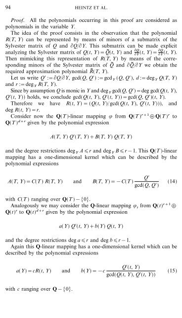
94 HEINTZ ET AL.
Proof. All the polynomials occurring in this proof are considered as
polynomials in the variable Y.
The idea of the proof consists in the observation that the polynomial
R(T, Y) can be represented by means of minors of a submatrix of the
Sylvester matrix of Q and QY. This submatrix can be made explicit
analyzing the Sylvester matrix of Q(t, Y)=Q (t, Y) and Q
Y
(t, Y)=Q
Y
(t, Y).
Then mimicking this representation of R(T, Y) by means of the corresponding
minors of the Sylvester matrix of Q and Q Y we obtain the
required approximation polynomial R (T, Y).
Let us write Q$:=QY, gcd(Q, Q$) :=gcd Y (Q, Q$), d :=deg Y Q(T, Y)
and r :=deg Y R(T, Y).
Since by assumption Q is monic in Y and deg Y gcd(Q, Q$)=deg gcd(Q(t, Y),
Q$(t, Y)) holds, we conclude gcd(Q(t, Y), Q$(t, Y))=gcd(Q, Q$)(t, Y).
Therefore we have R(t, Y)=(Q(t, Y)gcd(Q(t, Y), Q$(t, Y))), and
deg R(t, Y)=r.
Consider now the Q(T )-linear mapping . from Q(T ) r+1 Q(T ) r to
Q(T ) d+r given by the polynomial expression
A(T, Y) Q$(T, Y)+B(T, Y) Q(T, Y)
and the degree restrictions deg Y Ar and deg Y Br&1. This Q(T )-linear
mapping has a one-dimensional kernel which can be described by the
polynomial expressions
A(T, Y)=C(T ) R(T, Y) and B(T, Y)=&C(T )
Q$
gcd(Q, Q$)
(14)
with C(T ) ranging over Q(T )&[0].
Analogously we may consider the Q-linear mapping . t from Q(t) r+1
Q(t) r to Q(t) d+r given by the polynomial expression
a(Y) Q$(t, Y)+b(Y) Q(t, Y)
and the degree restrictions deg ar and deg br&1.
Again this Q-linear mapping has a one-dimensional kernel which can be
described by the polynomial expressions
a(Y)=cR(t, Y) and b(Y)=&c
Q$(t, Y)
gcd(Q(t, Y), Q$(t, Y))
(15)
with c ranging over Q&[0].