Deformation Techniques for Efficient Polynomial Equation ... - RISC

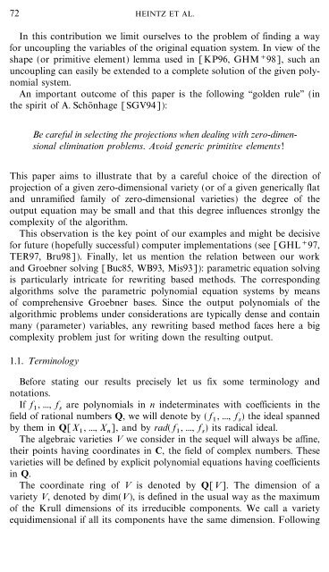
72 HEINTZ ET AL.
In this contribution we limit ourselves to the problem of finding a way
for uncoupling the variables of the original equation system. In view of the
shape (or primitive element) lemma used in [KP96, GHM + 98], such an
uncoupling can easily be extended to a complete solution of the given polynomial
system.
An important outcome of this paper is the following ``golden rule'' (in
the spirit of A. Scho nhage [SGV94]):
Be careful in selecting the projections when dealing with zero-dimensional
elimination problems. Avoid generic primitive elements!
This paper aims to illustrate that by a careful choice of the direction of
projection of a given zero-dimensional variety (or of a given generically flat
and unramified family of zero-dimensional varieties) the degree of the
output equation may be small and that this degree influences stronlgy the
complexity of the algorithm.
This observation is the key point of our examples and might be decisive
for future (hopefully successful) computer implementations (see [GHL + 97,
TER97, Bru98]). Finally, let us mention the relation between our work
and Groebner solving [Buc85, WB93, Mis93]): parametric equation solving
is particularly intricate for rewriting based methods. The corresponding
algorithms solve the parametric polynomial equation systems by means
of comprehensive Groebner bases. Since the output polynomials of the
algorithmic problems under considerations are typically dense and contain
many (parameter) variables, any rewriting based method faces here a big
complexity problem just for writing down the resulting output.
1.1. Terminology
Before stating our results precisely let us fix some terminology and
notations.
If f 1 , ..., f s are polynomials in n indeterminates with coefficients in the
field of rational numbers Q, we will denote by ( f 1 , ..., f s ) the ideal spanned
by them in Q[X 1 , ..., X n ], and by rad( f 1 , ..., f s ) its radical ideal.
The algebraic varieties V we consider in the sequel will always be affine,
their points having coordinates in C, the field of complex numbers. These
varieties will be defined by explicit polynomial equations having coefficients
in Q.
The coordinate ring of V is denoted by Q[V]. The dimension of a
variety V, denoted by dim(V), is defined in the usual way as the maximum
of the Krull dimensions of its irreducible components. We call a variety
equidimensional if all its components have the same dimension. Following