Lecture 10: From Analog to Digital Controllers A Digital Control ...
Lecture 10: From Analog to Digital Controllers A Digital Control ...
Lecture 10: From Analog to Digital Controllers A Digital Control ...

Create successful ePaper yourself
Turn your PDF publications into a flip-book with our unique Google optimized e-Paper software.
<strong>Lecture</strong> <strong>10</strong>:<br />
<strong>From</strong> <strong>Analog</strong> <strong>to</strong> <strong>Digital</strong> <strong><strong>Control</strong>lers</strong><br />
u( t )<br />
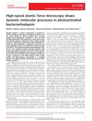
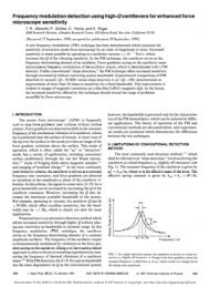
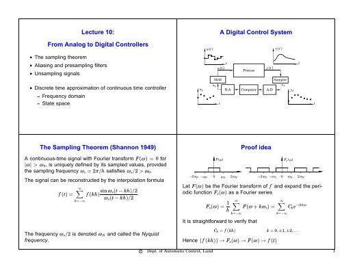
A <strong>Digital</strong> <strong>Control</strong> System<br />
y ( t )<br />
• The sampling theorem<br />
• Aliasing and presampling filters<br />
• Unsampling signals<br />
• Discrete time approximation of continuous time controller<br />
– Frequency domain<br />
– State space<br />
u k<br />
u( t )<br />
t<br />
Process<br />
Hold<br />
Sampler<br />
u k<br />
y k<br />
D-A Computer A-D y k<br />
t<br />
t<br />
y(<br />
t<br />
)<br />
t<br />
The Sampling Theorem (Shannon 1949)<br />
Proof idea<br />
A continuous-time signal with Fourier transform F(ω ) = 0 for<br />
|ω | > ω 0 , is uniquely defined by its sampled values, provided<br />
the sampling frequency ω s = 2π /h satisfies ω s /2 > ω 0 .<br />
The signal can be reconstructed by the interpolation formula<br />
f (t) =<br />
∞∑<br />
k=−∞<br />
f (kh) sinω s(t − kh)/2<br />
ω s (t − kh)/2<br />
−2ω N<br />
−ωN<br />
0<br />
F(ω)<br />
ω N<br />
2ω N<br />
F s (ω)<br />
−2ω N −ω N 0 ω N 2ω N<br />
Let F(ω ) be the Fourier transform of f and expand the periodic<br />
function F s (ω ) as a Fourier series<br />
F s (ω ) = 1 h<br />
∞∑<br />
k=−∞<br />
F(ω + kω s ) =<br />
∞∑<br />
k=−∞<br />
C k e −ikhω<br />
It is straightforward <strong>to</strong> verify that<br />
The frequency ω s /2 is denoted ω N and called the Nyquist<br />
frequency.<br />
C k = f (kh) k = 0, ±1, ±2, . . .<br />
Hence {f (kh)} → F s (ω ) → F(ω ) → f (t)<br />
c Dept. of Au<strong>to</strong>matic <strong>Control</strong>, Lund 1
¡<br />
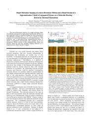
Aliasing and frequency folding<br />
1<br />
Aliasing and presampling filters<br />
0<br />
0 5 <strong>10</strong><br />
Time<br />
F (ω ) F s (ω )<br />
−2ω N<br />
−ωN<br />
0<br />
ω N<br />
2ω N<br />
−2ω N −ω N 0 ω N 2ω N<br />
ω N = ω s /2 Nyquist frequency<br />
New frequencies since the system is NOT time-invariant<br />
ω sampled = ω + nω s n = 0, ±1, ±2, . . .<br />
Mini-problem<br />
Example — Feedwater heating in a ship boiler<br />
A wheel, rotating 90 turns per second, is filmed using a<br />
camera with sampling time <strong>10</strong>ms. What will the wheel rotation<br />
look like on the film?<br />
Feed<br />
water<br />
Pressure<br />
Pump<br />
Steam<br />
Valve<br />
To boiler<br />
Temperature<br />
38 min<br />
2 min<br />
Condensed<br />
water<br />
Temperature<br />
Pressure<br />
2.11 min<br />
Time<br />
c Dept. of Au<strong>to</strong>matic <strong>Control</strong>, Lund 2
¡<br />
¡<br />
¡<br />
¡<br />
¥<br />
¢<br />
§¦<br />
¥<br />
¢<br />
¤£<br />
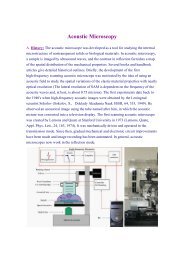
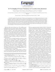
Pre- and postsampling filters<br />
Example – Prefiltering<br />
Typical control problem:<br />
(a)<br />
1<br />
(b)<br />
1<br />
"Decrease the influence of a low-frequency process disturbance<br />
despite high-frequency measurement noise."<br />
0<br />
0<br />
• Frequency separation<br />
• Prefilter ω N<br />
– Bessel, Butterworth, ITAE filters<br />
(c)<br />
0 <strong>10</strong> 20 30<br />
1<br />
(d)<br />
0 <strong>10</strong> 20 30<br />
1<br />
• Postsampling filters<br />
0<br />
0<br />
– Avoid exciting mechanical resonances<br />
– Higher order hold<br />
0 <strong>10</strong> 20 30<br />
Time<br />
0 <strong>10</strong> 20 30<br />
Time<br />
ω d = 0.9, ω N = 0.5, ω alias = 0.1 (6th order Bessel filter)<br />
Consequence of using prefilter<br />
Pre- and postfilter should be included in the process model<br />
Exception: Fast sampling<br />
A Besselfilter can be approximated with a delay:<br />
• Shannon<br />
Unsampling signals<br />
f (t) =<br />
∞∑<br />
k=−∞<br />
f (kh) sin(ω s(t − kh)/2)<br />
ω s (t − kh)/2<br />
Gain<br />
1<br />
0.01<br />
0.1 1 <strong>10</strong><br />
0<br />
• Zero order hold<br />
• First order hold<br />
Phase<br />
• Predictive first order hold<br />
0.1 1 <strong>10</strong><br />
Frequency, rad/s<br />
6th order Bessel (solid line), time delay (dashed line)<br />
c Dept. of Au<strong>to</strong>matic <strong>Control</strong>, Lund 3
¢¡<br />
¤<br />
£<br />
¤<br />
£<br />
¤<br />
£<br />
¤<br />
£<br />
¤<br />
£<br />
¤<br />
£<br />
Shannon reconstruction<br />
f (t) =<br />
∞∑<br />
k=−∞<br />
The exact formula is not causal !<br />
f (kh) sin(ω s(t − kh)/2)<br />
ω s (t − kh)/2<br />
Approximation with information from d time steps ahead:<br />
ˆ f (nh + τ ) =<br />
∑n+d<br />
k=−∞<br />
f (kh)h(nh + τ − kh) h(τ ) = sinω sτ /2<br />
ω s τ /2<br />
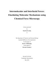
Zero and first order hold<br />
t 0 t 1 t 2 t 3 t 4 t 5<br />
t 6 Time<br />
1<br />
0<br />
sinπ t<br />
π t<br />
0 <strong>10</strong><br />
Time<br />
t 0 t 1 t 2 t 3 t 4 t 5<br />
t 6 Time<br />
Predictive first order hold<br />
Sinusoidal signal with h = 1 and h = 0.5<br />
• Use forward difference instead of backward difference<br />
u(kh + τ ) = u(kh) + τ (u(kh + h) − u(kh))<br />
h<br />
• Use model of the controller.<br />
Zero order hold<br />
h=1<br />
1<br />
0<br />
0 5 <strong>10</strong><br />
Zero order hold<br />
h=0.5<br />
1<br />
0<br />
0 5 <strong>10</strong><br />
First order hold<br />
1<br />
0<br />
First order hold<br />
1<br />
0<br />
0 5 <strong>10</strong><br />
0 5 <strong>10</strong><br />
t 0 t 1<br />
t 2 t 3<br />
t 4<br />
t 5<br />
t 6 Time<br />
Predictive hold<br />
1<br />
0<br />
Predictive hold<br />
1<br />
0<br />
0 5 <strong>10</strong><br />
Time<br />
0 5 <strong>10</strong><br />
Time<br />
c Dept. of Au<strong>to</strong>matic <strong>Control</strong>, Lund 4
Implementing a controller using a computer<br />
H(z) ≈ G (s)<br />
Discrete time approximation of<br />
continuous time controller<br />
— Frequency domain<br />
u(t)<br />
Want <strong>to</strong> get<br />
Methods:<br />
A-D<br />
{ u( kh )} { y( kh )}<br />
Algorithm<br />
Clock<br />
D-A<br />
A/D + Algorithm + D/A ≈ G(s)<br />
• Approximate s i.e G(s) → H(z)<br />
• Pole-zero matching<br />
• Use sample/hold <strong>to</strong> get H(z) from G(s)<br />
y(t)<br />
Matlab<br />
SYSD = C2D(SYSC,TS,METHOD) converts the continuous<br />
system SYSC <strong>to</strong> a discrete-time system SYSD with<br />
sample time TS. The string METHOD selects the<br />
discretization method among the following:<br />
’zoh’ Zero-order hold on the inputs.<br />
’foh’ Linear interpolation of inputs<br />
(triangle appx.)<br />
’tustin’ Bilinear (Tustin) approximation.<br />
’prewarp’ Tustin approximation with frequency<br />
prewarping.<br />
The critical frequency Wc is specified<br />
last as in C2D(SysC,Ts,’prewarp’,Wc)<br />
’matched’ Matched pole-zero method<br />
(for SISO systems only).<br />
Approximation methods<br />
Forward difference (Euler’s method)<br />
dx(t)<br />
dt<br />
Backward difference<br />
dx(t)<br />
dt<br />
≈<br />
≈<br />
x(t + h) − x(t)<br />
h<br />
x(t) − x(t − h)<br />
h<br />
Trapezoidal method (Tustin, bilinear)<br />
ẋ(t + h) + ẋ(t)<br />
2<br />
≈<br />
= q − 1<br />
h<br />
= 1 − q−1<br />
h<br />
x(t + h) − x(t)<br />
h<br />
x(t)<br />
x(t)<br />
c Dept. of Au<strong>to</strong>matic <strong>Control</strong>, Lund 5
Mini-problem<br />
Compare the differential equation<br />
ẏ(t) + <strong>10</strong>y(t) = 0<br />
<strong>to</strong> the Euler approximation<br />
y(k + 1) − y(k) + <strong>10</strong>y(k) = 0<br />
Is there any qualitative difference?<br />
What is the source of the problem?<br />
Properties of the approximation H(z) ≈ G(s)<br />
s = z − 1<br />
h<br />
s = z − 1<br />
s = 2 h<br />
zh<br />
z − 1<br />
z + 1<br />
(Forward difference or Euler’s method)<br />
(Backward difference)<br />
(Tustin’s or bilinear approximation)<br />
Where do stable poles of G get mapped?<br />
Forward differences Backward differences Tustin<br />
Prewarping <strong>to</strong> reduce frequency dis<strong>to</strong>rtion<br />
s<br />
iω ′<br />
−iω ′<br />
Choose one fix-point ω 1<br />
s =<br />
z<br />
e iω ′<br />
ω 1<br />
tan(ω 1 h/2) ⋅ z − 1<br />
z + 1<br />
e −iω ′<br />
Approximation<br />
Pole-zero matching<br />
1. All poles of G(s) are mapped according <strong>to</strong> z = e sh<br />
2. All finite zeros are also mapped as z = e sh<br />
3. The zeros of G(s) at s = ∞ are mapped in<strong>to</strong> z = −1. One<br />
of the zeros of G(s) at s = ∞ is mapped in<strong>to</strong> z = ∞, i.e.<br />
deg A(z) − deg B(z) = 1<br />
4. The gain of H(z) is matched the gain of G(s) at one<br />
frequency, center frequency or at steady-state, s = 0<br />
This implies that H ( e ) iω 1h<br />
= G(iω 1 ) Tustin is obtained for<br />
ω 1 = 0 since tan ( )<br />
ω 1 h<br />
2 ≈<br />
ω 1 h<br />
for small ω .<br />
2<br />
c Dept. of Au<strong>to</strong>matic <strong>Control</strong>, Lund 6
£ §<br />
£ ¦<br />
£ ¥<br />
£ ¤<br />
¢¡<br />
¢<br />
¨ 0©<br />
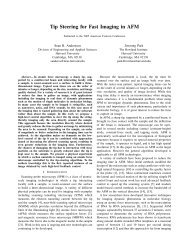
Comparison of approximations<br />
(s + 1) 2 (s 2 + 2s + 400)<br />
G(s) =<br />
(s + 5) 2 (s 2 + 2s + <strong>10</strong>0)(s 2 + 3s + 2500)<br />
h = 0.03 gives ω N = <strong>10</strong>5 rad/s<br />
Magnitude<br />
<strong>10</strong><br />
<strong>10</strong><br />
<strong>10</strong><br />
<strong>10</strong><br />
<strong>10</strong> 0 <strong>10</strong> 1 <strong>10</strong> 2<br />
Selection of sampling interval<br />
The Zero-Order-Hold has the transfer function<br />
For small h<br />
1 − e −sh<br />
sh<br />
G ZoH (s) = 1 − e−sh<br />
sh<br />
≈ 1 − 1 + sh − (sh)2 /2 + ⋅ ⋅ ⋅<br />
sh<br />
exp(−sh/2) ≈ 1 − sh 2 + ⋅ ⋅ ⋅<br />
= 1 − sh 2 + ⋅ ⋅ ⋅<br />
Phase<br />
0<br />
<strong>10</strong> 0 <strong>10</strong> 1 <strong>10</strong> 2<br />
Frequency, rad/s<br />
G ZoH (s) can be approximated as a delay h/2<br />
Assume the phase margin can be decreased by 5 ○ <strong>to</strong> 15 ○ then<br />
hω c ≈ 0.15 − 0.5<br />
G(iω ) (full), zoh (dashed), foh (dot-dashed), Tustin (dotted)<br />
This leads <strong>to</strong> ω N 5–20 larger than ω c<br />
<strong>Digital</strong> redesign of lead compensa<strong>to</strong>r<br />
A lead compensa<strong>to</strong>r G(s) = 4(s + 1)/(s + 2) for the process<br />
P(s) = 1/(s 2 + s) gives ω c = 1.6. Hence choose h = 0.1 − −0.3.<br />
Euler’s method: H E (z) = 4<br />
Output<br />
1<br />
z−1<br />
h + 1 z − (1 − h)<br />
= 4<br />
+ 2 z − (1 − 2h)<br />
z−1<br />
h<br />
Discrete time approximation of<br />
continuous time controller<br />
— State space<br />
0<br />
0 <strong>10</strong><br />
4<br />
Input<br />
2<br />
0 <strong>10</strong><br />
Time<br />
h = 0.1 (dash-dotted), 0.25 (full), 0.5 (dotted), G(iω ) (dashed)<br />
c Dept. of Au<strong>to</strong>matic <strong>Control</strong>, Lund 7
¤<br />
¡£¢<br />
¤<br />
¡£¢<br />
¥<br />
¥<br />
State-feedback redesign<br />
The system ẋ = Ax + Bu with continuous-time state feedback<br />
u(t) = Mu c (t) − Lx(t)<br />
gives ẋ = (A − B L) x + BMu<br />
} {{ }<br />
c = A c x + BMu c Sampling gives<br />
A c<br />
x(kh + h) = Φ c x(kh) + Γ c Mu c (kh)<br />
Alternatively, sampling first, then applying discrete-time state<br />
feedback<br />
u(kh) = ˜Mu c (kh) − ˜Lx(kh)<br />
gives<br />
x(kh + h) = (Φ − Γ ˜L)x(kh) + Γ ˜Mu c (kh)<br />
State feedback redesign cont’d<br />
With ˜L = L 0 + L 1 h/2 the two system matrices<br />
Φ c = I + (A − B L)h + ( A 2 − B LA − AB L + (B L) 2) h 2 /2 + ⋅ ⋅ ⋅<br />
Φ − Γ ˜L = I + (A − B L 0 )h + ( A 2 − AB L 0 − B L 1<br />
) h 2 /2 + ⋅ ⋅ ⋅<br />
are identical of order h 2 provided that L 0 = L, L 1 = A − B L.<br />
To make the steady-state gain correct, let ˜M = M 0 + M 1 h/2<br />
and compare<br />
Γ c M = B M h + (A − B L)B M h 2 /2 + ⋅ ⋅ ⋅<br />
Γ ˜M = B M 0 h + (B M 1 + AB M 0 )h 2 /2 + ⋅ ⋅ ⋅<br />
The expressions are identical of order h 2 provided that<br />
M 0 = M, M 1 = −LBM.<br />
State-feedback redesign – Example<br />
Double integra<strong>to</strong>r with h = 0.5, L = [1 1], and M = 1<br />
Position<br />
1<br />
Position<br />
1<br />
0<br />
0 <strong>10</strong><br />
0<br />
0 <strong>10</strong><br />
Velocity<br />
0.5<br />
0<br />
Velocity<br />
0.5<br />
0<br />
0 <strong>10</strong><br />
0 <strong>10</strong><br />
1<br />
1<br />
Input<br />
0<br />
Input<br />
0<br />
0 <strong>10</strong><br />
Time<br />
0 <strong>10</strong><br />
Time<br />
˜L =<br />
⎧<br />
⎩ 1 − 0.5h 1<br />
⎫<br />
⎭ ˜M = 1 − 0.5h<br />
c Dept. of Au<strong>to</strong>matic <strong>Control</strong>, Lund 8